Trading leads to scale-free self-organization

Abstract

Financial markets display scale-free behavior in many different aspects. The power-law behavior of part of the distribution of individual wealth has been recognized by Pareto as early as the nineteenth century. Heavy-tailed and scale-free behavior of the distribution of returns of different financial assets have been confirmed in a series of works. The existence of a Pareto-like distribution of the wealth of market participants has been connected with the scale-free distribution of trading volumes and price-returns. The origin of the Pareto-like wealth distribution, however, remained obscure. Here we show that it is the process of trading itself that under two mild assumptions spontaneously leads to a self-organization of the market with a Pareto-like wealth distribution for the market participants and at the same time to a scale-free behavior of return fluctuations. These assumptions are (i) everybody trades proportional to his current capacity and (ii) supply and demand determine the relative value of the goods.

Exchange of goods, i.e. trading, is a process as old as humanity. We show here that under two rather mild assumptions trading always leads to a Pareto-type wealth distributionpareto and the non-Gaussian price fluctuations mandelbrot ; ms-nature-95 ; stanley-new that have attracted the interest of statistical physicists stanley ; bouchaud . Price fluctuations of financial assets display heavy-tailed non-Gaussian behavior over a broad range of time scales before becoming Gaussian as required by the central limit theorem. Their distribution has been described by truncated Lévy distributionstr-levy as well as having a power-law tail with an exponent around $x=-4$ outside the range of Lévy-like power law tails stan-powerlaw . Both descriptions, however, contain scale-invariant power-law distributions of the price fluctuations over a limited range in size and over a limited time horizon. Another well-known and famous power-law occurring in our societies is the Pareto law of wealth distributionpareto . This law has not only been found for the wealth of individuals unu but also for the size of companies wealth-comp .

We will show that the simplest imaginable model of trading, where trading decisions are made randomly, where always a finite fraction of available goods is invested and where the imbalance between supply and demand changes the price of goods, is sufficient to produce a Pareto type wealth distribution as well as scale-free fluctuations of the market. In fact, independent of the choice of parameters, our model market always self-organizes into a stationary, scale-free state. Only the duration of the transient, and parameters quantifying the transient and the stationary state are influenced by the choice of the model parameters.

Agent based models are commonly used to analyze markets. But often the complexity of these models obscures the cause of the observed market behavior. We are therefore looking at a minimal model for agent based trading. Our model simulates the exchange of two goods. We will call them stock and money from here on but this denomination is arbitrary and only serves to facilitate the description of the results. Each agent at each time step randomly decides whether he wants to buy or sell stock. The quantity of money spent on buying stock, or stock sold for money is also determined randomly, varying between nothing and an investment fraction $c$ of the agents current posession in stock or money, respectively.

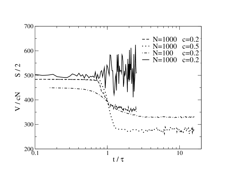
Figure 1: Trading volume per time step normalized to its expected average value $1000Nc/2$ for several choices of numer of agents $N$ and investment fraction $c$ (broken curves) and price development for one of these cases (full curve) as a function of scaled time. The time scaling $\tau$ is chosen as the center of the crossover from high trading volume to low trading volume.

Agents are not allowed to leave or enter the market and neither stock nor money may be created or destroyed. The price is determined by supply $S$ and demand $D$. To capture the conviction that supply and demand determine the price one could use a simple ansatz to adjust the price $p$ in each time step according to $p(n+1)=p(n)D/S$. To avoid the singularity for $S=0$ we instead used

$$p(n+1)=p(n)[1+(D-S)/(D+2S)]=p(n)[1+f(S,D)]$$ (1)

This formula limits price fluctuations in each time step to a factor of $2$, is differentiable and has no singularities. Several possibilities for price changes have been analyzed, however, and we found that our model is not sensitive to the choice of price update function, as long as it guarantees a price adjustment monotonously depending on the imbalance between supply and demand. We can write down the master equation for the probability $P(A,G,n+1)$ for an agent to possess a number $A$ of stocks and an amount $G$ in money at time step $n+1$:

$$P\left(A,G,n+1\right)=(1-q(n))P\left(A,G,n\right)$$ (2)

$$+\frac{q(n)}{2c}\sum_{A^{\prime}=A-\frac{cG^{\prime}}{p(n)}}^{A-1}\frac{P\left(A^{\prime},G+(A^{\prime}-A)p(n),n\right)}{G+(A^{\prime}-A)p(n)}$$

$$+\frac{q(n)}{2c}\sum_{A^{\prime}=A+1}^{A/(1-c)}\frac{P\left(A^{\prime},G+(A^{\prime}-A)p(n),n\right)}{A^{\prime}}$$

with

$$q(n)=1-\left|\frac{\sum_{i}x_{i}(n)\left(A_{i}(n)-\frac{G_{i}(n)}{p(n)}\right)}{\sum_{j}x_{j}(n)\left(A_{j}(n)+\frac{G_{j}(n)}{p(n)}\right)}\right|$$ (3)

being the propability of a trade attempt actually happening. $x_{i}(n)$ is the fraction of stock or money of agent $i$ traded in the step, randomly chosen between $0$ and $c$. We begin our simulations in a perfect socialistic state: all agents possess the same wealth, e.g. $1000$ stocks worth $1000$ units and $1000000$ units of money. The time evolution of trading volume and stock price generated by our market model are shown in Fig. 1. For several choices of the number of participating agents $N$ and investment fraction $c$, Fig. 1 shows that there is a crossover between two dynamic regimes. Between the two regimes the trading volume decreases and simultaneously the average price increases and also the price fluctuations increase at a crossover time $\tau$ that scales as $(N/c)2$ (Fig. 1 displays this crossover in scaled time).

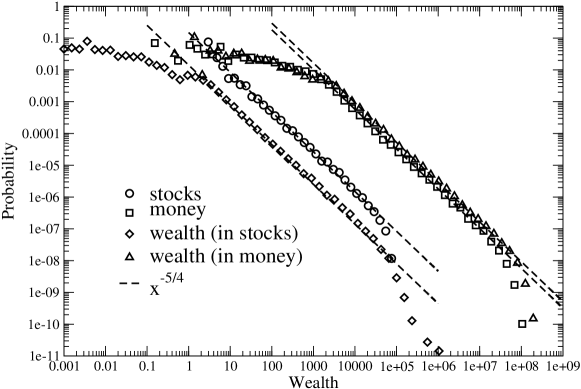
Figure 2: Probability density for stocks owned (circles), money owned (squares), total wealth measured in stocks (diamonds) and total wealth measured in money (triangles) for $N=200$ agents and investment fraction $c=0.5$.

The initial regime is characterized by Gaussian fluctations. The initial $\delta$-distribution of wealth spreads into a Gaussian distribution with increasing width. When the influence of the boundary at zero wealth starts to be felt, the wealth distribution changes into a lognormal form with a center which moves towards zero wealth. If growth of wealth would be strictly proportional to existing wealth gibrat this would be a stationary state of the wealth distribution. Furthermore, in this early time regime the price fluctuates around an equilibrium value which is simply given by the available money per stock. If one does not start the simulation with this value, the price adjusts to it within a few time steps. Price fluctuations are Gaussian and the distribution of trading volumes in one time step is Gaussian as well.

However, this regime is not dynamically stable. The wealth distribution develops heavy tails and finally crosses over to its stationary shape which displays power law behavior. This is shown in Fig. 2 which shows several measures of the wealth per agent in the stationary state for a system with $N=200$ agents which invest at most $50$ % of their wealth in each step. In the stationary regime, the distribution of stocks per agent is a perfect power law with an exponent $x=-1.25$, i.e., the trading process leads to a self-organization of the market into a scale-free state. Varying the number of agents between $N=100$ and $N=1000$ and the investment fraction between $c=0.2$ and $c=0.9$ we always find a power law behavior with exponent around $x\simeq-1.3$. The distribution of money owned is almost constant for small amounts of money, then crosses over to the same power law found for the number of stocks owned and finally, for large amounts of money, a steeper decay is found which reflects the finiteness of the money present in the market. To determine the total wealth of an individual, we can either express wealth in units of stocks or express it in units of money. The money value of an amount of $A(n)$ stocks is $G(n)=p(n)A(n)$, and the stock value of an amount of money $G(n)$ is $A(n)=G(n)/p(n)$, where $p(n)$ is the current price of stocks on the market. Thus total wealth always depends on the price dynamics and this enters asymmetrically between stocks and money. However, for the case of $c=0.5$ shown in the Fig. 2 both ways of measuring wealth show power law regimes over $3-4$ orders of magnitude with the same epxonent of $x=-1.25$ as the other distributions. The price fluctations only shift the wealth distribution expressed in money to slightly larger wealth values. This is changed for large $c$ where both distributions show a differing power law exponent due to the qualitative change in price fluctuations observed then (see Fig. 4). Although the exponent found for the scale invariant part of the wealth distribution differs from the typical value $x_{P}\simeq 2.5$ found for example for a recent study on the world distribution of household wealth unu , our very simplified economy is able to capture the emergence of a Pareto law. It is also interesting to note, that in the scale-free state, the average stock price is larger than the average money available per stock.

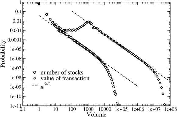
Figure 3: Probability density for the trading volume per transaction and money invested per ransaction for an investment fraction of $c=0.5$.

There have been several attempts in recent years to explain the origins of the Pareto distribution of wealth by assuming interactions between agents to resemble collisions between particles, as treated using kinetic theory in statistical physics. Often, the exchange of wealth in these binary collisions is modelled by a multiplicative stochastic process solomon . If $W_{i}(n)$ is the wealth of agent $i$ at time $n$, one writes $W_{i}(n+1)=W_{i}(n)(1+\epsilon\xi(n))$ where $\epsilon<<1$ is a small amplitude and $\xi(n)$ a random number in $[0,1)$. The stationary distribution of wealth is then scale-free, generally with an exponent $x=-2$ chak-2003 , also not in agreement with the empirical value $x_{P}$. Introduction of heterogeneous behavior among the agents, e.g., in the form of a random saving propensity chak-2007 ; germ-2006 can change the observed exponent to the empirical value. The generic behavior of these kinetic models for wealth redistribution has also been worked out duering ; lammoglia .

In contrast to this approach, in our model wealth changes in a trade only due to the update of the price of goods. The wealth change of an agent is asymmetric between buyers and sellers

$$W_{i}(n+1) = W_{i}(n)[1+f(S,D)(1-c\xi(n))]$$

$$- f(S,D)(1-\xi(n))G_{i}(n)\quad\mbox{(seller)}$$

$$W_{i}(n+1) = W_{i}(n)[1+f(S,D)c\xi(n)]$$

$$- f(S,D)(1-\xi(n))A_{i}(n)p(n)\quad\mbox{(buyer)}$$

where $\xi(n)$ is a uniform random number in $[0,1)$. The trading process itself (i.e., the collision between the particles in the physical analogy) does not change the wealth of the agents, as they only exchange stocks for money and vice versa. Only the interaction between trading process and price update leads to a change of wealth and the observed self-organization of the wealth distribution into a Pareto-like state. For this to occur one has to have at least two goods which are traded, one of which is conveniently identified as money. This simplest possible economy thus inevitably leads to a Pareto-like behavior for large wealths.

We argued that it is the coupling of trading to the price process that leads to the observed power-law behavior. So let us now look at the stationary behavior for the price fluctuations. Gabaix et al. stanley-nature-2003 presented a model which linked the presence of a Pareto-type distribution of the wealth of market participants to the occurrence of power law tails in the distribution of trading volumes and price fluctuations. The exponents characterizing these power laws $p(|r_{t}|>z)\propto z^{-\beta}$ and $p(V_{t}>u)\propto u^{-\gamma}$ where $r_{t}=ln[p(t_{0}+t)/p(t)]$ is the return on a time horizon $t$ and $V_{t}$ is the volume traded on time horizon $t$, are related through the price impact function. Several empirical studies of different markets citevolume-impact,farmer,zhou have established that over a reasonable range in volumes, price impact and volume are related through a power law dependence $\Delta p\propto V^{\alpha}$. From this it follows that $\beta=\alpha\gamma$. The observed exponents are $\alpha\simeq 1/2$ volume-impact ; farmer , $\alpha\simeq 0.2$ for larger volumes farmer and $\alpha\simeq 0.6-0.7$ zhou .

The distribution of volumes for individual trades in our model is shown in Fig. 3. Both in terms of number of stocks traded and in terms of money value of the transaction the volume obeys a power law scaling with the same exponent as the wealth distribution (i.e. $\alpha=1$) over three orders of magnitude before the cutoff due to finite total wealth in the system sets in. For small volumes there seems to exist another regime which is dominated by the low-end part of the wealth distribution. Our model therefore conforms to the phenomenological finding that a power law wealth distribution gives rise to a power law volume distribution. The price, however, is updated according to the difference between supply and demand as given by equ.( 1). The update function depends on the imbalance between supply and demand, $I=S-D$, and the cumulative volume $V=min(S,D)$ of all trades in one Monte Carlo step This distribution does not show a scale-free regime, displays a maximum at intermediate volumes and can be phenomenologically described by a lognormal form. The distribution broadens with increasing investment fraction and becomes highly assymmetric for large investment fraction. For all choices of investment fraction this leads to non-Gaussian heavy tails in the distribution of price fluctuations as shown in Fig. 4. The Lévy-tails found for $c=0.9$ are the origin of the different behavior of the wealth distribution whether expressed in number of stocks or in money (discussed for Fig. 2), since the latter is susceptible to the Lévy-type fluctuations in the price. For an intermediate range of investment fractions, however, the tail of the distribution of price flucuations is compatible with the behavior phenomenologically found for real markets. For $c=0.5$ we even recover the exponent $x=-4$ found in Ref. stan-powerlaw .

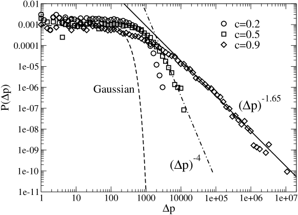
Figure 4: Probability density for price fluctions in one Monte Carlo step. For all choices of investment fraction c we obtain distributions with a fat tail compared to the Gaussian behavior. For small and intermediate c the tail behavior is compatible with the market phenomenology, for $c=0.9$ we obtain a Lévy-type fat tail.

The market behavior discussed above remains qualitatively unchanged when we include interest in our model (i.e., increase the money available to the agents by a fixed rate), the price however, now fluctuates around an increasing average. We would like to note also that our model remains strictly egalitarian. There is no symmetry breaking between the different agents and each agent wanders up and down the wealth curve in the course of the simulation (which is, of course, not very realistic). This shortcoming and the deviation of the Pareto exponent from the phenomenologically observed one can be amendet when one introduces heterogeneous trading strategies among the agents. One could even solve an inverse problem to determine the trading strategy leading to the correct exponent lammoglia . However, we would like to emphasize here that already the extremely simplified model we introduced captures the emergence of the Pareto law and the qualitative relations between wealth distribution and market fluctuations.

The self-organization of the market into a scale-free wealth state and the connection between the wealth distribution and the price fluctuations found at the market lends itself to a consideration of the effect that leverage has in such a situation. The importance of leverage to generate the Pareto-tail of the wealth distribution has been discussed long ago by Montroll and Shlesinger montroll . Leverage virtually increases the amount of money present in the system and with that the point to which the Pareto-like wealth distribution extends before it is cut off. The extend of the Pareto distribution in turn, determines the scale of the price fluctuations, Employing leverage thus increases the scale of the fluctuations present in the market. When too much leverage is employed this creates downward-fluctuations exceeding the real existing wealth of the agents, arguably leading to the credit defaults the financial markets are plagued with at the moment. Our simple model also suggests that economic inequality gibrat is almost as old as humankind. When the first trading good was invented that could be used in the way money is used today, and was not meant to be directly consumed or used up in other ways in daily life, fluctuations in the exchange rate of this good with others destabilized the state of economic equality and led to a Pareto-type wealth distribution.

Acknowledgement: The authors thank J. J. Schneider, T. Preis and J. Zausch for discussions.

References

- (1) Pareto, V. Cours d’Economique Politique (F. Rouge, Lausanne, 1897).
- (2) B. B. Mandelbrot, J. Business 36, 394 (1963).
- (3) R. N. Mantegna and H. E. Stanley, Nature 376, 46 (1995).
- (4) V. Plerou and H. E. Stanley, Phys. Rev. E 77, 037101 (2008).
- (5) R. N. Mantegna and H. E. Stanley, Introduction to Econophysics: Correlations & Complexity in Finance (Cambridge University Press, Cambridge, 2000).
- (6) J.-P. Bouchaud and M. Potters, Theory of Financial Risks, (Cambridge University Press, 2000).
- (7) R. N. Mantegna and H. E. Stanley, Phys. Rev. Lett. 73, 2946 (1994).
- (8) P. Gopikrishnan et al. Phys. Rev. E 60, 5305 (1999).
- (9) J. B. Davies, S. Sandstrom, A. Shorrocks and E. N. Wolff, The World Distribution of Household Wealth (UNU-WIDER, Helsinki,2006), http://www.wider.unu.edu
- (10) R. Axtell, Science 293, 1818 (2001).
- (11) R. Gibrat, Lés Inégalités Economique (Sirey, Paris, 1933).
- (12) H. Levy, S. Solomon and M. Levy, Microscopic Simulation of Financial Markets: From Investor Behavior to Market Phenomena (Academic Press, 2000).
- (13) A. Chatterjee, B. K. Chakrabarti and R. B. Stinchcombe, Phys. Rev. E 72, 026126 (2005).
- (14) A. Chatterjee and B. K. Chakrabarti, Eur. Phys. J. B 60, 135 (2007).
- (15) M. Patriarca, A. Chakraborti, a nd G. Germano, Physica 369, 723 (2006).
- (16) B. Düring, D. Matthes and G. Toscani, Phys. Rev. E 78, 056103 (2008).
- (17) N. Lammoglia et al. Phys. Rev. E 78, 047103 (2008).
- (18) X. Gabaix, P. Gopikrishnan, V. Plerou and H. E. Stanley, Nature 423, 267 (2003).
- (19) V. Plerou, P. Gopikrishnan, X. Gabaix, and H. E. Stanley, Phys. Rev. E 66, 027104 (2002).
- (20) F. Lillo, D. Farmer and R. N. Mantegna, Nature 421, 1290 (2003).
- (21) W. X. Zhou, Universal price impact functions of individual trades in an order-driven market, arXiv:0708.3198v2
- (22) E. W. Montroll and M. F. Shlesinger, On the Wonderful Word of Random Walks. in Nonequilibrium. Phenomena II, From Stochastics to Hydrodynamics. Lebowitz, L. & Montroll, E.W. eds. (North-Holland, Amsterdam, 1984).