Is spin-charge separation observable in a transport experiment?

Abstract

We consider a one-dimensional chain consisting of an interacting area coupled to non-interacting leads. Within the area, interaction is mediated by a local on-site repulsion. Using real time evolution within the Density Matrix Renormalisation Group (DMRG) scheme, we study the dynamics of wave packets in this two-terminal transport setup. In contrast to previous works, where excitations were created by adding potentials to the Hamiltonian, we explicitly create left moving single particle excitations in the right lead as the starting condition. Our simulations show that such a transport setup allows for a clear detection of spin-charge separation using time-resolved spin-polarised density measurements.

Introduction

Although spin-charge separation (SCS) is undisputed to happen in one-dimensional systems, its direct experimental observation and verification is a subject of many works over the past years. In one dimension, the Fermi liquid picture of non-interacting quasi-fermions is not appropriate Voit_RPP1995 . Instead, in the paradigmatic Tomonaga-Luttinger model and in the prototypical Hubbard model collective bosonic spin and charge excitations are the low-energy excitations. These so-called spinons carry spin but no charge and so-called holons carry the charge but no spin and spinons and holons may propagate with independent velocities.

Up to now few experimental setups barely show direct evidence of separate spin and charge excitations Halperin_JAP2007 . Beside tunnelling experiments e.g. momentum-conserved tunnelling on cleaved-edge overgrown GaAs/AlGaAs heterostructures Auslaender_Steinberg_Yacoby_Tserkovnyak_Halperin_Baldwin_Pfeiffer_West_S2005 and single-point tunnelling into carbon nanotubes Tombros_vanderMolen_vanWees_PRB2006 ; Bockrath_Cobden_Lu_Rinzler_Smalley_Balents_McEuen_N1999 , there is angle-resolved photo emission spectroscopy (ARPES) on quasi-one-dimensional SrCuO₂ material Kim_Koh_Rotenberg_Oh_Eisaki_Motoyama_Uchida_Tohyama_Maekawa_Shen_Kim_NPhys2006 and on the organic conductor TTF-TCNQ Claessen_Sing_Schwingenschlogl_Blaha_Dressel_Jacobsen_PRL2002 ; Sing_Schwingenschlogl_Claessen_Blaha_Carmelo_Martelo_Sacramento_Dressel_Jacobsen_PRB2003 which seem to show distinct spinon and holon branches in the spectral function. Numerical simulations explaining the latter experiments were done by Benthien et. al. Benthien_Gebhard_Jeckelmann_PRL2004 .

Here, we propose the following transport experiment: A one-dimensional interacting region is connected to non-interacting leads on both sides. In one of the leads a single electron with average momentum $k_{0}$ is injected into the system. The excitation, by passing through the interacting region, ends up in the other non-interacting lead, where a spin-resolved and time-resolved measurement of charge density is carried out. This setup poses the following questions which we answer in this paper: If one injects an electron with definite momentum at some time $t_{0}$ into an interacting system, where the separation of spin and charge is known to happen, what happens to the electronic excitation within the interacting region? And what kind of excitation emerges from the interacting area at a later time? Will we see distinct excitations in spin and charge density, will we find spin and charge density to be recombined to one full electronic excitation, or will we obtain an incoherent superposition of many excitations?

Safi and Schulz Safi_Schulz_PRB1999 analyse such a transport setup analytically for a spinless Tomonaga-Luttinger liquid model. For the spinful case, however, they have to neglect “umklapp processes and the backscattering of electrons with opposite spin” to sketch a qualitative picture, thus looking at an idealised system, where spin and charge currents are conserved separately. The first numerical simulations for spin-charge separation were performed by Jagla et. al. Jagla_Hallberg_Balseiro_PRB1993 using exact diagonalisation for 16 sites. Zacher et. al. Zacher_Arrigoni_Hanke_Schrieffer_PRB1998 used Quantum Monte Carlo simulations to study the spin and charge susceptibilities of the Hubbard model. Kollath et. al. Kollath_Schollwock_Zwerger_PRL2005 presented the first spin-charge separation calculations in the framework of adaptive time dependent DMRG (td-DMRG). This calculation was redone by Schmitteckert Schmitteckert_HPC2007 , keeping up to 5000 states per DMRG block showing that the adaptive time evolution scheme is prone to large numerical errors in the long time limit. In the same line, Schmitteckert and Schneider Schmitteckert_Schneider_HPC2006 used over 10000 states per DMRG block to show SCS in a 33 site system with periodic boundary conditions which avoids Friedel oscillations.

In order to avoid the numerical problem associated with the adaptive time evolution scheme and to avoid the numerical costs of a pure full td-DMRG we apply a hybrid of both methods, see Schmitteckert_HPC2007 ; Boulat_Saleur_Schmitteckert_PRL2008 . We first use the standard ground state DMRG White_PRL1992 to obtain our initial state. We then perform typically ten time steps using the full td-DMRG Schmitteckert_PRB2004 and continue with an adaptive td-DMRG Vidal_PRL2004 ; White_Feiguin_PRL2004 ; Daley_Kollath_Schollwock_Vidal_JSMTE2004 scheme. For recent reviews on DMRG, see DMRG_reviews . In addition, two main objectives distinguish our work from others that use real-time analysis and model strongly interacting fermionic systems. 1) Previous works either treated only homogeneous interacting systems Jagla_Hallberg_Balseiro_PRB1993 ; Schmitteckert_PRB2004 ; Kollath_Schollwock_Zwerger_PRL2005 or modelled optical traps Kollath_Schollwock_Zwerger_PRL2005 . In contrast to that our system is a two-terminal setup modelling a transport experiment. 2) While in earlier works Schmitteckert_PRB2004 ; Kollath_Schollwock_Zwerger_PRL2005 excitations were studied based on the modification of local potentials, we create an excited state by explicitly adding one electron to the system and we monitor the time evolution of such an excited state.

Outline

First we motivate our creation of an excitation and outline how the numerical method is used to measure the observables. This is accompanied by bulk simulations on a non-interacting and an interacting system. Then we apply the method to the transport setup.

Motivation and method

An excitation, created at a given site $x_{0}$ in the tight-binding model by using $c_{x_{0}}^{\dagger}$, excites all eigenmodes in the diagonal basis of momentum eigenstates of the tight-binding model. This is not particularly useful since we want to consider electrons with a definite momentum. On the other hand, creating an excitation using $c_{k_{0}}^{\dagger}$ local in the momentum space is again an eigenstate of the system and invariant under time evolution. Therefore in the ground state $\left|\Psi\right\rangle$ of a half-filled tight-binding model (for each spin specie $\sigma=\pm\frac{1}{2}$),

$$H_{\text{tb},\sigma}=-\sum_{x}\left(c_{x-1,\sigma}^{\dagger}c_{x,\sigma}+\text{h.c.}\right)$$ (1)

we create an excitation with spin $\sigma$ by using a Gaussian distribution of creation (annihilation) operators, with momenta centred around $k_{0}>k_{F}(k_{0}<k_{F})$:

$$g^{(\dagger)}_{\sigma}(k_{0}) =\sum_{k}{\mathrm{e}}^{-\frac{(k-k_{0})^{2}}{2\sigma^{2}_{0}}}c^{(\dagger)}_{k,\sigma}$$ (2)

$$=\sum_{x=1}^{M}\left({\mathrm{e}}^{(-2\sigma^{2}_{0}\pi^{2}x^{2})}\right)\left({\mathrm{e}}^{\frac{2\pi ix}{M}k_{0}}\right)c^{(\dagger)}_{x,\sigma}$$ (3)

where $k$ are the momentum eigenstates $k\in\{-\pi+\frac{2\pi}{M},\dots,\pi\}$, and $\sigma_{0}$ is the width of the excitation in momentum space. Additionally, the excitation will be centred around $x_{0}$ and normalised such that integrating over all $k$ will resolve to exactly one added electron (hole). A visualisation of this construction is shown in figure 1. An excitation created in this way

$$\left|\Psi^{+1}\right\rangle=\frac{1}{\sqrt{C}}g_{\sigma}^{(\dagger)}(k_{0})\left|\Psi\right\rangle$$

with $C=\left\langle\Psi\right|(g_{\sigma}^{(\dagger)}(k_{0}))^{\dagger}g_{\sigma}^{(\dagger)}(k_{0})\left|\Psi\right\rangle$ will move through the system in one direction with a group velocity $v(k_{0})=\frac{\partial\epsilon(k)}{\partial k}|_{k_{0}}$. Using the Schrödinger picture and evolving our initial state $\left|\Psi^{+1}(t)\right\rangle={\mathrm{e}}^{iHt}\left|\Psi^{+1}\right\rangle$, the measured observable is the spin-resolved density

$$n_{\sigma}(x,t)=\left\langle\Psi^{+1}(t)\right|c_{x,\sigma}^{\dagger}c_{x,\sigma}\left|\Psi^{+1}(t)\right\rangle$$ (4)

which allows the measurement of charge density $n_{c}=n_{\uparrow}+n_{\downarrow}$ and spin density $n_{s}=\frac{1}{2}(n_{\uparrow}-n_{\downarrow})$ at any time $t$ as a function of $x$.

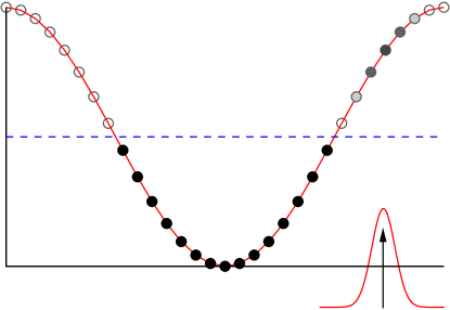
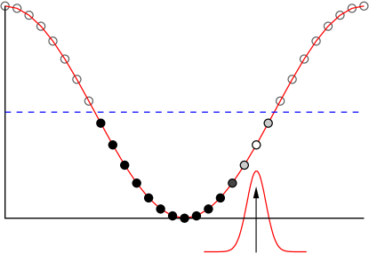
Figure 1: (Colour online) Visualisation of the creation of an electron (left) or a hole (right) by indicating the occupation of single particle levels in the dispersion relation of the non-interacting problem. The dotted line represents the Fermi energy.

In the following figures, we use DMRG White_PRL1992 to generate the ground state $\left|\Psi\right\rangle$ and the excited state $\left|\Psi^{+1}\right\rangle$. For both, the full and the adaptive td-DMRG, the time evolution is performed by a Krylov subspace based evaluation of the time evolution $\left|\Psi^{+1}(t+\Delta t)\right\rangle={\mathrm{e}}^{iH\Delta t}\left|\Psi^{+1}(t)\right\rangle$, for details see Schmitteckert_PRB2004 ; Schmitteckert_HPC2007 ; Boulat_Saleur_Schmitteckert_PRL2008 . The time steps were $\Delta t=0.5$ (in units of time) for both methods.

We use hard-wall boundary conditions in all simulations and all energies are in units of the hopping parameter which is set to 1 in (1). We also calculate the static ground state density $n_{0,\sigma}(x)=\left\langle\Psi\right|c_{x,\sigma}^{\dagger}c_{x,\sigma}\left|\Psi\right\rangle$ at time $t=0$ and form the corresponding charge and spin densities $n_{0,c},n_{0,s}$. Then we plot the quantities $n_{s}(x,t)-n_{0,s}(x)$ and $n_{c}(x,t)-n_{0,c}(x)$. This trick evens out all stationary oscillations already present in the ground state, like the Friedel oscillations resulting from using hard-wall boundary conditions. Additional $2k_{F}$-oscillations resulting from the density distortion of the added excitation are evened out using a three-point average.

In our non-interacting (tight-binding) reference system (1) in figure 2 we create an electron at the real space position $x_{0}=15$ (upper diagram) which travels to the right (lower diagram). The system of size $M=102$ is at half-filling plus one electronic excitation $N_{\uparrow}=51+1$. The $N_{\downarrow}=51$ down-spins are, of course, irrelevant in the non-interacting case and constant in the time evolution. The excitation’s momentum is centred around $k_{0}=\pi/2+0.1$ with width $\sigma_{0}=0.03$. With this width, we ensure that the momentum distribution is far away (compared to the width) from the Fermi surface $k_{0}\sim k_{F}+3\sigma_{0}$ but still as close as possible to the linear regime of the cosine band at $k_{F}$.

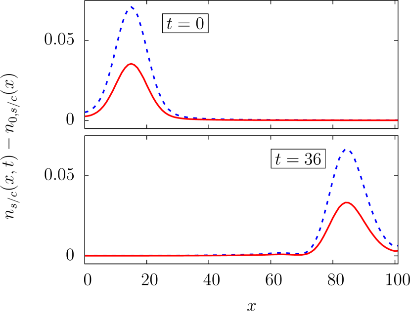
Figure 2: (Colour online) Spin (solid,red) and charge (dashed, blue) densities of a td-DMRG simulation of one additional up-electron over the background of a half-filled tight-binding model for each spin specie. The Gaussian excitation on the left at time $t=0$ (upper diagram) moving to the right at $t=36$ (lower diagram) retains its shape. Averaging is described in the text.

The snapshots at $t=0$ and $t=36$ in figure 2 of spin and charge density serve as a proof-of-concept for the numerics. They show the expected synchronous motion of the electronic excitation with group velocity $v_{G}=1.93\pm 0.02$. A delta-function-shaped excitation in the thermodynamic limit of this system would have a group velocity of $v_{G}(k_{0})\sim 1.99$. Since we are in a finite system, the discretisation and the cut-offs at the Fermi energy and the band edge directly influence the actual shape of the initial density distribution. Also, the non-linearity of the band affects the packet propagation via the width and position of the momentum distribution. The (otherwise perfect time invariant) Gaussian shape is distorted and the packet is slowed down. This system was calculated using $N_{\text{cut}}=1000$ states per DMRG block, applying 10 time steps in the full td-DMRG and keeping $1000$ states for the consecutive adaptive td-DMRG. The discarded entropy never exceeds the order of $10^{-5}$. Comparing to an exact diagonalisation (ED) we define the peak relative error in the densities by

$$|\delta n_{p}(t)|\equiv\max_{x}\left(\frac{n_{\text{ED}}(x,t)-n_{\text{DMRG}}(x,t)}{n_{\text{DMRG}}(x,t)}\right)$$ (5)

This quantity reaches from initial $|\delta n_{p}(0)|=7\cdot 10^{-5}$ peak relative error to $|\delta n_{p}(36)|=7\cdot 10^{-3}$ peak relative error at $t=36$.

Now we repeat the simulation in a Hubbard model bulk system

$$H_{\text{bulk}}=\sum_{\Sigma=\uparrow,\downarrow}H_{\text{tb},\sigma}+U\sum_{x}\left(n_{x,\uparrow}-\frac{1}{2}\right)\left(n_{x,\downarrow}-\frac{1}{2}\right).$$ (6)

While the previous excitation was a superposition of well defined eigenstates in the tight-binding model, it is not clear which eigenmodes are excited by adding/removing an electron from an interacting system. Nevertheless, using the same $c_{\sigma x}^{(\dagger)}$ in equation 3 to create an excitation still results in a Gaussian shape in spin and charge densities (see figure 3), although the corresponding Fourier transformed operators $c_{\sigma k}^{(\dagger)}$ no longer create single particle eigenstates of the system. This time we insert an excitation corresponding to one (up-spin) hole into the ground state of a repulsive particle-hole symmetric Hubbard model (6) with $U=4$ at a filling of $\frac{41}{90}\approx 0.46$ with a central momentum $k_{0}=\pi/2-0.5\sim k_{F}-7\sigma_{0}$ and a width of $\sigma_{0}\sim 0.053$. The calculations were carried out with $N_{\text{cut}}=2500$ states kept per DMRG block in the full and adaptive time dependent DMRG.

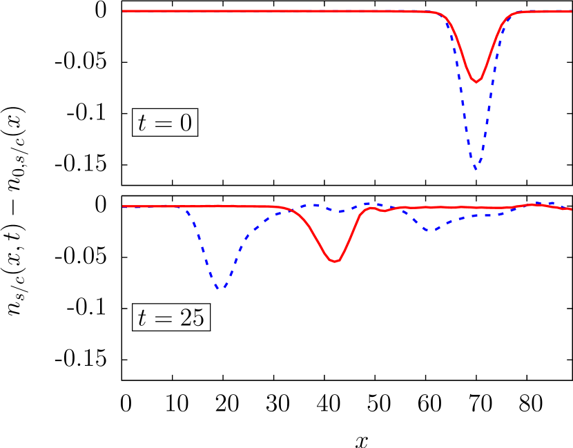
Figure 3: (Colour online) Spin and charge density (see legend of fig. 2) in a Hubbard model at time $t=0$ (upper diagram) and $t=25$ (lower diagram) show spin-charge separation. This is data from a td-DMRG simulation on 90 sites system with $N_{\uparrow}=41-1$, $N_{\downarrow}=41$ electrons and a Hubbard interaction of $U=4$.

One clearly observes SCS driven by the Hubbard interaction between $t=0$ (upper diagram) and $t=25$ (lower diagram). We extract the group velocities from the main peaks to be $v_{S}=1.12\pm 0.05$ and $v_{C}=2.03\pm 0.05$. The velocity is constant through out the simulation and the error stems from the read-off error. The one dimensional Hubbard model can be solved exactly Lieb_Wu_PRL1968 . From the analytic expression by Coll Coll_PRB1974 , the spin and charge velocity of the low energy spinons and holons can be derived as done, e.g. by Schulz Schulz_IJMPB1993 . The excitation’s momentum of $k_{0}$ corresponds to a band filling of $n=0.68$ in units of the hopping. Given the error estimate above, it is accurate enough to read off a charge velocity of $v_{C,\text{one holon}}\sim 2.05$ and $v_{S,\text{one spinon}}\sim 1.15$ (cf. figure 11 of the first paper of Ref. Schulz_IJMPB1993 ). Although we are with 90 sites far from simulating the thermodynamic limit, the group velocities of our spin and charge density fit remarkably well to the Bethe Ansatz results for the velocity of one spinon and one holon. A similar good agreement was found for a spinless Luttinger liquid simulation Schmitteckert_PRB2004 .

Our electronic excitation with a definite momentum $k_{0}$ created a unidirectional running peak in the non-interacting system. Here, however, our initial excitation creates both a right and a left moving density peak in the charge sector. At time $t=25$, the right moving charge peak has already been reflected on the right wall and is located at around $x=60$. The spin density, in contrast, displays predominantely a left moving peak. Finally, there is charge density accumulation trailing the main charge peak and at the location of the spin peak. These might be more complicated features of the interaction or result from the finiteness of the system as in the non-interacting example.

Following the previous line of arguments, it seems reasonable to do a transport setup that uses non-interacting leads as a starting point. We let this excitation travel through an interacting region where SCS occurs and then let the resulting excitations travel again into a non-interacting area. In the starting lead our electronic excitation is well understood. When this excitation travels into the interacting region, we know the momentum and energy of the injected wave packet (one electron or one hole) but the questions arise: what kind of excitation leaves the structure and what can be measured on the opposite (non-interacting) lead?

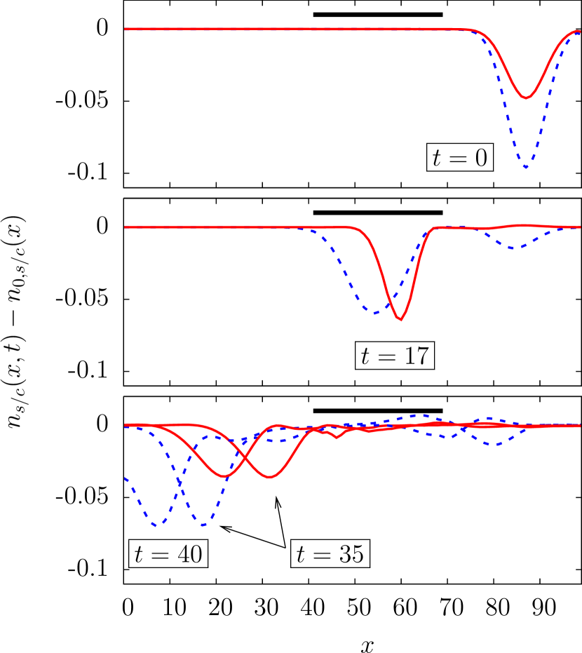
Figure 4: (Colour online) Excitation in a transport experiment: a created hole in the right lead (upper diagram, at $t=0$) passes the interacting nanostructure (black bar) undergoing SCS (central diagram, at $t=17$). At $t=35,40$ (lower diagram) spin and charge densities travel independently with equal velocity in the left lead.

We use a system of $M=100$ sites, split into 41, 29 and 30 sites for the different areas and a total of $N_{\uparrow}=48-1$, $N_{\downarrow}=48$ electrons. The corresponding Hamiltonian reads

$$H_{\text{transport}}=\sum_{\sigma=\uparrow,\downarrow}H_{\text{tb},\sigma}+V_{\mathrm{gate}}\sum_{x=42..70}(n_{x,\uparrow}+n_{x,\downarrow})\\ +U\sum_{x=42..70}\left(n_{x,\uparrow}-\frac{1}{2}\right)\left(n_{x,\downarrow}-\frac{1}{2}\right),$$ (7)

where $H_{\text{tb},\sigma}$ was defined in (1) and $U=2.5$. A gate voltage on the interacting area levels the Fermi surface to a half-integer number of up and down electrons on the structure ($N_{\uparrow}=N_{\downarrow}=12.5$) and minimises reflections into and out of the area (see figure 4). This local chemical potential $V_{\mathrm{gate}}$ in (7) was pre-calculated in a self-consistent way. Thus we have a Hubbard model at $\sim 0.43$-filling in the central (black bar) area and half-filled tight-binding leads. We also chose parameters $k_{0}=0.43\pi-2\sigma_{0}$, $\sigma_{0}=0.03$ to maximise tunnelling while staying as close as possible to a quasi-linear dispersion. The number of states kept was $N_{\text{cut}}=2500$. Figure 4 shows the time evolution of spin and charge densities for several times. There are reflections of charge density at both edges of the structure. They are suppressed by the choice of the chemical potential as discussed above. The majority of spin and charge density transmits through the nanostructure. SCS clearly happens inside the interacting region (central diagram at $t=17$) and SCS remains intact after leaving the interacting area into the opposite lead (lower diagram at $t=35$ and $t=40$). Here spin and charge now travel along separately but again with identical constant velocity.

Conclusions

In our simulation of a microscopic experiment on an interacting nanostructure we saw that the spin and charge excitation of an injected electron can be separated as it is known to happen in one-dimensional interacting systems. The spin and charge separation can be directly observed by a time-resolved measurement of the spin-polarised density. There is no need for spin and charge to recombine to a complete electron (hole) for a measurement of a single electron (hole). Note that the charge and spin excitations in the non-interacting leads are valid excitations of the Fermi liquid. They are not elementary excitations of the Fermi liquid, instead they are a composition of (at least) two excitations of the Fermi liquid. As an example, think of the combinations $(c^{\dagger}_{k,\uparrow}\pm c^{\dagger}_{k,\downarrow})$. However the resulting distribution of separated densities originated from a single particle injection into the Fermi sea. Thereby, we confirm for the Hubbard model, what Safi and Schulz Safi_Schulz_PRB1999 sketched for a low-energy Luttinger liquid transport setup with restricted interaction. It is interesting that our small system already shows the fingerprint of Luttinger Liquid description expected in the thermodynamic limit. Also note that even for highly energetic incoming electrons we find the spin-charge separation, albeit obscured by band effects. With the td-DMRG method even more realistic models, like the extended Hubbard model with a finite next-nearest neighbour interaction could be investigated.

Experimentally, the measurement of the densities would have to happen on a time scale which is set by the Fermi velocity and the length of the interacting system. For nanoscaled systems and metallic excitation velocities tens of Terahertz resolution would be required, which might be achieved using optical techniques. Lowering the Fermi, holon and spinon velocities would enhance the detection possibilities. It is of general interest to know, whether a series of quantum dots or any other strongly correlated system with a much smaller Fermi velocity can provide the ingredients for the realisation of such a transport setup.