Quantum-classical correspondence of the Dirac matrices:
The Dirac Lagrangian as a Total Derivative

Abstract

The Dirac equation provides a description of spin $1/2$ particles, consistent with both the principles of quantum mechanics and of special relativity. Often its presentation to students is based on mathematical propositions that may hide the physical meaning of its contents. Here we show that Dirac spinors provide the quantum description of two unit classical vectors: one whose components are the speed of an elementary particle and the rate of change of its proper time and a second vector which fixes the velocity direction. In this context both the spin degree of freedom and antiparticles can be understood from the rotation symmetry of these unit vectors. Within this approach the Dirac Lagrangian acquires a direct physical meaning as the quantum operator describing the total time-derivative.

I Introduction

Historically, Paul Dirac found the Klein-Gordon equation physically unsatisfactory for the appearence of negative probabilities arising from the second-order time derivative Dirac . Thus he sought for a relativistically invariant Schrödinger-like wave equation of first order in time derivative of the form ($\hbar=c=1$):

$$i\partial_{t}\psi=H\psi\,.$$ (1)

In order to have a more symmetric relativistic wave equation in the 4-momentum components, he also looked for an equation linear in space derivatives i.e. momentum ${\bf P}=-i{\bm{\nabla}}$, so that $H$ takes the form Dirac :

$$H={\bm{\alpha}}\cdot{\bf P}+\beta m\,,$$ (2)

with ${\bm{\alpha}}$ and $\beta$ being independent on space, time and 4-momentum. The condition that Eq. (2) provides the correct relativistic relationship involving energy, rest mass and momentum,

$$E^{2}={\bf p}^{2}+m^{2}\,,$$ (3)

requires that ${\bm{\alpha}}$ and $\beta\equiv\alpha_{4}$ obey the anticommutation rules $\left\{\alpha_{i},\alpha_{j}\right\}=2\delta_{ij}$ ($i=1,4$) weinberg . Dirac found that a set of $4\times 4$ matrices satisfying this relation provides the lowest order representation of the four $\alpha_{i}$. They can be expressed as a tensor product of ($2\times 2$) Pauli matrices $\rho_{i}$ and $\sigma_{i}$ belonging to two different Hilbert spaces: ${\alpha}_{i}=\rho_{1}\sigma_{i}$ ($i=1,3$) and $\beta=\rho_{3}$ Dirac . As a consequence $\psi$ in Eq. (1) is a 4-component wave function. It turns out that ${\bm{\alpha}}$ is the velocity operatorDirac ; Breit . So that $\psi^{\dagger}{\bm{\alpha}}\psi$ is the current density, determining the coupling with the electromagnetic field Dirac ; weinberg ; peskin

This derivation, although straightforward, does not help for a clear physical understanding of the four component wave function and of Dirac matrices. Indeed Richard Feynman in his Nobel lecture pointed out that Dirac obtained his equation for the description of the electron by an almost purely mathematical proposition. A simple physical view by which all the contents of this equation can be seen is still lacking.

The fact that relativistic Dirac theory automatically includes spin leads to the conclusion that spin is a purely quantum relativistic effect originating from the finite dimensional representations of the Lorentz group Fuchs . Nevertheless this interpretation is not generally accepted, e.g. following Weinberg argument (Ref. weinberg Chapter 1) …it is difficult to agree that there is anything fundamentally wrong with the relativistic equation for zero spin that forced the development of the Dirac equation – the problem simply is that the electron happens to have spin $\hbar/2$, not zero. Technically speaking, the homogeneous Lorentz group (in contrast e.g. to the group of rotations) is not a compact group, hence the implementation of this symmetry in quantum mechanics does not need the use of finite dimensional representations. On the contrary, being non compact, it has no faithful finite dimensional representation that is unitary Fuchs ; peskin . Thus the homogeneous Lorentz group is the only group of relativistic quantum field theory acting on multiple-components quantum fields non-unitarily. This rather surprising fact conflicts with a theorem proved by Wigner in 1931 (see Ref. weinberg Chapter 2) which states that any symmetry operation on quantum states must be induced by a unitary (or anti-unitary) transformation.

The conflict is usually overcome, either by regarding the field not as a multicomponent quantum wavefunction but as a classical field peskin , or by pointing out that the fundamental group is not the (homogeneous) Lorentz group but the Poincaré group weinberg . Independently on the point of view, one consequence is that the Hermitean conjugate $\psi^{\dagger}$ of the (four-component) spinor field $\psi$ does not have the inverse transformation property of $\psi$ as requested by quantum mechanics. The rather ad hoc, though generally accepted, solution is to define $\bar{\psi}=\psi^{\dagger}\gamma^{0}$ called the Dirac conjugate of $\psi$, being $\gamma^{0}\equiv\beta$ the time Dirac matrix weinberg ; peskin ; maggiore ; hey .

In this paper we address some naturally arising questions: is there a fundamental compact symmetry group that requires the occurrence of spin? is there a reason why the velocity operator ${\bm{\alpha}}$ of elementary matter particles is a vector made of $4\times 4$ matrices instead of continuous variable operators? is there a simple interpretation of Dirac four-component spinors? Here we discuss how the spin of elementary particles can be understood as a consequence of a rotation symmetry displayed by the kinematic variables describing their space-time motion. Furthermore we show that such rotation symmetry implies the existence of antiparticles.

Before starting our analysis, it is worth pointing out that here we follows the Dirac old fashioned point of view, regarding the Dirac equation as a Schroedinger-like quantum mechanical equation providing the quantum description of a relativistic point-like particle. In contrast the modern view regards the Dirac equation as a classical wave equation describing the $1/2$ spin field. The field is then quantized by means of canonical quantization for relativistic fields weinberg ; peskin .

II Rotations in quantum mechanics

A rotation in classical physics is implemented by a $3\times 3$ orthogonal matrix $R$ which, acting on a given vector ${\bf v}$, gives the rotated vector ${\bf v}^{\prime}=R{\bf v}$. Rotations are a symmetry group whose generator is the angular momentum Goldstein . In quantum mechanics a symmetry transformation is a transformation of the state kets describing the physical system and of the operators $\hat{O}$ in the ket space. The transformation operators ${\hat{D}}(R)$ are unitary and have the same group properties as $R$ (see also supplementary information). The expectation values of the angular momentum operators transform under rotation as classical vectors:

$$\left<J_{k}\right>\to R_{kl}\left<J_{l}\right>$$ (4)

where repeated indices are implicitly summed over Sakurai . The lowest number $N=2j+1$ of dimensions in which the angular momentum commutation relations are realized is $N=2$ (j = 1/2). In this case the angular momentum operators can be represented in terms of the Pauli matrices: $J_{k}=\sigma_{k}/2$. Independently on the physical state in the 2D Hilbert space, they obey the following relationship:

$$\sum_{i}\langle\sigma_{i}\rangle^{2}=1$$ (5)

which is not satisfied by higher order angular momentum operators. Hence Pauli matrices are the best quantum correspondents of classical unit vectors ${\bf\hat{u}}$ (with $\sum_{i}{\hat{u}}^{2}_{i}=1$) Sakurai . If there is any classical physical variable which is described by a unit vector, Pauli matrices provide its natural quantization: ${\hat{u}}_{j}\to\sigma_{j}$, which preserves rotation symmetry and ensures expectation values which maps on the classical values.

III From relativistic kinematics to unit vectors

Let us consider a relativistic point-like particle moving with velocity $\mathbf{v}(t)$ with respect to an observer’s reference frame $K$ Jackson . A possible spacetime worldline trajectory is shown in Fig. 1a. We can consider the Lorentz-invariant quantity

$$d\tau(t)^{2}\equiv dt^{2}-d{\bf x}(t)^{2}\,.$$ (6)

In the instantaneous rest frame $K^{\prime}$ of the particle $d{\bf x}=0$ and hence $d\tau(t)^{2}=dt^{2}$ which admit solutions $d\tau=\pm dt$. The solution $d\tau=dt$ is the one usually presented in the introductory texts on special relativity (see e.g. Jackson ). More recently Costella et al. Costella pointed out that the negative solution provide a classical description of antiparticles in agreement with the Feynman’s interpretation of antiparticles as particles going back in time hey .

Thus from Eq. (6) it follows that:

$$d\tau=\pm\frac{dt}{\gamma(t)}\,,$$ (7)

where $\gamma=(1-v^{2})^{-1/2}$ is the usual Lorentz boost parameter yielding time dilation.

The time $\tau$ is the proper time of the particle. Thus the quantity $d\tau/dt\equiv\dot{\tau}=\pm 1/\gamma(t)$ expresses the rate of change of the proper time with respect to the time $t$ of the reference frame i.e. proper time velocity.

The usual way to describe spacetime trajectories (worldlines) relies on $t-{\bf x}$ Minkowski diagrams, as shown in fig. 1a, where the light cones separates causal events from space-like events. Additional information can be inferred by drawing proper time-time trajectories (timelines) as shown in fig. 1b. The solid line describes the trajectory of a particle with $\dot{\tau}>0$. Trajectories with $\dot{\tau}>0$ can be identified by classical particle motion states, while solutions with $\dot{\tau}<0$ correspond to classical anti-particle states Costella .

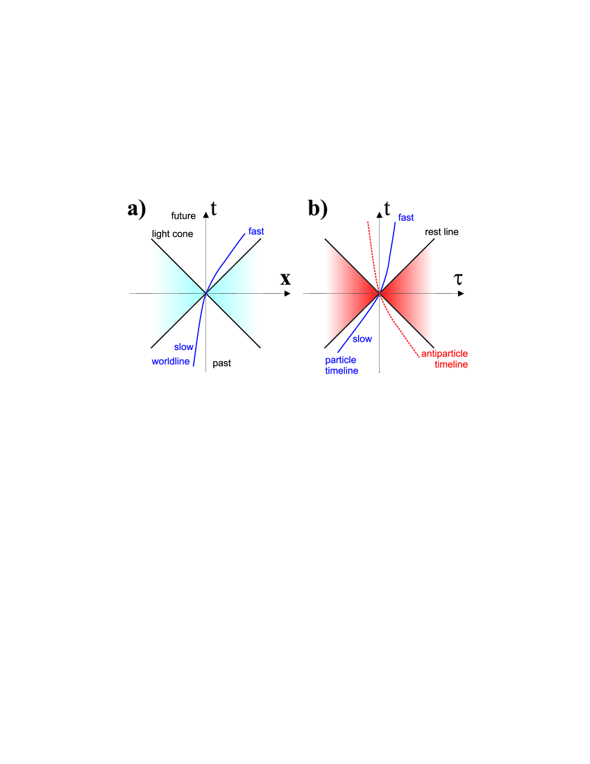
Figure 1: Worldlines of relativistic point-like particle and antiparticles. a) In the usual Minkowski space-time diagram particles and antiparticles worldlines are not distinguished. b) A proper time-time diagram manifests the different kinematics of particles ($\dot{\tau}>0$) and antiparticles ($\dot{\tau}<0$) with respect to an observer’s reference frame.

When attempting to understand the spin and Dirac spinors on a physical ground, the following question arises: are there kinematic variables which can be described as components of unit vectors?

The speed of a particle $v(t)=\left|{\bf\dot{x}}(t)\right|$ is limited (by the speed of light $c=1$) like the component of a unit vector. Additionally the quantity $\dot{\tau}$ can be viewed as the complementary component of this unit vector. Indeed by definition of $\gamma$, it follows that:

$$\left|{\bf\dot{x}}\right|^{2}+\dot{\tau}^{2}=1.\\$$ (8)

Thus we can introduce a convenient unit vector ${\bf\hat{r}}\equiv(\left|{\bf\dot{x}}\right|,0,{\dot{\tau}})$ lying on the $r_{1}r_{3}$ plane (see Fig. 2a) and an angle $\phi$ so that:

$$\left|{\bf\dot{x}}\right|=\sin\phi,\ \dot{\tau}=\cos\phi.\\$$ (9)

A particle changing its kinematic state will move on the unitary circle defined by the angle $\phi$.

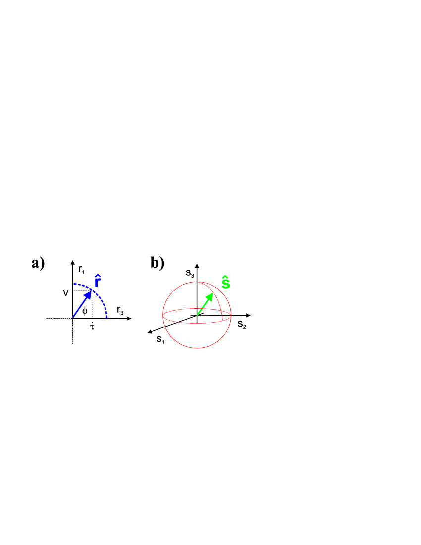
Figure 2: Geometric representations of unit vectors defining the kinematic state of a relativistic point-like particle. (a) The unit vector ${\bf\hat{r}}$ is defined by the modulus of space and proper time velocities. A particle changing its kinematic state will move on the unitary circle defined by the angle $\phi$. (b) The unit vector ${\bf\hat{s}}$ is defined by the spatial direction of velocity and can rotate on the 3D unitary Poincaré sphere.

Figure 2a displays one such kinematic vector with positive components. If the particle is at rest with respect to the reference frame, the vector lies on the $r_{3}$ axis (${\dot{\tau}}=1$). Moreover $\dot{\tau}$ decreases when the particle-speed increases as predicted by special relativity (time dilation).

The unit vector ${\bf\hat{r}}$, besides ${\dot{\tau}}$, is able only to describe the modulus of the particle velocity $v=\left|{\bf\dot{x}}\right|$. The particle velocity is indeed a 3D vector and the direction of ${\bf\dot{x}}$ can be accounted for by one additional 3D unit vector ${\bf\hat{s}}$ providing just the direction of ${\bf\dot{x}}$. Hence the motion state of a particle can be described by a specific couple of unit vectors ${\bf\hat{r}}$ and ${\bf\hat{s}}$:

$${\dot{\tau}}={r}_{3}\,,\hskip 28.45274pt{\bf\dot{x}}={r}_{1}\,{\bf\hat{s}}\,.$$ (10)

Within this approach changes of the particle velocity respect to an inertial frame can be accounted for by rotations of ${\bf\hat{r}}$ in the kinematic plane (changes of the modulus) and rotations of ${\bf\hat{s}}$ (changes of the direction). The unit vector ${\bf\hat{s}}$ can be transformed according to arbitrary 3D rotations around an arbitrary 3D unit vector ${\bf\hat{n}}$:

$$s_{i}\to s_{i}^{\prime}=[{R}_{\bf\hat{n}}(\theta)]_{ij}\,s_{j},$$ (11)

where $\theta$ labels the angle of rotation about ${\bf\hat{n}}$. On the other hand, physical kinematic states ${\bf\hat{r}}$ admit only rotations about the $r_{2}$-axis:

$$r_{i}\to r_{i}^{\prime}=[R^{\prime}_{{\bf j}}(\phi)]_{ij}\,r_{j}\,.$$ (12)

We observe that this rotation symmetry suggests that states obtained rotating ${\bf\hat{r}}$, and ${\bf\hat{s}}$ should be considered as accessible states. In particular ${\bf\hat{r}}$ also describes kinematic states in the second and third quadrant with ${\dot{\tau}}<0$, corresponding to classical antiparticles Costella

From the point of view of classical special relativity, the description in terms of ${\bf\hat{s}}$ and ${\bf\hat{r}}$ appears to be redundant: a given velocity is described by two different states. For example a particle with given velocity along direction ${\bf\hat{d}}={\bf\dot{x}}/\left|{\bf\dot{x}}\right|$ can be described by the unit vectors ${\bf\hat{s}}_{\uparrow}={\bf\hat{d}}$ and ${\bf\hat{r}}_{\uparrow}=(\sin\phi,0,\cos\phi)$ with $\phi=\arcsin\left|{\bf\dot{x}}\right|$, or equivalently by the unit vectors ${\bf s}_{\downarrow}=-{\bf\hat{d}}$ and ${\bf\hat{r}}_{\downarrow}=(\sin\phi^{\prime},0,\cos\phi^{\prime})$ with $\phi^{\prime}=-\phi$. This two-valuedness can be described in terms of the helicity variable $h=({\bf\hat{s}}\cdot{\bf p})/p$. Below we show that this classical twofold degeneracy is indeed the classical correspondent of the helicity states determined by quantum spin. It is worth pointing out that, although the present approach describes a spin-like degree of freedom yet at a classical level, the interaction of a classical particle with the electromagnetic field is not affected by this additional degree of freedom, in contrast to what happens after quantization.

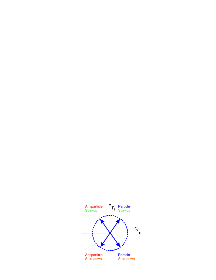
Figure 3: Sections of the velocity space describing the different solutions. Unit vectors in the first and fourth quadrants describe spin up and spin down particles respectively. Unit vectors in the second and third quadrant describe spin up and spin down antiparticles.

Figure 3 provides a clear geometric interpretation of the different kind of kinematic states: the first quadrant contains spin up particles, the second one spin up antiparticles, the third spin down antiparticles and the fourth quadrant spin down particles (see Supplementary Information).

IV From unit vectors to Dirac matrices

As discussed earlier, a quantum mechanical description of unit vectors is obtained replacing the classical vector components with Pauli matrices: $r_{i}\to\rho_{i}$ and $s_{i}\to\sigma_{i}$, where $\rho_{i}$ and $\sigma_{i}$ are now Pauli matrices acting on two different Hilbert spaces $\mathcal{R}$ and $\mathcal{S}$. Hence:

$${\dot{\tau}} = {r}_{3}\to\rho_{3}\otimes I=\beta$$

$${\bf\dot{x}} = {r}_{1}\,{\bf\hat{s}}\to\rho_{1}\otimes{\bm{\sigma}}={\bm{\alpha}}\,,$$ (13)

being $I$ the identity operator in the $s$ space describing the direction of velocity. The ${\bm{\alpha}}$ and $\beta$ are indeed the well-known Dirac matrices in the standard representation Dirac . Thus we find a direct symmetry-driven correspondence showing that ${\bm{\alpha}}$ is the velocity vector operator, and $\beta$ the proper-time velocity operator. In this quantum picture the helicity operator for a particle of given momentum becomes $h=({\bf\sigma}\cdot{\bf p})/p$ in agreement with the Dirac theory peskin and with our classical derivation of helicity states. In summary, at a classical level, the rotation symmetries we introduced describe the correct relativistic kinematics. Furthermore they lead to two possible helicities for a given motion state and the existence of particles with $\dot{\tau}<0$. After quantization, without any other additional assumption, they give rise to the 4-component Dirac spinors fully describing quantum spin and antiparticles with the corresponding expectation value $\langle\beta\rangle<0$. We point out that in this framework the Dirac matrices are derived only on the basis of the fundamental rotation symmetry without any reference to the Dirac equation or to the energy of a relativistic free particle.

At this point it is interesting to show that the energy of a relativistic free particle can be written as observed By Breit as $E={\bf v}\cdot{\bf p}+\dot{\tau}m$. This equation has the same structure of the Dirac Hamiltonian.

V The Dirac Lagrangian as a Total Derivative

A crucial feature of this symmetyry based derivation of the Dirac matrices is that it has been obtained by regarding the position-coordinate and the proper time of the particle on the same footing as functions of the time-coordinate of the reference frame, i.e. we use $t$ as the relevant meter to which compare the dynamical evolution of all other observables (as happens in non-relativistic mechanics). Accordingly if a quantum wavefunction depends on position ${\bf x}$, it should also depend on $\tau$ i.e. $\psi(t,{\bf x},\tau)$. We now consider a particle with such wavefunction and require the conservation of its probability density $\mathcal{D}(t,{\bf x},\tau)\equiv\psi^{*}(t,{\bf x},\tau)\psi(t,{\bf x},\tau)$:

$$\frac{d}{dt}\,\mathcal{D}=\frac{d\psi^{*}}{dt}\psi+\psi^{*}\frac{d\psi}{dt}=0\,.$$ (14)

Stationarity of $\psi$ (and $\psi^{*}$) ensures that a continuity equation holds. In turn if, as in Lagrangian formulations with complex fields, $\psi$ and $\psi^{*}$ are regarded as independent, Eq. (14) implies stationarity of $\psi$ (and of $\psi^{*}$) i.e. $d\psi/dt=0$. Because the time dependence of the wavefunction is both explicit and implicit (through the time dependence of ${\bf x}$ and $\tau$), we have:

$$\frac{d}{dt}\psi=\partial_{t}\,\psi+{\bf\dot{x}}\cdot\partial_{\bf x}\,\psi+{\dot{\tau}}\partial_{\tau}\,\psi\,=0.$$ (15)

Thus the request of stationarity and the crucial symmetry-based quantization Eq. (13), provides a generalized Dirac-like equation:

$$i{\partial}_{t}\psi(t,{\bf x},\tau)=H_{g}\psi(t,{\bf x},\tau)\,,$$ (16)

with

$$H_{g}={\bm{\alpha}}\cdot(-i\partial_{\bf x})+\beta(-i\partial_{\tau})\,.$$ (17)

The corresponding Lagrangian density can be written as

$$\psi^{\dagger}{\cal L}\psi=\psi^{\dagger}i(\partial_{t}+{\bm{\alpha}}\cdot{\partial}_{\bf x}+\beta{\partial}_{\tau})\psi\,.$$ (18)

This Lagrangian operator ${\cal L}$ has a precise physical meaning, being the Hermitean quantum operator describing the total time derivative: $id/dt\to{\cal L}$ after symmetry-based quantization Eq. (13). Equation (17) is more general than the Dirac equation since the mass parameter is now replaced by the internal time momentum operator. Elementary matter particles of given mass can be viewed as eigenstates of this operator. In this case Eq.(17) reduces to the standard Dirac equation. On the other hand, this new degree of freedom offers a chance to shed new light on some fundamental aspects and concepts.

As an example this new degree of freedom could be exploited to discuss charge conservation. Charge conservation is generally accounted by invariance under phase change of a field, Eq. (17) allows the interpretation of this phase change as the consequence of proper time translation applied to an eigenstate of the proper time operator. Charge conservation could thus be viewed as arising from invariance of the Lagrangian under proper time translations.

It is also interesting to address the proper time reversal symmetry $\tau\rightarrow-\tau$. Applying this symmetry to a positive energy solution of Eq. 17 which is also an eigenstate of the proper time momentum (i.e. a particle with fixed mass and charge), we obtain its antiparticle with positive energy and opposite charge, so antiparticle solutions with positive energy emerge without the need for second quantization adjustments.

VI Conclusions

Within the approach here presented, changes of the velocity modulus and direction of a relativistic particle can simply be accounted by rotations of two independent unit vectors. Dirac spinors just provide the quantum description of these rotations. These transformations are able to describe the helicity of a pointlike particle yet at a classical relativistic level, rendering spin a less mysterious degree of freedom. This analysis sacrifies explicit covariance by making explicit rotation symmetry which nevertheless is the fundamental symmetry on which the algebra of the Lorentz group is based. We observe that the addressed rotation symmetries form a compact group hence with unitary finite-dimensional representations as all other symmetry groups in quantum field theory. A feature of this analysis is that it has been obtained by regarding the position-coordinate and the proper time of the particle on the same footing as functions of the time-coordinate of the reference frame, i.e. t is used as the relevant meter to which compare the dynamical evolution of all other observables (as happens in non-relativistic quantum mechanics).

Within this approach we derived the Dirac equation just invoking total stationarity of the wavefunction with respect to the reference time. No assumptions about the classical relativistic energy of a particle or about the quantum operator replacements ($E\to i\partial_{t}$ and ${\bf p}\to-i\partial_{\bf x}$) have been performed. Finally we observe that the quantum replacement $m\to-i\partial_{\tau}$ implies an internal time-energy uncertainty principle $\Delta\tau\,\Delta m$, e.g. as required by a gedanken experiment recently proposed by Aharonov and Rezni Ahranov .

References

- (1) Dirac, P.A.M. The Principles of Quantum Mechanics, (Oxford University Press, Oxford, 1958).
- (2) S. Weinberg, The Quantum Theory of Fields vol. 1: Foundations (Cambridge University Press, Cambridge, 1995).
- (3) G. Breit, Proc. Nat. Acad. Sci. 14, 555 (1928).
- (4) M. E. Peskin and D. V. Schroeder An Introduction to Quantum FIeld Theory (Perseus Books, Reading, MA, 2000).
- (5) J. Fuchs and C. Schweigert, Symmetries, Lie Algebras and Representations (Cambridge University Press, Cambridge, 1995).
- (6) M. Maggiore A modern introduction to quantum field theory (Oxford University Press, Oxford, 2005).
- (7) I. Aitchison and A. J. Hey, Gauge theories in particle physics, 2nd ed. (Adam Hilger, Bristol, 1989).
- (8) R. Feynman in Nobel Lectures, Physics 1963-1970 (Elsevier, Amsterdam, 1972) http://nobelprize.org/nobel_prizes/physics/laureates/1965/feynman-lecture.html.
- (9) Goldstein, H., Poole, C.P., Safko, J.L. Classical Mechanics, 3rd ed. (Addison Wesley, 2001).
- (10) J. J. Sakurai, Modern Quantum Mechanics 2nd ed. (Cambridge University Press, Cambridge, 1995) (Addison Wesley, San Francisco, 1993). .
- (11) Jackson, J.D. Classical Electrodynamics, 3rd ed. (Wiley, New York, 1999).
- (12) Costella, J.P., McKellar, B.H.J., Rawlinson, A.A. Classical antiparticles. Am. Journ. Phys. 65, 835-841 (1997).
- (13) Foldy, L.L. Wouthuysen, S.A. On the Dirac theory of spin 1/2 particles and its non-relativistic limit. Phys. Rev. 78, 29-36 (1950).
- (14) T. L. Kaluza, Sitz. Bal. Akad., 966 (1921).
- (15) O. Klein, Z. Phys. 37, 895 (1926).
- (16) Y. Aharonov, and B. Reznik, Phys. Rev. Lett. 84, 1368 (2000).