Cross-Layer Design of FDD-OFDM Systems based on ACK/NAK Feedbacks

Abstract

It is well-known that cross-layer scheduling which adapts power, rate and user allocation can achieve significant gain on system capacity. However, conventional cross-layer designs all require channel state information at the base station (CSIT) which is difficult to obtain in practice. In this paper, we focus on cross-layer resource optimization based on ACK/NAK feedback flows in OFDM systems without explicit CSIT. While the problem can be modeled as Markov Decision Process (MDP), brute force approach by policy iteration or value iteration cannot lead to any viable solution. Thus, we derive a simple closed-form solution for the MDP cross-layer problem, which is asymptotically optimal for sufficiently small target packet error rate (PER). The proposed solution also has low complexity and is suitable for realtime implementation. It is also shown to achieve significant performance gain compared with systems that do not utilize the ACK/NAK feedbacks for cross-layer designs or cross-layer systems that utilize very unreliable CSIT for adaptation with mismatch in CSIT error statistics. Asymptotic analysis is also provided to obtain useful design insights.

I Introduction

I-A Background and motivation

Cross-layer scheduling has been shown to achieve a significant performance gain in wireless systems as a result of multiuser diversity gain. Most of the existing cross-layer designs heavily rely on either perfect CSIT [6] [13][14] or imperfect [15] [18]/ delayed CSIT [7] [19].

I-A1 Absence of Accurate CSIT and CSIT error statistics

Perfect CSIT is difficult to obtain in practice, especially in FDD systems in which explicit feedback is required. With imperfect CSIT , systematic packet errors would result even if powerful error correction codes are applied. This is because given the imperfect CSIT, there is uncertainty on the instantaneous mutual information at the base station and the scheduled data rate may exceed the instantaneous mutual information, leading to packet errors (channel outage) despite the use of powerful error correction coding. It has been shown [5][20] that packet errors cause significant degradation in cross-layer performance. There are some works to take into account of the imperfect CSIT or limited CSIT feedback in cross-layer design. For example, in [16] [17], the authors studied the cross-layer design with noiseless limited feedback. In [15] [19], the authors studied OFDMA cross layer design with outdated CSIT. However, in all these works, the CSIT obtained is either noiseless (or no delay) or the statistics of the CSIT errors is assumed to be known [7]. However, in practice, the knowledge of CSIT errors statistics such as CSIT error variance and CSIT delay is needed and this is not easy to obtain because it depends on the mobility of the users as well as the multipath profile. It is quite challenging to have a robust cross-layer scheduling solution without the knowledge of CSIT error variance. On the other hand, regardless of the CSIT, there are always ACK/NAK flows between the mobiles (MS) and the basestations (BS). A robust cross-layer scheduling should make the best use of the ACK/NAK information which is embedded in the protocol.

I-A2 Accomodation of mobiles with different receiver capability

Conventional cross-layer design that utilized CSIT to perform resource allocation is essentially an open-loop system because BS cannot determine if the packet is received correctly or not even with the knowledge of CSIT (due to decoding errors). In practice, the system may have heterogeneous mix of mobiles with different capabilities (e.g. some has turbo decoding capability while some only has simple detection capability). To accommodate the heterogeneous mixture of receiver capability in the resource allocation, the BS has to rely on ACK/NAK flows (because the ACK/NAK flows give information about whether a packet can be decoded successfully or not). This closed loop information cannot be obtained in CSIT-based scheduler.

I-A3 Heuristic Approach in existing literature

Recognizing the importance of utilizing the ACK/NAK in the resource allocation at the BS, there are existing works that discuss power control using ACK/NAK feedbacks. However, most of the works either considered power control on a wireless link only as well as utilizing heuristic algorithms or study the performance by simulation. For example, a power adaptation design and performance study utilizing ACK/NAK feedbacks for point-to-point systems have appeared in [21]-[24]. Cross-layer scheduling utilizing ACK/NAK feedbacks was investigated in [9] [10][25]. In particular, power control, rate adaptation and user scheduling for flat fading channels and frequency selective channels were carried out in [9] and [10] respectively whereas a rate adaptation scheme based on ACK/NAK feedbacks was proposed in [25]. The authors proposed a 2-level hierarchy stochastic scheduling algorithm based on learning automata (LA) for an AWGN channel by rate adaptation. Although the algorithm was shown to converge to the true channel state values, the convergence is not proven to maximize the throughput which is of usual practical concern. Moreover, in all these works [9][10][25], the algorithm designs are based on heuristic solutions and it is not clear what the best possible performance from the ACK/NAK information is. Furthermore, the suboptimal solutions obtained have high complexity and is not suitable for real-time implementations. Moreover, in all these existing designs, there is no mechanism to control the per-user packet error rate PER to a given target level. Yet, being able to control the PER of the wireless sessions per user is very important from the requirements of applications (e.g. voice and video codec).

Motivated by all the reasons above, we propose a robust closed-loop cross-layer design for OFDM systems where no explicit CSIT knowledge is needed at the base station. The cross-layer power allocation, user assignment as well as rate allocation are adaptive to the built-in 1-bit ACK/NAK feedbacks [1] [2] [3] from the selected users. Being built in at the link layer of most wireless systems and hence, the ACK/NAK feedbacks add no incremental cost to the proposed closed-loop design. Moreover, since the cross-layer solution is driven by the ACK/NAK feedbacks, it introduces robustness on the cross-layer performance with respect to uncertainty at the CSIT and propagation parameters. These robustness cannot be obtained by utilizing explicit limited CSIT feedback. However, there are several challenges in solving the problem:

I-B Technical Challenges

I-B1 Issues of packet errors

Conventional cross-layer optimization only consider sum ergodic capacity as the optimization objection. Ergodic capacity only considers the b/s/Hz transmitted by the BS regardless of packet errors. As a result, ergodic capacity is a reasonable performance metric only when the packet error is negligible (which is the case with perfect CSIT and very strong coding). However, in our case without CSIT, there is always systematic packet errors (due to channel outage) and this cannot be alleviated by just using strong coding. To accommodate packet errors, we have to use system goodput (b/s/Hz successfully received by the mobiles) as our performance metric. Note that goodput reduces to ergodic capacity in the case of no errors but in general, to deal with goodput, we need to deal with the cdf of mutual information (rather than the first order moment only) and this impose some technique challenges to the problem.

I-B2 Issue of the MDP complexity

While the problem belongs to MDP, it is well-known that there is usually no simple solution (even numerically) using standard value-iteration and policy-iteration solutions (see details in section II). For instance, the MDP belongs to the class of infinite state space and brute-force approach has exponential complexity in the number of time slots $M$ and hence, they could not give useful solutions. Instead of brute-force solution, we exploit some special structure of the OFDM and obtained a low complexity closed-form solution, which is asymptotically optimal for sufficiently small PER target.

I-B3 Asymptotic Performance

As pointed out, all existing solutions are heuristic in nature and studied performance purely by simulations. This is because of the challenging nature of the problem. In this paper, we shall derive some asymptotic properties on the system performance so as to obtain some design insights.

I-C Summary of Contributions

We consider the downlink of a wireless system with a base station and $K$ mobile users over frequency selective fading channels (OFDM). The base station shall adapt the downlink rate, power and user selection in an OFDM system based on the ACK/NAK feedbacks from the mobiles. To take into account of potential packet errors due to channel outage, we consider an average system goodput which measures the number of bits successfully transmitted as our performance measure. The robust cross-layer design is modelled as a Markov Decision Process (MDP) [4] [35] [36] [37] with power, rate and user selection policies as the optimization variables so as to optimize the average system goodput while maintaining a target PER. It is well-known that MDP-based problems [26][27] always require complex value iteration algorithms. However, in this paper, we shall derive a simple closed-form solution for the MDP cross-layer problem which is asymptotically optimal for sufficiently small target PER. The proposed solution has low complexity and is suitable for realtime implementation. It is also shown to achieve significant performance gain compared with systems that do not utilize the ACK/NAK feedbacks for cross-layer designs or cross-layer systems that utilize very unreliable CSIT for adaptation with mismatch in CSIT error statistics. Furthermore, since the ACK/NAK feedbacks are generated by the mobiles based on CRC checking after packet detection, the proposed closed-loop cross-layer scheme is very flexible in the sense that it can automatically accommodate mobiles with different receive sensitivities in the RF or variations in the baseband estimation and decoding algorithms. Hence, the proposed scheme achieve significant goodput gain with built-in robustness against channel fluctuations as well as variations across the capabilities of different mobile receivers.

II A Review on Markov Decision Process

MDP has found applications in ecology, economics and communications engineering since 1950 [28]. MDP is a modeling tool which describes a sequential decision making process. It is used to make the optimal sequence of decisions where outcomes of the problem are partly random and partly depend on such decisions. The advantage of MDP is that it provides a systematic framework for analysis of optimality, existence, dynamics and convergence of solutions.

A complete description of a MDP problem involves a decision epoch, a state space, a control policy, a state transition kernel as well as a reward function. The time line is first divided into decision epochs in which the controller makes decisions on control actions and the system receives rewards at the decision epochs. Specifically, at the $m$-th decision epoch, the system occupies a state $s_{m}\in\mathbb{S}$ where $\mathbb{S}$ denotes the state space. Based on the observation on the causal state sequence $s_{1},...,s_{m}$, the controller takes a control action $\alpha_{m}\in\mathbb{A}$ where $\mathbb{A}$ is the set of actions. A control policy $\pi$ is defined to be the set of actions for all possible state sequence. Based on the action $\alpha_{m}$ and the current state $s_{m}$, the system receives a reward $R(s_{m},\alpha_{m})$ and moves to the next state $s_{m+1}$ according to the state transition probability kernel $P(s_{m},\alpha_{m},s_{m+1})$. The optimization problem is to find the optimal control policy so as to maximize the total rewards: $\arg\max_{\pi}\sum_{m=1}^{M}R(s_{m},\alpha_{m})$. As a result, a MDP problem can be characterized by the tuple $(\mathbb{S},\mathbb{A},P(.,.,.)),R(.,.))$. One reason why the MDP problem is difficult is due to the huge dimensions of the variable, namely the entire policy space $\pi$. As a result, a key step in solving the MDP is known as divide-and-conquer. Specifically, instead of optimizing for the entire problem, it can shown that the MDP can be solved by optimization of actions $\alpha_{m}$ on a per-stage basis.

There has been a lot of in-depth analysis of MDP [28] [29] and different branches of the problem. Different analysis are needed for finite state space problems v.s. infinite state space problems; finite horizon problems v.s. infinite horizon problems; unconstrained MDP v.s. constrained MDP etc. By constrained MDP, we mean that the problem has one or more constraints on the feasible policy space $\pi$. Constrained MDP problems are closely related to communication problems [29] such as power and rate control problems with an average delay constraint [30]; scheduling problems involving routing in ad-hoc networks [32] or handoff problems [31]. For example, in [31], the authors optimized the occurrence of path optimizations for inter-switch handoffs in wireless ATM networks. The expected total cost per call, including the switching/ handoff cost and signaling costs, is modeled as a infinite-horizon semi-Markov decision process [33] with discount rate. This expected total cost is the objective function to be minimized. At each decision epoch, the decision maker can choose to do path optimization or not which is modeled in the action set. Using divide-and-conquer principle, the MDP problem can be solved using value iteration algorithm or policy iteration algorithm [34]. The model is then extended to have QoS constraints.

This paper is outlined as follows. The channel model is firstly presented in section III. In section IV, the problem formulation is given as a cross-layer optimization problem and a MDP problem. The conventional solutions of MDP is provided at the end of section IV. The proposed solution, which is asymptotically optimal, is presented in section V. Simulation results are analyzed in the section VII. Section VIII presents the conclusion.

III Channel Model

We consider a downlink cross-layer scheduling problem in a frequency selective, block fading (in frequency) and quasi static (in time) channel. The bandwidth is divided into $D$ frequency blocks. The fading gain in each frequency block is flat. With the use of OFDM, the fading of each frequency block is independent to other frequency blocks. Also, in the time domain, we assume that the channel remains quasi-static for a period of time $T$ seconds and we call this a time slot. Thus, the fading gains on each frequency block remain the same throughout a time slot. Within a time slot, we send $M$ packets which occupy the same amount of time, a packet slot, $\frac{T}{M}$ seconds. From now on, the names packet slot and slot are used interchangeably. With frequency block fading, there are $N$ frequency sub-carriers in which $\lfloor\frac{N}{D}\rfloor$ frequency sub-carriers having the same fading gains form a block and there are $D$ blocks in total. The fading gain represented by each frequency block is assumed to be independent of the other blocks. The model is summarized in figure 1.

Figure 1: The channel model is represented graphically. In the frequency domain, assume $D=4$ frequency blocks within $N$ subcarriers, there are $\frac{N}{D}$ subcarriers in each frequency block and have the same frequency gains. In the time domain, channel remains unchanged within $T$ seconds: a time slot. $M$ packets are transmitted in a time slot. Each packet consume $\frac{T}{M}$ seconds: a packet slot.

Denote the number of users in the systems by $K$. Each user $k$ sees a vector channel $\bar{h}_{k}=[h_{k,1},\ldots,h_{k,D}]$ where $h_{k,j}$ is the channel power of frequency block $j$ of user $k$. Stacking all vector channels, we have a channel power matrix $H$.

$$H=\left(\begin{array}[]{c}\bar{h}_{1}\\ \bar{h}_{2}\\ \vdots\\ \bar{h}_{K}\end{array}\right)=\left(\begin{array}[]{ccccc}h_{1,1}&h_{1,2}&\cdots&\cdots&h_{1,D}\\ h_{2,1}&h_{2,2}&\cdots&\cdots&h_{2,D}\\ \vdots&\ddots&&&\vdots\\ h_{K,1}&h_{K,2}&&\ddots&h_{K,D}\\ \end{array}\right)$$ (1)

Note that each entry $h_{k,d}$ is exponentially distributed with unit mean and variance. Denote the ACK/NAK feedback from each user $k$ during packet slot $m$ by $v_{k,m}$. Then,

$$v_{k,m}=\left\{\begin{array}[]{ll}1,&\hbox{ACK is received from user $k$ in slot $m$;}\\ 0,&\hbox{NAK is received from user $k$ in slot $m$.}\\ \end{array}\right.$$ (2)

where ACK is received when the packet $m$ is successfully decoded and NAK is received when the packet $m$ has error.

Figure 2: Closed Loop Cross-Layer Scheduler. The user, power and rate optimization at the BSs is solely based on the 1-bit feedbacksfrom MSs.

The closed-loop cross-layer scheduler is as shown in figure 2. There are three optimization parameters, namely the user selection $a_{m}$ , power level $p_{m}$ and rate $r_{m}$ . The parameters are determined for each packet $m$. At the receiver side, each user $k$ would decode the packet and send a 1-bit ACK/NAK feedback $v_{k,m}$ to the transmitter. In $m$-th packet slot, the maximum achievable rate in bits is

$$c(p_{m},\bar{h}_{a_{m}})=\frac{NT}{DM}\sum_{d=1}^{D}\log_{2}(1+\frac{p_{m}h_{a_{m},d}}{N})$$ (3)

where noise power is normalized to be one.

Now, we can rewrite equation (2) mathematically,

$$v_{k,m}=\left\{\begin{array}[]{ll}1,&r_{m}\leq c(p_{m},\bar{h}_{a_{m}});\\ 0,&r_{m}\geq c(p_{m},\bar{h}_{a_{m}}).\\ \end{array}\right.$$ (4)

In high SNR environment, the maximum bits per packet slot in equation (3) can be approximated by

$$c(p_{m},\bar{h}_{a_{m}})=\frac{NT}{DM}\sum_{d=1}^{D}\log_{2}(1+\frac{p_{m}h_{a_{m},d}}{N})$$

$$\underset{highSNR}{\longrightarrow}\frac{NT}{DM}\left(\sum_{d=1}^{D}\left(\log_{2}\left(\frac{p_{m}}{N}\right)\right)+\log_{2}(X_{a_{m}})\right)$$

$$=c(p_{m},X_{a_{m}})$$ (5)

where $X_{k}=\prod_{d=1}^{D}h_{k,d}$. This approximation significantly reduces the complexity of the system as the D-dimensional channel power gain vector is replaced by a scaler. In figure 3, we show the difference between the maximum bits per packet slot and its approximation in (III). The approximation error is less than 2% when the SNR is around 10dB.

Figure 3: Rate difference between mutual information and its approximation in (III). The difference is less than 2% in common operating region, between 10 to 30 dB.

Define the cumulative density function (CDF) of the random variable $X_{k}$ to be

$$\phi(\chi)=Pr(X_{k}\leq\chi)$$ (6)

which can be computed offline. Note that $X_{k}$ is unknown to the transmitter which updates the set of all possible values of $X_{k}$ in each packet slot $m$ by the feedback $v_{k,m}$. The set of all possible values $X_{k}$, based on information received through feedbacks before packet slot $m$, is

$$\mathbb{X}_{k,m+1}=\left\{\begin{array}[]{ll}\mathbb{X}_{k,m}\bigcap\left\{X_{k}:c(p_{m},X_{k})\geq r_{m}\right\},&v_{k,m}=1;\\ \mathbb{X}_{k,m}\bigcap\left\{X_{k}:c(p_{m},X_{k})<r_{m}\right\},&v_{k,m}=0.\\ \end{array}\right.$$ (7)

For example, at packet slot 1, $m=1$, the set of real channel power gains for $\mathbb{X}_{k,1}$ is all real numbers $\mathbb{R}^{+}$. A pair of power and rate $(p_{1},r_{1})$ is selected. A packet is broadcasted with power $p_{1}$ and rate $r_{1}$. At the end of packet slot 1, ACK/NAK feedbacks $v_{k,1}$ for all users $k$ are received. $\mathbb{X}_{k,2},\forall k$ are then updated using (7). At the end of packet slot 2, $\mathbb{X}_{k,3}$ are updated accordingly and so on. Note that the set $\mathbb{X}_{k,m}$, as described in (7), would solely depend on the causal power allocation, rate allocation and ACK/NAK feedbacks from the users.

IV Problem Formulation

This section is targeted to reveal the mathematical description of the optimization problem. The problem is best explained by first writing down the optimization variables which are the power, rate and user selection policies defined in the following. We would then provide the mathematical expression of the system goodput which is the optimization objective in this paper. A problem statement and its corresponding mathematical representation are provided. A subsection is given here to explain the transformation of the optimization problem to a MDP problem.

IV-A Problem formulation as a cross-layer optimization problem

For simplicity, denote the causal user assignments, rate sequence and power sequence from slots 1 to $m-1$ by $A_{m}=(a_{1},a_{2},\ldots,a_{m-1}),$ $R_{m}=(r_{1},r_{2},\ldots,r_{m-1})$ and $P_{m}=(p_{1},p_{2},\ldots,p_{m-1})$ respectively. Also, denote the causal ACK/NAK feedbacks for slots 1 to $m-1$ from all users by the matrix $V_{m}$

$$V_{m} = \left(\begin{array}[]{ccccc}v_{1,1}&v_{1,2}&\cdots&\cdots&v_{1,m-1}\\ \vdots&\ddots&&&\vdots\\ v_{K,1}&v_{K,2}&&\ddots&v_{K,m-1}\\ \end{array}\right)$$ (11)

$$= \left(\begin{array}[]{c}\bar{v}_{1}^{m}\\ \vdots\\ \bar{v}_{K}^{m}\\ \end{array}\right)=\left(\bar{v}^{1},\bar{v}^{2},\ldots,\bar{v}^{m-1}\right)$$ (15)

Definition 1 (Power Allocation Policy)

A power allocation policy

$$\mathcal{P}=\left\{\left(p_{m}\right)_{V_{m}}:\sum_{m=1}^{M}p_{m}=P_{0}\right\}$$ (16)

is defined as the set of all power allocation at the $m$-th packet slot where $m\in[1,M]$. The subscript notation $(.)_{V_{m}}$ denotes that the power allocation at the $m$-th packet slot is a function of the ACK/NAK feedbacks up to the $(m-1)$-th packet slot $V_{m}$. The power allocation policy $\mathcal{P}$ is restricted by the total power constraint $P_{0}$.

Similarly, we define the rate allocation policy and user selection policy.

Definition 2 (Rate Allocation Policy)

A rate allocation policy

$$\mathcal{R}=\left\{(r_{m})_{V_{m}}:r_{m}\in\mathbb{R}^{+}\right\}$$ (17)

is defined as the set of all rate allocation at $m$-th packet slot where $m\in[1,M]$ and $\mathbb{R}^{+}$ is the set of all positive real numbers. The policy is determined by causal ACK/NAK feedbacks up to slots $m-1$.

Definition 3 (User Selection Policy)

A user selection policy

$$\mathcal{A}=\left\{(a_{m})_{V_{m}}:a_{m}\in\{1,\ldots,K\}\right\}$$ (18)

is defined as the set of all user selection at $m$-th packet slot where $m\in[1,M]$. The policy is determined by the causal ACK/NAK feedback sequences up to slots $m-1$. The user selection at $m$-th packet slot $a_{m}$ denotes the index of user selected.

Let the feedback of user $a_{m}$ at packet slot $m$ in time slot $z$ be $v_{a_{m},m}(z)$. The number of packet errors in time slot $z$ equals to the sum of packet errors of the $M$ packets sent within time slot $z$: $\sum_{m=1}^{M}(1-v_{a_{m},m}(z))$. The total number of packet errors in $Z$ time slots is $\sum_{z=1}^{Z}\sum_{m=1}^{M}(1-v_{a_{m},m}(z))$. Thus, the packet error rate averaged over time slots is

$$P_{e}=\lim_{Z\rightarrow\infty}\frac{1}{MZ}\sum_{z=1}^{Z}\sum_{m=1}^{M}(1-v_{a_{m},m}(z)).$$ (19)

As the channel gain remains quasi-static within a time slot and is independent of that in other time slot, the averaged packet error rate can be written as the expectation of number of packet errors within a time slot over channel realizations.(We drop the notation of time slot $z$)

$$P_{e}=\mathbf{E}_{H}\frac{1}{M}\sum_{m=1}^{M}(1-v_{a_{m},m})$$ (20)

where $\mathbf{E}_{H}(.)$ denotes expectation over the random variable $H$.

Note that the packet error rate can be simplified as follows.

$$P_{e}=Pr(c(p_{m},X_{a_{m}})<r_{m})$$ (21)

The average system goodput $\bar{G}$ (averaged over ergodic samples of time slots) is given by:

$$\bar{G}\left(\mathcal{P},\mathcal{R},\mathcal{A}\right) = \mathbf{E}_{H}\left\{\sum_{m=1}^{M}v_{a_{m},m}r_{m}\right\}$$ (22)

$$= \sum_{m=1}^{M}Pr(c(p_{m},X_{a_{m}})>r_{m})r_{m}.$$

In most wireless systems, a target packet error rate (PER) is assigned due to various application requirements. Let $\epsilon$ be that PER. For example, the PER, $\epsilon$, is of the order of $10^{-2}$ for voice applications. The relation between $\mathbb{X}_{k,m}$ and $\epsilon$ (III) is given by

$$1-\epsilon = Pr(c(p_{m},X_{a_{m}})\geq r_{m}|\mathbb{X}_{a_{m},m})$$ (23)

$$= Pr(X_{a_{m}}\geq\theta_{m}|\mathbb{X}_{a_{m},m})$$

where

$$\theta_{m}=\left(\frac{N}{p_{m}}\right)^{D}2^{\frac{r_{m}DM}{NT}}.$$ (24)

To conclude, the cross-layer optimization problem can be formulated as

Problem 1 (Cross-layer formulation)

Determine the optimal power allocation policy $\mathcal{P}$, rate allocation policy $\mathcal{R}$ and user assignment $\mathcal{A}$ so as to maximize the average system goodput $\bar{G}(\mathcal{P},\mathcal{R},\mathcal{A})$ subject to the target PER requirement $1-\epsilon=Pr\left(X_{a_{m}}\geq\theta_{m}|\mathbb{X}_{a_{m},m}\right)$ and the total power constraint $\sum_{m=1}^{M}p_{m}\leq P_{0}$.

The optimization problem above is difficult to solve due to the huge dimension of variables involved. Yet, we shall illustrate below that the total system goodput $\bar{G}$ can be expressed recursively and hence, the problem above can be expressed as a Markov Decision Problem. Define $F_{m}(\bar{P}_{m},W_{m-1})$ to be the maximized goodput sum from slot $m$ to $M$ (from packet slot $m$ to the last packet slot) subject to power constraint $\bar{P}_{m}$ and causal power allocations, rate allocations and feedbacks from users i.e.

$$F_{m}(\bar{P}_{m},W_{m-1})=\underset{\mathbf{p}_{m},\mathbf{r}_{m},\mathbf{a}_{m}}{max}\mathbf{E}_{H}\left\{\sum_{i=m}^{M}v_{a_{i},i}r_{i}\right\}$$ (25)

where $W_{m-1}=\left(V_{m-1},A_{m-1},\Theta_{m-1}=(\theta_{1},\ldots,\theta_{m-1})\right)$ and $\mathbf{p}_{m}$ denotes the vector of power allocation from $p_{m}$ to $p_{M}$. Similar notations apply to $\mathbf{r}_{m}$ and $\mathbf{a}_{m}$. The maximization is subject to the PER requirement $Pr(X_{a_{m}}\geq\theta_{m}|\mathbb{X}_{a_{m},m})=1-\epsilon$ and the total power constraint $\sum_{i=m}^{M}p_{i}\leq\bar{P}_{m}$. We first have the following lemma about $F_{m}(\bar{P}_{m},W_{m-1})$.

Lemma 1

$F_{m}(\bar{P}_{m},W_{m-1})$ can be espressed recursively as

$$F_{m}(\bar{P}_{m},W_{m-1})$$

$$= \underset{p_{m},r_{m},a_{m}}{max}\left\{(1-\epsilon)r_{m}+\mathbf{E}_{V_{m}}\left[F_{m+1}(\bar{P}_{m}-p_{m},W_{m})\right]\right\}.$$

Proof:

See subsection IX-A in appendix. ∎

Note that the maximization variables are $p_{m},r_{m},a_{m}$, the power, rate and user selection in packet slot $m$, instead of the selections from slot $m$ till the last slot. As a result, this facilitate the divide-and-conquer approach to the original optimization problem in (1).

From (22), the maximized system goodput is

$$\bar{G}^{*}(\mathcal{P},\mathcal{R},\mathcal{A})=\underset{\mathbf{a}_{m},\mathbf{p}_{m},\mathbf{r}_{m}}{max}\sum_{m=1}^{M}\mathbf{E}_{H}\left\{v_{a_{m},m}\right\}r_{m}.$$ (27)

By definition of $F_{m}$ in equation (25), the optimized goodput is

$$\bar{G}^{*}(\mathcal{P},\mathcal{R},\mathcal{A}) = F_{1}(P_{0},W_{0})$$ (28)

subject to $$\sum_{m=1}^{M}p_{m}\leq P_{0}$$

$$Pr(X_{a_{m}}\geq\theta_{m}|X_{a_{m}}\in\mathbb{X}_{a_{m},m})=1-\epsilon$$

$$\theta_{m}=\left(\frac{N}{p_{m}}\right)^{D}2^{\frac{r_{m}DM}{NT}}$$

where $W_{0}$ is a empty set. As a result, the optimized system goopdut $\bar{G}^{*}(\mathcal{P},\mathcal{R},\mathcal{A})=F_{1}(P_{0},W_{0})$ can be obtained recursively from equation (1). We shall eleborate the recursive solution in the following sections.

IV-B Problem Formulation as a Markov Decision Process

As explained in Section II, a MDP problem is characterized by the tuple $(\mathbb{T},\mathbb{S},\mathbb{A},P(s,\alpha,s^{\prime}),R(s,\alpha))$. In our case, the decision epochs of the base station $\mathbb{T}=\{1,2,...,M\}$ corresponds to the scheduling slots. In the following, we shall discuss the association of our cross-layer optimization problem with the MDP tuple, namely the state space $\mathbb{S}$, action space $\mathbb{A}$, state transition kernel as well as the per-stage reward function. Based on that, we shall formally recast the problem into an MDP.

• State Space Association With $\Theta_{m}=[\theta_{1},\ldots,\theta_{m}]$, define $U(\Theta_{m},\bar{v}_{k}^{m})$ and $L(\Theta_{m},\bar{v}_{k}^{m})$ to be the upper bound and lower bound of CSI which is some information gathered by the ACK/NAK feedbacks $\bar{v}_{k}^{m}$ and $\theta_{m}$ in equation (24). The state space, $\mathbb{S}$, is a collection of the following vectors $s$.

  $$s=(L(\Theta_{m},\bar{v}_{k}^{m}),U(\Theta_{m},\bar{v}_{k}^{m}),\theta_{m},\bar{P}_{m},\bar{R}_{m},\vec{s}^{(ACK)},\vec{s}^{(NAK)})$$ (29)

  where $\bar{P}_{m}$ is the remaining power; $\bar{R}_{m}$ is the sumrate from slot $m$ to $M$, $\vec{s}^{(ACK)}$ and $\vec{s}^{(NAK)}$ are the pointers to the states if ACK:$v_{m}=1$ and NAK: $v_{m}=0$ respectively.

  The CSI can take all possible real values and therefore make the state space $\mathbb{S}$ infinite. However, as illustrated in an example in the following subsection, the decision tree built by state transitions in our problem is a lot smaller in size.

• Action Space and Policy Association The action taken at each state $s$ consists of the selection of power $p_{m}$, transmission rate, $r_{m}$, and the user selection, $a_{m}$. The set of possible actions $\mathbb{A}$ at every state $s$ is independent of decision epoch m and it is given by:

  $$\mathbb{A}=\mathbb{A}_{s,m}=\left\{(p_{m},r_{m},a_{m})\in\right.$$ (30)

  $$\left.\left\{p\in\mathbb{R}^{+}:p\leq P_{0}\right\}\times\mathbb{R}^{+}\times\left\{1,\ldots,K\right\}\right\}.$$

• State Transition Kernel Association The transition probability $P(s,\alpha,s^{\prime})$ is a real value function which maps $\left\{\mathbb{S}\times\mathbb{A}\times\mathbb{S}\right\}$ to $[0,1]$. In our case, the probability of going from state $s$ to state $s^{\prime}$ by action $\alpha\in\mathbb{A}$ is time invariant.

  In each decision epoch, $m$, a selection of actions, $\alpha_{m}$, takes place, meaning that the base station selects the power $p_{m}$ and the transmission rate $r_{m}$ to user $a_{m}$. After every user $k$ receives the packet, each of them would decode the packet header and transmit a 1-bit feedback to base station, $v_{k,m}$. This 1-bit feedback carries the information of ACK (1) or NAK (0). The transition probability captures the probability of such ACK (1) or NAK (0) and would take the system to a different state. For instance, the current state is denoted by $s$; the state after receiving ACK $s^{a}$; the state after receiving NAK $s^{n}$. The probability of receiving ACK is $\mathcal{P}_{a}$ and that of NAK is $1-\mathcal{P}_{a}$. The action taken is $\alpha$. We have

  $$P(s,\alpha,s^{a})=\mathcal{P}_{a};$$ (31)

  $$P(s,\alpha,s^{n})=1-\mathcal{P}_{a}.$$ (32)

  And

  $$\sum_{s^{\prime}\in\mathbb{S}}P(s,\alpha,s^{\prime})=1$$ (33)

  The state transition probability is described in equation (31)

  $$P(s,\alpha,s^{\prime})=P(\theta_{m+1}=\mathit{\theta}^{\prime}|\theta_{m}=\mathit{\theta},\alpha_{m}=\alpha)=\begin{cases}\epsilon,&Pr(X_{k}>\mathit{\theta}^{\prime}|X_{k}>L(\Theta_{m},\bar{v}_{k}^{m}),X_{k}<U(\Theta_{m},\bar{v}_{k}^{m}))=\epsilon\\ 1-\epsilon,&Pr(X_{k}>\mathit{\theta}^{\prime}|X_{k}>L(\Theta_{m},\bar{v}_{k}^{m}),X_{k}<U(\Theta_{m},\bar{v}_{k}^{m}))=1-\epsilon\\ 0&\text{otherwise.}\end{cases}$$ (31)

  $$P(s,\alpha,s^{\prime})=\begin{cases}\epsilon,&\phi(\theta_{m+1}=\mathit{\theta}^{\prime})=(1-\epsilon)\phi(U(\Theta_{m},\bar{v}_{k}^{m}))+\epsilon\phi(L(\Theta_{m},\bar{v}_{k}^{m}))\\ 1-\epsilon,&\phi(\theta_{m+1}=\mathit{\theta}^{\prime})=\epsilon\phi(U(\Theta_{m},\bar{v}_{k}^{m}))+(1-\epsilon)\phi(L(\Theta_{m},\bar{v}_{k}^{m}))\\ 0&\text{otherwise.}\end{cases}$$ (32)

  $$P(s_{m},\alpha,s_{m+1})=\begin{cases}\epsilon,&\phi(\theta_{m+1})=(1-\epsilon)\phi(U(\Theta_{m},\bar{v}_{k}^{m}))+\epsilon\phi(L(\Theta_{m},\bar{v}_{k}^{m}))\\ 1-\epsilon,&\phi(\theta_{m+1})=\epsilon\phi(U(\Theta_{m},\bar{v}_{k}^{m}))+(1-\epsilon)\phi(L(\Theta_{m},\bar{v}_{k}^{m}))\\ 0&\text{otherwise.}\end{cases}$$ (33)

  in which $\mathit{\theta}^{\prime}$ is the third element in $s^{\prime}$ and $\mathit{\theta}$ is the third element in $s$. The upper and lower bound of CSI would be modified according to the ACK/NAK feedbacks received. After updating the bounds, the probability of ACK, which is equal to the probability of the event that the channel power $X_{k}$ lies between the lower bound and state $\mathit{\theta}^{\prime}$, has to equal $1-\epsilon$, as dictated by the error constraint. Evaluate the probability, we have equation (32).

• Per-stage Reward To decide which actions in $\mathbb{A}$ should be carried out, we would need a decision rule $d_{m}$. The decision rule $d_{m}$ is a history-dependent function. Define the history $\delta_{m}$ to be a vector of past states, actions and feedbacks.

  $$\delta_{m}=[s_{1},\alpha_{1},\ldots,s_{m-1},\alpha_{m-1},s_{m}]$$ (34)

  The recursive relation is therefore

  $$\delta_{m}=[\delta_{m-1},\alpha_{m-1},s_{m}].$$ (35)

  Denote the set of all histories by $\Delta_{m}$. Note that

  $$\Delta_{1} = \mathbb{S}$$ (36)

  $$\Delta_{2} = \mathbb{S}\times\mathbb{A}\times\mathbb{S}$$

  $$\vdots$$

  $$\Delta_{m} = \mathbb{S}\times\mathbb{A}\times\cdots\times\mathbb{S}$$

  $$= \Delta_{m-1}\times\mathbb{A}\times\mathbb{S}$$

  The history dependent rule $d_{m}$ maps $\Delta_{m}$ to $\mathbb{A}$.

  A control policy is a plan specified by a sequence of decision rules. A control policy $\pi$ is

  $$\pi=(d_{1},d_{2},\ldots,d_{M}),\;\;d_{i}\in\Delta_{i},i=1,\ldots,M$$ (37)

  The per-stage reward function is

  $$R(s_{m},\alpha_{m})=\left\{\begin{array}[]{cc}P(s_{m},\alpha,s_{m+1,a})r_{m}&if\;v_{m}=1;\\ 0&if\;v_{m}=0;\end{array}\right.$$ (41)

  where $s_{m+1,a}$ denotes the state at slot $m+1$ if $s_{m}$ is reached at slot $m$ and action $\alpha_{m}$ is taken.

Problem 2 (The MDP formulation)

The MDP problem is defined as a maximization problem of the reward function, in our case, the system goodput $F_{1}(P_{0},W_{0})$. Thus, the problem statement is, with slightly abuse of notation

$$\underset{\pi}{max}\left\{\sum_{m=1}^{M}R(s_{m},\alpha_{m})\right\}$$ (42)

such that $\forall m=1,\ldots,M,s_{m},s_{m+1}\in\mathbb{S}$, $\alpha_{m}\in\mathbb{A},r_{m}\in\mathbb{R}^{+}$ and equation (33) is satisfied.

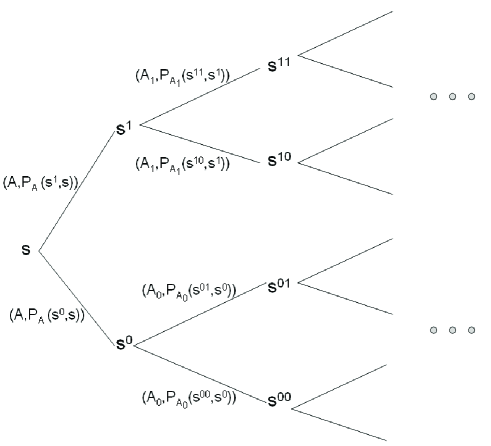
Figure 4: A state transition diagram example. With only 2 possible outcomes at each state (node), the state space (the number of nodes) increases exponentially, hence the problem size.

IV-C A State Transition Example

To illustrate the state transition of a MDP, a state transition diagram assigned with an initial state is given in figure 4 by only drawing transition branches corresponding to the tuples of scheduled action and the corresponding non-zero transition probability. Note that this diagram only shows a fragment of the whole decision tree because there are more than one possible initial state.

The decision tree has $O(|\theta_{m}|)^{3}\times 2^{M}$ elements, where $|\theta_{m}|$ is the number of values $\theta_{m}$ can take. In other words,

$$|\mathbb{S}|=O(|\theta_{m}|)^{3}).$$ (43)

There are $|\theta_{m}|$ possible values of the lower bound $L(\Theta_{m},\bar{v}_{k}^{m})$. For example, $L(\Theta_{m},\bar{v}_{k}^{m})\in\left\{y_{1},\ldots,y_{|\theta_{m}|}\right\}$ where $y_{b}<y_{b+1}$. For each value of lower bound $y_{b}$, there are $|\theta_{m}|-b-1$ values of $U(\Theta_{m},\bar{v}_{k}^{m})$ and $\theta_{m}$. Thus, the total number of possible states is $1^{2}+2^{2}+\ldots+|\theta_{m}|^{2}=O(|\theta_{m}|^{3})$.

With either positive or negative feedbacks, each state can only branch to 2 possible next states. Assume that we start on one of these states. The number of possible descendents would be equal to the sum of the series $1+2+2^{2}+2^{3}+\ldots+2^{M-1}$ which is $2^{M}$. Thus, the total number of nodes in the tree is $O(|\theta_{m}|)^{3}\times 2^{M}$.

Denote the elements in the state space $\mathbb{S}$ by

$$\mathbb{S}=\left\{s,\{s^{0},s^{1}\},\{s^{00},s^{01},s^{10},s^{11}\},\ldots,\{s^{q_{M-1}}\}\right\}$$ (44)

where $q_{M-1}$ denotes any possible binary sequence of length $M-1$. The binary sequence represents the causal ACK or NAK feedbacks received. For example, state $s^{00}$ represents that 2 NAKs have been received and state $s^{101}$ represents that the first and the third transmission are correct and the second transmission or guess is incorrect. The state $s^{q_{i}}$ is at the $i$-th level of the tree which means the $(i+1)$-th packet transmission (with the root being the zeroth level). In the diagram, only transitions with non-zero probability are drawn. The transition probability corresponding to action $A_{q_{i}}\in\mathbb{A}$ from state $s^{q_{i}}$ to state $s^{[q_{i},0]}$, meaning that a NAK is received at $(i+1)$-th packet transmission, is denoted by the probability $P\left(s^{q_{i}},A_{q_{i}},s^{[q_{i},0]}\right)$. At each state $s^{q_{i}}$, there are two possible transition branches

$$ACK:$$ (45)

$$\left(A_{q_{i}},P\left(s^{q_{i}},A_{q_{i}},s^{[q_{i},1]}\right)\right)=\left((p_{i+1},r_{i+1},a_{i+1}),1-\epsilon\right)$$

$$NAK:$$ (46)

$$\left(A_{q_{i}},P\left(s^{q_{i}},A_{q_{i}},s^{[q_{i},0]}\right)\right)=\left((p_{i+1},r_{i+1},a_{i+1}),\epsilon\right).$$

IV-D Conventional Solutions of MDP

A conventional solution to a MDP consists of backward and forward recursions. The backward recursions set up a huge searching tree/ table which would involves dynamic programming. In the forward recursions, the system states evolve through the tree. Here we adopted the Finite Horizon-Policy Evaluation Algorithm in [28] for the backward recursion.

Algorithm 1 Conventional Finite Horizon- Policy Evaluation Algorithm

1:Each node in the tree consists of following fields: $(L,U,\theta_{m},\bar{P}_{m},\bar{R}_{m},\vec{s}^{(ACK)},\vec{s}^{(NAK)})$.

2:Initialization: $m\leftarrow M$, $\forall L,U,p_{M},\theta_{M}$

3:$F_{M}^{*}(p_{M},\delta_{M})=\underset{d_{M}(\delta_{M})}{max}Pr(c(p_{M},\theta_{M})>r_{M})r_{M}$

4:if $m=1$, stop. Otherwise, go to step 4.

5:$m\leftarrow m-1$, $\forall s_{m},p_{m},\bar{P}_{m},L,U$

6:Evaluate $F_{m}^{*}(\bar{P}_{m},\delta_{m})=\underset{d_{m}(\delta_{m})}{max}\left\{P(s_{m},\alpha,s_{m+1})r_{m}\right.$ $+P(s_{m},\alpha,s_{m+1})F_{m+1}^{*}(\bar{P}_{m}-p_{m},\delta_{m}|v_{a_{m},m}=1)$ $\left.+(1-P(s_{m},\alpha,s_{m+1}))F_{m+1}^{*}(\bar{P}_{m}-p_{m},\delta_{m}|v_{a_{m},m}=0)\right\}$ such that the constraints in equation (33) are satisfied and $P(s_{m},\alpha,s_{m+1})=1-\epsilon$

7:$(p_{m},a_{m},r_{m})$ are given by $d_{m}(\delta_{m})$ obtained in step 4.

8:$\bar{R}_{m}=F_{m}^{*}(\bar{P}_{m},\delta_{m})$ which is the accumulated rate of this node and its descendents.

9:$\vec{s}^{ACK},\vec{s}^{NAK}$ are computed in (33)

After building up a table in backward recursion using algorithm 1, from $m=M\rightarrow 1$, we established a large binary tree with each node represents a particular estimate of channel power and each branch corresponds to an ACK/NAK feedback. Each path from the root to the leaves corresponds to a sequence of estimates and the corresponding feedbacks. In Online Evolution (algorithm 2), we read this tree from the root and traverse down to the leaves. Each packet is transmitted with parameters marked in that node and a new node is reached according to the ACK/NAK feedbacks.

Algorithm 2 Conventional Online State Evolution Algorithm

1:Set $m=1$ and start state

2:$s=(0,\infty,\theta_{m},P_{0},\bar{R}_{m},\vec{s}^{(ACK)},\vec{s}^{(NAK)})$

3:where $\bar{R}_{m}$ is the maximum among the nodes with $L=0,U=\infty$.

4:If $m=M+1$, stop, otherwise go to step 3.

5:Transmit packets as prescribed by decision rule $d_{m}(\delta_{m})$ computed in algorithm 1.

6:Receive an ACK/NAK feedback $v_{k,m}$ from each user $k$.

7:Update the upper and lower bound of CSI.

8:$L=\theta_{m}\;\mbox{if }v_{a_{m},m}=1$

9:$U=\theta_{m}\;\mbox{if }v_{a_{m},m}=0$

10:Evolve to next state according to the bounds of CSI $\vec{s}^{(ACK)},\vec{s}^{(NAK)}$ and feedbacks $v_{k,m}\forall k$.

11:$m+1\leftarrow m$, go to step 2.

Note that the drawback of such algorithm is that the requirement of memory is huge as there are numerous possible states. In our problem, the state space is infinite. Even if we discretize the state space as an approximation, the complexity of the brute-force approach has exponential complexity in $M$ and hence, could not give viable solutions.

V Proposed Solutions

The MDP can be solved by a backward recursion followed by a forward recursion. In this section, we shall first elaborate the backward recursive solution, namely the Optimal State Evolution followed by the forward recursion, namely the Online Envolution. Unlike conventional solution for MDP, we proposed a simple closed-form solution which is asymptotically optimal for sufficiently small PER. The proposed solution only has complexity $O(M)$, which is in big contrast with brute-force complexity $O(exp(M))$.

V-A Optimal State Evolution

We illustrate how to combine the target PER $\epsilon$, with the knowledge obtained from feedbacks to generate estimates of channel power $\theta_{m}$. Note that $\theta_{m}$ in equation (24) is always either $\sup\mathbb{X}_{k,m}$ or $\inf\mathbb{X}_{k,m}$ as equation (7) can be rewritten as

$$\mathbb{X}_{k,m+1}=\left\{\begin{array}[]{ll}\mathbb{X}_{k,m}\bigcap\left\{X_{k}:X_{k}\geq\theta_{m}\right\},&v_{k,m}=1;\\ \mathbb{X}_{k,m}\bigcap\left\{X_{k}:X_{k}<\theta_{m}\right\},&v_{k,m}=0.\\ \end{array}\right.$$ (47)

The lower bound and upper bound of $\mathbb{X}_{k,m+1}$ are

$$L(\Theta_{m},\bar{v}_{k}^{m})=\max\left\{\theta_{i}:v_{k,i}=1,\;1\leq i\leq m\right\}$$ (48)

$$U(\Theta_{m},\bar{v}_{k}^{m})=\min\left\{\theta_{i}:v_{k,i}=0,\;1\leq i\leq m\right\}.$$ (49)

Combine (23) with the knowledge obtained from feedbacks:

$$Pr\left(X_{k}\geq\theta_{m+1}|X_{k}\geq L(\Theta_{m},\bar{v}_{k}^{m}),X_{k}<U(\Theta_{m},\bar{v}_{k}^{m})\right)=1-\epsilon$$ (50)

Rearranging the terms in equation (50), we have the dynamics of $\theta_{m}$

Lemma 2

At each packet slot $m$, the estimate of channel power $X_{a_{m}}$ is computed by the causal feedbacks $\bar{v}_{a_{m}}^{m-1}$ and the lower and uppwer bound of $X_{a_{m}}$

$$\phi(\theta_{m})=\epsilon\phi(U(\Theta_{m-1},\bar{v}_{a_{m}}^{m-1}))+(1-\epsilon)\phi(L(\Theta_{m-1},\bar{v}_{a_{m}}^{m-1}))$$ (51)

where $\phi(\theta_{m})$ is the cdf of $X_{a_{m}}$ (6).

Proof:

see section IX-B in appendix. ∎

V-B User Selection

Evaluate the expectation in $F_{m}(\bar{P}_{m},W_{m-1})$ defined in (1), we obtain equation (45).

$$F_{m}(\bar{P}_{m},W_{m-1})=\underset{p_{m},r_{m},a_{m}}{max}\left\{(1-\epsilon)r_{m}+(1-\epsilon)F_{m+1}(\bar{P}_{m}-p_{m},W_{m}|v_{a_{m},m}=1)+\epsilon F_{m+1}(\bar{P}_{m}-p_{m},W_{m}|v_{a_{m},m}=0)\right\}$$ (45)

$$F_{m}(\bar{P}_{m},W_{m-1})=\underset{p_{m},r_{m},a_{m}}{max}\left\{(1-\epsilon)r_{m}+(1-\epsilon)F_{m+1}(\bar{P}_{m}-p_{m},W_{m}|v_{a_{m},m}=1)\right\}.$$ (46)

$$d_{m}(\delta_{m})=\left(p_{m}=\frac{\epsilon\bar{P}_{m}}{1-(1-\epsilon)^{M-m+1}},r_{m}=\frac{NT}{DM}\log_{2}\left(\left(\frac{p_{m}}{N}\right)^{D}\theta_{m}\right),a_{m}=\underset{k}{\arg\max}L(\Theta_{m-1},\bar{v}^{m-1}_{k})\right)$$ (47)

Solving equation (45), a stochastic programming tree would be needed. Yet, as $\epsilon$ is small for practice, the decision tree is reduced to equation (46).

The complexity of the problem is reduced from exponential to linearity with $m$.

Lemma 3

The optimal user selection strategy

$$a_{m}=\underset{k}{\arg\max}\;L(\Theta_{m-1},\bar{v}_{k}^{m-1})$$ (55)

of (46) is

Proof:

See subsection IX-C in appendix. ∎

V-C Power Allocation

Lemma 4

The power allocation policy

$$p_{m}=\frac{\epsilon\bar{P}_{m}}{1-(1-\epsilon)^{M-m+1}}$$ (56)

, where $\bar{P}_{m}=P_{0}-\sum_{i=1}^{m-1}p_{i}$ is the remaining power at time $m$, is an optimal policy with respect to optimization problem (46).

Proof:

See subsection IX-D in appendix. ∎

V-D Rate Allocation

Given the causal feedback, power and rate information $W_{m}$ and the channel estimate/state values $\theta_{m}$ in (66) at each slot $m$, the rate allocation is computed by the following

$$r_{m}=\frac{NT}{DM}log_{2}\left(\left(\frac{p_{m}}{N}\right)^{D}\theta_{m}\right)$$ (57)

V-E Online Evolution

With new information, $v_{k,m-1}$ arrives in each slot $m$, we proceed on the decision tree according to the updated upper and lower bounds of CSI and the feedbacks. The set $\mathbb{X}_{k,m}$ is modified to contain only the possible values of the channel power gain based on the causal ACK/NAK feedbacks. $\mathbb{X}_{k,m}=\left\{x:L(\Theta_{m},\bar{v}_{k}^{m})<x<U(\Theta_{m},\bar{v}_{k}^{m})\right\}$ The transmission parameters according to the decision rule are in equation (47).

User $a_{m}$ is selected such that she contains the largest possible channel power gain. As proved before, the power allocation is static and solely depends on the total power and the target error probability constraint. The data rate is adapted according to channel estimate $\theta_{m}$ and feedbacks $v_{a_{m},m-1}$. The online scheduling policy is illustrated in figure 5.

Figure 5: Structure and implementation of the proposed solution.

VI Asymptotic Analysis

This section is devoted to prove that the goodput achieved in a packet slot would be equal to the instantaneous mutual information of the slot as if they were perfect CSIT when the number of transmissions or number of packet transmissions tends to infinity. In other words, there is zero steady-state-error in the recursive solution. To prove such claim, we would need the following four theorems.

Lemma 5

At packet slot $m$, the users selection set $\mathbb{K}_{m}$ denotes the set of users who have the largest potential channel power gains.

$$\mathbb{K}_{m}=\left\{k:L(\Theta_{m},\bar{v}_{k}^{m})>L(\Theta_{m}\bar{v}_{k^{\prime}}^{m}),\forall k^{\prime}\not\in\mathbb{K}_{m}\right\}$$ (58)

The users selection set $\mathbb{K}_{m}$ at slot m is a subset of $\mathbb{K}_{m-1}$.

$$\mathbb{K}_{m}\subset\mathbb{K}_{m-1}$$ (59)

The number of elements in $\mathbb{K}_{m}$ is $|\mathbb{K}_{m}|$ which decreases with $m$.

Proof:

See subsection IX-E in appendix. ∎

Lemma 6

For all users $k$ in user selection set $\mathbb{K}_{m}$ at each slot $m$, the channel power gains $X_{k}$ have lower bounds and upper bounds $L(\Theta_{m},\bar{v}_{k}^{m})$ and $U(\Theta_{m},\bar{v}_{k}^{m})$.

Proof:

See subsection IX-F in appendix. ∎

Lemma 7

Define the gap between the upper and lower bounds of channel power gains to be $w_{m}=U(\Theta_{m},\bar{v}_{a_{m}}^{m})-L(\Theta_{m},\bar{v}_{a_{m}}^{m})$. $w_{m}$ monotonically decreases with $m$.

Proof:

See subsection IX-G in appendix. ∎

Lemma 8

When number of transmissions goes to infinity, the scheduled rate $r_{m}$ achieves capacity of the system in perfect CSIT case. In the other words, the scheduled rate $r_{m}$ is equal to the capacity achieved by selecting user which gives highest capacity and using perfect CSIT. Or mathematically,

$$\underset{m\rightarrow\infty}{\lim}r_{m}=\underset{m\rightarrow\infty}{\lim}\frac{NT}{DM}log_{2}\left(\left(\frac{p_{m}}{N}\right)^{D}\theta_{m}\right)=c(p_{m},X_{a_{m}}).$$

Proof:

See subsection IX-H in appendix. ∎

VII Results and Discussions

In this section, we would discuss the simulation results with the following simulation settings. The bandwidth of the systems is 20 MHz which is divided into 64 subcarriers (N=64). Throughout these subcarriers, there are $D$ group of independent subbands. The time slot $T=0.1$ sec and we compared our proposed solution with two baselines. Specifically, in baseline 1, we assume the BS has perfect CSIT and performs standard power adaptation and hence, it serves as a goodput upper bound. In baseline 2, we consider round robin scheduling which does not utilize any CSIT information and hence, has very robust performance against CSIT errors. Note that the performance of baseline 1 is obtained under perfect CSIT assumption and therefore is not achievable. By comparing with baseline 1, we can guage how optimal the proposed solution could achieve. Similarly, by comparing with baseline 2 (which is a common approach in the absence of CSIT), we could guage the potential performance advantage that can be captured by utilizing the built-in ACK/NAK feedback flows.

Figure 6: Average system goodput vs number of independent subbands with transmit SNR=30dB, $P_{0}=24W,K=3,M=30,PER=0.05$.

VII-A Effects of Number of Independent Subbands

In figure 6, the sum of goodput in 30 packets transmitted is plotted against the number of independent subbands $D$ with $P_{0}=24W,SNR=30dB,K=3$ and target $PER=0.05$.

Note that our proposed solution achieved 85% and 91% of the performance upper bound (baseline 1) when $D$ = 1 and 5 respectively. Compared with baseline 2 (RR), the proposed solution achieved very significant 500 % goodput gain. This illustrated the importance of utilizing the 1-bit ACK/NAK flows in the resource allocation.

Note that the goodput upper bound (baseline 1) decreases with $D$ in figure 6 because the system did not take advantage of the frequency diversity as the selected user has to transmit on every frequency channels. When the number of independent channels increases, the capacity function, being concave in channel gains, decreases.

Figure 7: Average system goodput vs Average SNR with $P_{0}=24W,K=3,D=3,M=30,PER=0.05$. The proposed solution has the same slope as the upper bound (with perfect CSIT).

VII-B Effects of Transmit SNR

In figure 7, there are 3 users and each user has 3 independent channels. With transmission of 30 data packets in a time slot, the system goodput of the proposed solution achieves 60% and 89% of the performance upper bound (baseline 1) in low and high SNR scenarios respectively. Compared with baseline 2 (RR), the proposed solution has significant 400% gain in high SNR regime.

Figure 8: Average system goodput vs numer of users with transmit SNR=30dB, $P=24W,D=3,M=30,PER=0.05$.: Capacity increases with number of users because of multi-user diversity, so as the proposed solution.

.

VII-C Effects of Number of Users

Figure 8 illustrates the system goodput vs number of users for $D=3$, $M=30,SNR=30dB,P_{0}=24W$. Similarly, the proposed scheme achieved 93 % and 85 % of the performance upperbound (baseline 1) with 1 user and 9 users respectively. Compared with baseline 2 (RR), the proposed scheme achieved 400% goodput gain.

Figure 9: Average system goodput v.s. target PER with transmit SNR=30dB, $K=3,D=3,M=30$: With small target PER (e.g. errors sensitive applications), the proposed solution is conservative and acheive a less throughput. With high PER, the proposed solution may be over-optimistic on channel quality. In medium PER, the proposed solution gives the best performance.

VII-D Effects of Target PER $\epsilon$

Figure 9 illustrates the system goodput vs target PER for $SNR=30dB,P_{0}=24W,K=3,M=30$ and $D=3$. We observe that when the target PER is low, the proposed solution will be more conservative in determining the transmit data rate in order to avoid packet errors due to channel outage, On the other hand, when the target PER is high, the proposed solution becomes more aggressive in transmitting data but the goodput will be limited by high channel outage probability. As a result, there is an optimal target PER, if one is interested to optimize the system goodput. Note that the performance upper bound of baseline 1 and the baseline 2 goodput performance is insensitive to the target PER.

Figure 10: Average system goodput vs maximum Doppler frequency. The users have i.i.d. random speed (uniformly distributed from 0 to $f_{d,max}$ throughout the simulation. $P_{0}=24W,K=4,D=3,M=30,SNR=30dB,PER=0.1$

VII-E Effects of Mobility

To study the robustness of the proposed scheme w.r.t. mobility, we assume the users have i.i.d. random speed (with Doppler frequency uniformly distributed from 0 to $f_{d,max}$). Figure 10 illustrates the average system goodput vs $f_{d,max}$ with $SNR=30dB,P_{0}=24W,K=4$ and $D=3$. Observe that the proposed solution is quite robust even up to moderate mobility of 50 Hz, which corresponds to 22.5 km/hr at 2GHz frequency. This robustness is due to the closed-loop feedback mechanism in the proposed solution.

Figure 11: Value of channel gains estimate $\Theta$ with Different PER targets in Different Packet Slots: The proposed solution maximizes goodput and therefore avoids over-estimating (resulting an NAK), hence the non-oscillating curve. A less target PER $\epsilon$, which is more conservative, may prolong the convergence speed.

VII-F Dynamics of Strategies

VII-F1 Tradeoff between Convergence Speed and Target PER

An example of the procedure of the algorithm is given in figures 11 to 14.

Figure 11 plots the channel power gain estimate $\theta_{m}$ in a particular channel realization v.s. time epoch $m$. ACK’s are received until $m<25$ and $m<16$ for the curves PER $\epsilon=0.5$ and 0.8 respectively. The upper bound of the $\theta_{a_{m}}$ is updated with NAK and $\theta_{a_{m}}$ converges to the true channel power gain product. The convergence time is shorter with high PER. It is because large PER provides larger flexibility for estimation. Yet, the throughput yield from large PER may be lower than that of small PER.

Moreover, conventional convergence curves would quickly climb close to the channel power gain product, overshoot, oscillate and then converge, as plotted in figure 11. The convergence curve of our scheduling scheme would not oscillate because any additional overshoot would waste power, time and the potential data transmission. Thus, our scheduling scheme increases steadily, overshoots once and converges.

Figure 12: Scheduled Power with Different PER Targets in Different Packet Slots

VII-F2 Power Allocation Strategies for Different Outage Target

The power allocation of system with $P_{0}=24W,K=3,D=3,M=30,SNR=30dB$, is plotted in figure 12. Note that the power allocation strategies depend on the target PER $\epsilon$. The objective is to maximize the goodput sum in all packet slots which can be separated into current goodput and future goodput as in equation (46). To maximize the goodput sum for large PER, more power should be allocated at the early slots to have as much successful transmission as possible . Notice that, as PER decreases, the power allocation converges to the power allocation for perfect CSIT, equal power allocation. It is because at the extreme case of zero PER, the probability of getting outage is zero, meaning that we have perfect CSIT (baseline 1).

Figure 13: Scheduled Data Rate with Different PER Targets in Different Packet Slots

VII-F3 Rate Allocation Strategies for Different PER Target

Assume $P_{0}=24W,SNR=30dB,D=3,K=3,M=30$. The rate allocation curves with different PER target are plotted in figure 13. Note that the area under the curve is the throughput. The data rate achieved by baseline 1 is plotted with a dotted line. Notice that the area achieved by small PER, 0.01, is small and the area increases by increasing the PER. However, area decreases after PER 0.07 which is the optimal PER in the current system assumption. An over-conservative PER target would yield too little goodput as the $\mathbb{X}_{a_{m}}$ is under estimated. An over-optimistic PER target would also yield a low goodput as outage occurs when $\mathbb{X}_{a_{m}}$ is over estimated.

The allocated rate $r_{m}$ increases with the increment of knowledge of the channel power gain in figure 13. Then $r_{m}$ decreases after slot 10 because the scheduler has spent half of the total power in the first 10 slots. Less rate is resulted from smaller power remained for these 20 slots.

Figure 14: Acknowledgements from Different Users, top (user 1), second one from the top (user 2) and so on

VII-F4 Acknowledgements Reveal CSIT

In figure 14, the acknowledgements from user 1 (from the top) to user 4 (from the bottom) are plotted whereas 1 denotes positive acknowledgement (ACK) and 0 denotes negative acknowledgement (NAK). After each transmission, each user decodes the packet header and feedback to transmitter. If a user $k$ reports NAK at slot $m$, user $k$ would have a channel power gain less than the channel power gain estimate at slot $m$, $\theta_{m}$. Thus, we know that $\theta_{2}\leq X_{1}<\theta_{3}$, $\theta_{11}\leq X_{4}<\theta_{12}\leq X_{3}<\theta_{13}$. Since NAK are received at slot 25 and 26, we know that $\theta_{24}\leq X_{2}<\theta_{27}$.

VIII Conclusions

In this paper, we considered the OFDM resource optimization problem based on ACK/NAK feedbacks from the mobiles without explicit CSIT at the base station. We derive a simple closed-form solution for the MDP cross-layer problem which is asymptotically optimal for sufficiently small target PER. The proposed solution also has low complexity and is suitable for realtime implementation. Simulation results revealed that the system goodput performance of the proposed solution achieved 89% of the performance upper bound (perfect CSIT performance) and has over 400% gain compared to round robin scheduling. Due to the built in closed-loop feedback mechanism, the proposed scheme is shown to have robust performance against CSIT errors and different mobility. Asymptotic analysis is also provided to obtain useful design insights.

IX Appendix

IX-A Recursive Property of Goodput

Recall from equation (1). Expectation over the channel power $H$ is the same as the iterative expectation $E_{\hat{V}_{m}}E_{H|\hat{V}_{m}}$ where $\hat{V}_{m}$ is the feedbacks from users from slot $m$ to $M$. Recall $V_{m}$, defined in (11) is the causal feedbacks from slot 1 to $m-1$. Combining $V_{m}$ and $\hat{V}_{m}$ gives the whole history: $(V_{m},\hat{V}_{m})=V_{M}$.

$$F_{m}(\bar{P}_{m},W_{m-1})=\underset{\mathbf{p}_{m},\mathbf{r}_{m},\mathbf{a}_{m}}{max}E_{\hat{V}_{m}}E_{H|\hat{V}_{m}}\left\{\sum_{i=m}^{M}v_{a_{i},i}r_{i}\right\}.$$ (60)

Evaluating the expectation yields

$$F_{m}(\bar{P}_{m},W_{m-1})=\underset{\mathbf{p}_{m},\mathbf{r}_{m},\mathbf{a}_{m}}{max}E_{\hat{V}_{m}}\left\{\sum_{i=m}^{M}Pr(c(p_{i},X_{a_{i}})>r_{i})r_{i}\right\}.$$ (61)

Separate the instantaneous goodput at slot $m$ from the goodput sum from slot $m+1$ to $M$. Take an iterative expectation and obtain equation (63).

$$F_{m}(\bar{P}_{m},W_{m-1})=\underset{\mathbf{p}_{m},\mathbf{r}_{m},\mathbf{a}_{m}}{max}E_{\mathbf{v}_{m}}E_{\hat{V}_{m+1}|\mathbf{v}_{m}}\left\{Pr(c(p_{m},X_{a_{m}})>r_{m})r_{m}+\sum_{i=m+1}^{M}Pr(c(p_{i},X_{a_{i}})>r_{i})r_{i}\right\}.$$ (63)

$$F_{m}(\bar{P}_{m},W_{m-1})=\underset{\mathbf{p}_{m},\mathbf{r}_{m},\mathbf{a}_{m}}{max}\left\{Pr(c(p_{m},X_{a_{m}}>r_{m})|W_{m-1})r_{m}+E_{\mathbf{v}_{m}}\left\{E_{\hat{V}_{m+1}|\mathbf{v}_{m}}\sum_{i=m+1}^{M}Pr(c(p_{i},X_{a_{i}})>r_{i}|W_{i-1})r_{i}\right\}\right\}$$ (64)

$$F_{m}(\bar{P}_{m},W_{m-1})=\underset{\mathbf{p}_{m},\mathbf{r}_{m},\mathbf{a}_{m}}{max}\left\{Pr(c(p_{m},X_{a_{m}})>r_{m}|W_{m-1})r_{m}+E_{\mathbf{v}_{m}}F_{m+1}(\bar{P}_{m}-p_{m},W_{m})\right\}.$$ (65)

$$F_{m}(\bar{P}_{m},W_{m-1})=\underset{\underset{p_{m},\ldots,p_{M},r_{m},\ldots,r_{M}}{a_{m},\ldots,a_{M}}}{max}\left\{(1-\epsilon)\frac{NT}{DM}\log_{2}\left(\left(\frac{p_{m}}{N}\right)^{D}\theta_{m}\right)+(1-\epsilon)F_{m+1}(\bar{P}_{m}-p_{m},W_{m}|v_{m}=1)\right\}$$ (66)

$$F_{m}(\bar{P}_{m},W_{m-1})=\underset{\underset{p_{m},\ldots,p_{M},r_{m},\ldots,r_{M}}{a_{m},\ldots,a_{M}}}{max}\left\{(1-\epsilon)\frac{NT}{DM}\log_{2}\left(\left(\frac{p_{m}}{N}\right)^{D}\theta_{m}\right)+\cdots+(1-\epsilon)^{M-m+1}\frac{NT}{DM}\log_{2}\left(\left(\frac{p_{M}}{N}\right)^{D}\theta_{M}\right)\right\}$$ (67)

$$F^{(1)}_{m}(\bar{P}_{m},W_{m-1})=\underset{p_{m},\ldots,p_{M},r_{m},\ldots,r_{M}}{max}\left\{\frac{NT}{M}(1-\epsilon)\left[\log_{2}\left(\frac{p_{m}}{N}\right)+\cdots+(1-\epsilon)^{M-m}\log_{2}\left(\frac{p_{M}}{N}\right)\right]\right.$$ (68)

$$\left.\frac{NT}{DM}(1-\epsilon)\left[\log_{2}(\theta_{m})+\cdots+\left(1-\epsilon\right)^{M-m}\log_{2}\left(\theta_{M}\right)\right]\right\}$$

Since the first term does not depend on $V_{m}$ nor $v_{m}$, it simplifies to (64).

Note that the second term is the expectation of $F_{m+1}(\bar{P}_{m}-p_{m},W_{m})$ over $\mathbf{v}_{m}$ according to equation (61). Equation (65) can be obtained.

IX-B Dynamics of $\theta_{m}$

Denote the event $X_{k}\geq L(\Theta_{m-1},\bar{v}_{k}^{m-1})$ by $\mathcal{L}$ and $X_{k}<U(\Theta_{m-1},\bar{v}_{k}^{m-1})$ by $\mathcal{U}$ respectively. Employ the theorem of conditional probability on equation (50).

$$\frac{Pr(X_{k}\geq\theta_{m},\mathcal{L},\mathcal{U})}{Pr(\mathcal{L},\mathcal{U})}=1-\epsilon$$ (62)

Recall the cdf of $X_{k}$, $\phi$, in (6), (62) can be rewritten as

$$\frac{\phi(U(\Theta_{m-1},\bar{v}_{k}^{m-1}))-\phi(\theta_{m})}{\phi(U(\Theta_{m-1},\bar{v}_{k}^{m-1}))-\phi(L(\Theta_{m-1},\bar{v}_{k}^{m-1}))}=1-\epsilon$$ (63)

Rearranging the terms and equation (50) can be obtained.

IX-C Optimal User Selection

This section is to prove that the user selection $a_{m}=\underset{k}{\arg\max}L(\Theta_{m-1},\bar{v}_{k}^{m-1})$ maximizes $F_{m}(\bar{P}_{m},W_{m-1})$ in (46). Substitute $\theta_{m}=\left(\frac{N}{p_{m}}\right)^{D}2^{\frac{DMr_{m}}{NT}}$ to $F_{m}(\bar{P}_{m},W_{m-1})$ and we obtain equation (66).

Further expand (66), we obtatin (67)

As we assume $v_{m},\ldots,v_{M}=1$, we have $\theta_{m}=L(\Theta_{m},\bar{v}_{a_{m+1}}^{m})$ and therefore

$$\theta_{m+1}=\phi^{-1}\left(\epsilon\phi(U(\Theta_{m},\bar{v}^{m}_{a_{m+1}}))+(1-\epsilon)\phi(\theta_{m})\right).$$ (64)

As $\phi(\theta_{m})$ is the CDF of $\theta_{m}$, $\phi(\theta_{m})$ is monotonic increasing with $\theta_{m}$, so as $\phi^{-1}$. Thus, $\theta_{m+1}$ increases with $\theta_{m}$. According to equation (67), $F_{m}(\bar{P}_{m},W_{m-1})$ increases with $\theta_{m}$. What remains to prove is that $a_{m}=\underset{k}{\arg\max}\;L(\Theta_{m-1},\bar{v}_{k}^{m-1})$ maximizes $\theta_{m}$. We prove by contradiction. Let $k^{*}\neq a_{m}$, we have $L(\Theta_{m-1},\bar{v}_{k^{*}}^{m-1})<L(\Theta_{m-1},\bar{v}_{a_{m}}^{m-1})$ by definition, and $U(\Theta_{m-1},\bar{v}_{k^{*}}^{m-1})\leq L(\Theta_{m-1},\bar{v}_{a_{m}}^{m-1})\leq U(\Theta_{m-1},\bar{v}_{a_{m}}^{m-1})$ by characteristics. Denote $\theta_{m}$ by $\Psi(k)$ where $k$ is the user selection in slot $m$. According to equation (64), $\Psi(k)<\Psi(a_{m})\;\forall k\neq a_{m}$. Therefore, $a_{m}=\underset{k}{\arg\max}\;L(\Theta_{m-1},\bar{v}_{k}^{m-1})$ maximizes $\theta_{m}$ and therefore $F_{m}(\bar{P}_{m},W_{m-1})$.

IX-D Optimal Power selection

At the base case, we would like to maximize the goodput in the last slot $M$ which is to solve

$$F^{(1)}_{M}(\bar{P}_{M},W_{M-1})=\underset{p_{M},r_{M}}{max}(1-\epsilon)r_{M}.$$ (65)

And given $W_{M-1}$, $\theta_{m}$ can be solved by taking an inverse of the function $\phi_{a_{m}}(.)$ in equation (51)

$$\theta_{m}=\phi^{-1}\left(\epsilon\phi(U(\Theta_{m-1},\bar{v}_{a_{m}}^{m-1}))+(1-\epsilon)\phi(L(\Theta_{m-1},\bar{v}_{a_{m}}^{m-1}))\right)$$ (66)

As the relation of power and rate is $\theta_{M}=\left(\frac{N}{p_{M}}\right)^{D}2^{\frac{DMr_{M}}{NT}}$, the optimal solution at the base case is

$$\left\{\begin{array}[]{ll}p_{M}=\bar{P}_{M}\\ r_{M}=\frac{NT}{M}\log_{2}\left(\frac{\bar{P}_{M}}{N}\right)+\frac{NT}{DM}\log_{2}(\theta_{M})\\ \end{array}\right.$$ (67)

Therefore, $r_{m}$ can be solely expressed by $\theta_{m}$ and $p_{m}$. Recursively develop $F_{1}(P_{0})$, we have

$$F^{(1)}_{1}(P_{0},W_{0})=\underset{p_{1},r_{1}}{max}\left\{(1-\epsilon)r_{1}+\cdots+(1-\epsilon)^{M}r_{M}\right\}$$ (68)

With some mathematic manupulation, we obtain equation (68).

As we have assumed $v_{m}=1$, $\theta_{m}$ can be computed for $m=1$ to $M$. Note that $p_{m+1},\ldots,r_{M}$ are of the form

$$p_{m+1} = a_{1}(\bar{P}_{m}-p_{m})$$

$$p_{m+2} = a_{2}(\bar{P}_{m}-p_{m}-p_{m+1})$$

$$\vdots$$

$$p_{M} = a_{M-m}(1-a_{M-m-1})\cdots(1-a_{1})(\bar{P}_{m}-p_{m})$$

Therefore, the closed form of optimal power allocation is obtained. Note that the objective function in (68) is concave in $p_{m}$. Substitute equation (IX-D) to $F^{(1)}_{m}(\bar{P}_{m},W_{m-1})$ in equation (68) and differentiate it and set it to zero. We obtain

$$p_{m}=\frac{\epsilon\bar{P}_{m}}{1-(1-\epsilon)^{M-m+1}}$$ (76)

which is solely depending on $\epsilon$ and $\bar{P}_{m}$ but nothing else. The solutions obtained here is a lower bound of the original solution as the objective is solving the problem in only one direction which assumes all positive feedbacks and correspond to the all positive routes in the decision tree.

IX-E Shrinking User Selection Set $\mathbb{K}_{m}$

Before proving this lemma, we need to introduce two properties of the lower bound of channel power $X_{k}$, $L(\Theta_{m},\bar{v}_{k}^{m})$.

IX-E1 Monotonic Increasing Lower Bound of Real Channel Power

Lemma 9

The lower bound of the channel power gains $L(\Theta_{m},\bar{v}_{k}^{m})$ increases monotonically with $m$ .

Proof:

$$L(\Theta_{m},\bar{v}_{k}^{m})$$

$$= \max\left\{\theta_{i}:v_{k,i}=1,1\leq i\leq m\right\}$$

$$= \begin{cases}\max\left\{\theta_{m},\left\{\theta_{i}:v_{k,i}=1,1\leq i\leq m-1\right\}\right\}&\text{if $v_{k,m}=1,$}\\ \max\left\{\theta_{i}:v_{k,i}=1,1\leq i\leq m-1\right\}&\text{if $v_{k,m}=0.$}\end{cases}$$

$$= \begin{cases}\max\left\{\theta_{m},L(\Theta_{m-1},\bar{v}_{k}^{m-1})\right\}&\text{if $v_{k,m}=1,$}\\ L(\Theta_{m-1},\bar{v}_{k}^{m-1})&\text{if $v_{k,m}=0.$}\end{cases}$$

$$\geq L(\Theta_{m-1},\bar{v}_{k}^{m-1})$$

∎

IX-E2 Lower Bound of Channel Power of Selected User Larger than the upper bound of channel power of the Remaining Users

Lemma 10

Assume $\exists k\not\in\mathbb{K}_{m-1}$.

$$U(\Theta_{m-1},\bar{v}_{k}^{m-1})\leq L(\Theta_{m-1},\bar{v}_{k^{\prime}}^{m-1})\;\forall k^{\prime}\in\mathbb{K}_{m-1}$$ (78)

Proof:

Assume $\exists k\not\in\mathbb{K}_{m-1}$. Recall equation (48),

$$U(\Theta_{m-1},\bar{v}_{k}^{m-1})=\min\left\{\theta_{i}:v_{k,i}=0,1\leq i\leq m-1\right\}$$

There exist a packet slot $q$, $1\leq q\leq m-1$, such that $v_{k,q}=0$ and $v_{k^{\prime},q}=1$, which can be described mathematically in equation (IX-E2).

$$U(\Theta_{m-1},\bar{v}_{k}^{m-1}) = \min\left\{\theta_{q},\left\{\theta_{i}:v_{k,i}=0,1\leq i\leq q-1,q+1\leq i\leq m-1\right\}\right\}$$

$$= \min\left\{\theta_{q},U(\Theta_{q-1},\bar{v}_{k}^{q-1}),U(\Theta_{m-1},\bar{v}_{k}^{m-1})\right\}$$

From definition, $\theta_{q}\geq L(\Theta_{q-1},v_{k^{\prime}}^{q-1})$ and $L(\Theta_{q},v_{k^{\prime}}^{q})=\max\left\{\theta_{q},L(\Theta_{q-1},v_{k^{\prime}}^{q-1})|v_{k^{\prime},q}=1\right\}$. Thus, $L(\Theta_{q},v_{k^{\prime}}^{q})=\theta_{q}$ if $v_{k^{\prime},q}=1$. Thus, continuing from equation (IX-E2)

$$U(\Theta_{m-1},\bar{v}_{k}^{m-1})$$

$$= \min\left\{L(\Theta_{q},\bar{v}_{k^{\prime}}^{q}),U(\Theta_{q-1},\bar{v}_{k}^{q-1}),U(\Theta_{m-1},\bar{v}_{k}^{m-1})\right\}$$

$$= L(\Theta_{q},\bar{v}_{k^{\prime}}^{q})$$

$$\leq L(\Theta_{m-1},\bar{v}_{k^{\prime}}^{m-1})$$

The last inequality is proved by lemma 9. ∎

We are going to prove this lemma by contradiction. Assume $\exists k\in\mathbb{K}_{m}$ and $k\not\in\mathbb{K}_{m-1}$. At slot $m$, $\forall k^{\prime}\in\mathbb{K}_{m-1},k^{\prime}\not\in\mathbb{K}_{m}$, by lemma 9, the lower bound of channel power gain is monotonically increasing with $m$.

$$L(\Theta_{m},\bar{v}_{k^{\prime}}^{m})\geq L(\Theta_{m-1},\bar{v}_{k^{\prime}}^{m-1})$$ (80)

Also, by lemma 10, all users outside the user selection set have upper bound less than or equal to that of users inside the user selection set. $\forall k\not\in\mathbb{K}_{m-1},k^{\prime}\in\mathbb{K}_{m-1}$

$$U(\Theta_{m-1},\bar{v}_{k}^{m-1})\leq L(\Theta_{m-1},\bar{v}_{k^{\prime}}^{m-1})$$ (81)

Because $k\in\mathbb{K}_{m},k^{\prime}\not\in\mathbb{K}_{m}$, we have

$$L(\Theta_{m},\bar{v}_{k}^{m})>L(\Theta_{m},\bar{v}_{k^{\prime}}^{m}).$$ (82)

Thus, we have

$$L(\Theta_{m},\bar{v}_{k}^{m})$$

$$> L(\Theta_{m},\bar{v}_{k^{\prime}}^{m})\hskip 28.45274pt(\forall k\in\mathbb{K}_{m},k^{\prime}\not\in\mathbb{K}_{m})$$

$$\geq L(\Theta_{m-1},\bar{v}_{k^{\prime}}^{m-1})\hskip 14.22636pt(\mbox{by lemma 7})$$

$$\geq U(\Theta_{m-1},\bar{v}_{k}^{m-1})\hskip 14.22636pt(\forall k^{\prime}\in\mathbb{K}_{m-1},k\not\in\mathbb{K}_{m-1})$$

which leads to a contradiction. Thus, $\forall k\in\mathbb{K}_{m},k\in\mathbb{K}_{m-1}$.

IX-F Channel Estimate of Selected User between Upper and Lower Bound

We are going to prove this claim by mathematical induction. In the base case, $m=0$, before any transmission, we have initialization

$$L = 0$$ (85)

$$U = \infty$$ (86)

$$X_{k} \in \left[L,U\right]\;\;\forall k\in\mathbb{K}_{0}$$ (87)

where $\mathbb{K}_{0}=\left\{1,\ldots,K\right\}$.

Assume the statement is true for $m=q$. We obtain

$$X_{k}\in\left[L(\Theta_{q},\bar{v}_{k}^{q}),U(\Theta_{q},\bar{v}_{k}^{q})\right],\;\forall k\in\mathbb{K}_{q}$$ (88)

When $m=q+1$, before the $(q+1)$-th transmission,

$$L(\Theta_{q},\bar{v}_{k}^{q})\leq\theta_{q+1}\leq U(\Theta_{q},\bar{v}_{k}^{q}),\;\forall k\in\mathbb{K}_{q}$$ (89)

After $(q+1)$-th transmission, there are two cases, either ACK or NAK. If an ACK is received then we have

$$r_{q+1}\leq c(p_{q+1},X_{k})$$

or $$\frac{NT}{DM}\log_{2}\left(\left(\frac{p_{q+1}}{N}\right)^{D}\theta_{q+1}\right)$$

$$\hskip 56.9055pt\leq\frac{NT}{DM}\log_{2}\left(\left(\frac{p_{q+1}}{N}\right)^{D}X_{k}\right)$$

or $$\theta_{q+1}\leq X_{k}.$$

The updates of the bounds are

$$L(\Theta_{q+1},\bar{v}_{k}^{q+1}) = \max\left\{L(\Theta_{q},\bar{v}_{k}^{q}),\theta_{q+1}\right\}$$

$$= \theta_{q+1}$$

$$\mbox{and }U(\Theta_{q+1},\bar{v}_{k}^{q+1}) = U(\Theta_{q},\bar{v}_{k}^{q}).$$ (92)

Thus, we have $\forall k\in\mathbb{K}_{q}\bigcap\left\{k:v_{k,q+1}=1\right\}$

$$L(\Theta_{q+1},\bar{v}_{k}^{q+1})\leq X_{k}\leq U(\Theta_{q+1},\bar{v}_{k}^{q+1}).$$ (93)

Let $\mathbb{K}_{q+1}=\mathbb{K}_{q}\bigcap\left\{k:v_{k,q+1}=1\right\}$ which completes the proof. Similarly, if NAK is received, $X_{k}\leq\theta_{q+1}$. The updates of the bounds are

$$L(\Theta_{q+1},\bar{v}_{k}^{q+1}) = L(\Theta_{q},\bar{v}_{k}^{q})$$ (94)

$$U(\Theta_{q+1},\bar{v}_{k}^{q+1}) = \theta_{q+1}$$ (95)

Thus, we have $\forall k\in\mathbb{K}_{q}\bigcap\left\{k:v_{k,q+1}=0\right\}$

$$L(\Theta_{q+1},\bar{v}_{k}^{q+1})\leq X_{k}\leq U(\Theta_{q+1},\bar{v}_{k}^{q+1}).$$ (96)

Let $\mathbb{K}_{q+1}=\mathbb{K}_{q}\bigcap\left\{k:v_{k,q+1}=0\right\}$ which completes the proof.

IX-G Monotonic Decreasing Gap between Upper and Lower Bounds

The difference of the gaps at slot $m$ and $m-1$ is

$$w_{m}-w_{m-1}$$

$$= \left\{U(\Theta_{m},\bar{v}_{a_{m}}^{m})-L(\Theta_{m},\bar{v}_{a_{m}}^{m})\right\}$$

$$-\left\{U(\Theta_{m-1},\bar{v}_{a_{m-1}}^{m-1})-L(\Theta_{m-1},\bar{v}_{a_{m-1}}^{m-1})\right\}$$

$$= \begin{cases}L(\Theta_{m-1},\bar{v}_{a_{m-1}}^{m-1})-L(\Theta_{m},\bar{v}_{a_{m}}^{m})&\text{if }\bar{v}_{a_{m}}^{m}=1,\\ U(\Theta_{m},\bar{v}_{a_{m}}^{m})-U(\Theta_{m-1},\bar{v}_{a_{m-1}}^{m-1})&\text{if }\bar{v}_{a_{m}}^{m}=0.\end{cases}$$

$$= \begin{cases}L(\Theta_{m-1},\bar{v}_{a_{m-1}}^{m-1})-\theta_{m}&\text{if }\bar{v}_{a_{m}}^{m}=1,\\ \theta_{m}-U(\Theta_{m-1},\bar{v}_{a_{m-1}}^{m-1})&\text{if }\bar{v}_{a_{m}}^{m}=0.\end{cases}$$

$$\leq 0\;\forall m$$

The last inequality is due to the fact that $L(\Theta_{m-1},\bar{v}_{a_{m-1}}^{m-1})\leq\theta_{m}\leq U(\Theta_{m-1},\bar{v}_{a_{m-1}}^{m-1})$

IX-H Scheduled Rate Achieves Capacity

By lemma 5, when $m\rightarrow\infty$, the user selection set degenerates to a single user whose has the largest lower bound of the channel power gains, $\mathbb{K}_{m}=k$ where $L(\Theta_{m},\bar{v}_{k}^{m})>L(\Theta_{m},\bar{v}_{k^{\prime}}^{m})$ and $k\neq k^{\prime}$. Using lemma 6 and 7, we have

$$m\rightarrow\infty,\;L(\theta_{m},\bar{v}_{a_{m}}^{m})=U(\theta_{m},\bar{v}_{a_{m}}^{m})=X_{a_{m}}$$ (98)

Thus, we have

$$m\rightarrow\infty,\;\mathbb{K}_{m}=a_{m}=k,\mbox{ where }X_{k}>X_{k^{\prime}},\;\;k\neq k^{\prime}$$ (99)

Also by lemma 7, we have

$$m\rightarrow\infty,\;\theta_{m}=L(\theta_{m},\bar{v}_{a_{m}}^{m})=U(\theta_{m},\bar{v}_{a_{m}}^{m})=X_{a_{m}}$$ (100)

Thus, we have the scheduled rate at slot $m$,

$$\underset{m\rightarrow\infty}{\lim}r_{m} = \underset{m\rightarrow\infty}{\lim}\frac{NT}{DM}log_{2}\left(\left(\frac{p_{m}}{N}\right)^{D}\theta_{m}\right)$$

$$= \underset{m\rightarrow\infty}{\lim}\frac{NT}{DM}log_{2}\left(\left(\frac{p_{m}}{N}\right)^{D}X_{k}\right)$$

$$= c(p_{m},X_{k})$$

where user $k$ has the largest channel power gains. The quantity $c(p_{m},X_{k})$ is the capacity achieved by the system with perfect CSIT.

Zuleita K. M. Ho (S’05) enrolled into Hong Kong University of Science and Technology through the Early Admission for Outstanding Secondary Six Students in 2001and graduated from the Dept of ECE, with a B.Eng (Distinction 1st Hons) and M.Phil in 2004 and 2006. She is currently a Ph.D candidate in mobile communications in EURECOM, France. Her research interests include cooperations in wireless networks, distributed barginaing, Game theory, crosslayer optimization, information theory and random matrices. Zuleita has received more than 10 academic scholarships including, The Croucher Foundation Scholarship 2007, The Hongkong Bank Foundation Overseas Scholarship Schemes 2004, which sponsors a full year study at Massachusetts Institute of Technology and The IEE Outstanding Student Award 2004.

Vincent K.N. Lau (M’97- SM’01) obtained B.Eng (Distinction 1st Hons) from the University of Hong Kong (1989-1992) and Ph.D. from Cambridge University (1995-1997). He was with HK Telecom (PCCW) as system engineer from 1992-1995 and Bell Labs - Lucent Technologies (NJ) as member of technical staff from 1997-2003. He then joined the Department of ECE, Hong Kong University of Science and Technology (HKUST) as Associate Professor. His current research interests include the robust and delay-sensitive cross-layer scheduling of MIMO/OFDM wireless systems with imperfect channel state information, cooperative and cognitive communications, dynamic spectrum access as well as stochastic approximation and Markov Decision Process. He served as the editor of IEEE Transactions on Wireless Communications, guest editor of IEEE Journal on Selected Areas in Communications (JSAC), IEEE Journal of Special Topics on Signal Processing, IEEE System Journal as well as EURASIP Journal on Wireless Communications and Networking.

Roger S.-K. Cheng (S’86-M’92) received the B.S. degree from Drexel University, Philadelphia, PA, in 1987, and the M.A. and Ph.D. degrees from Princeton University, Princeton, NJ, in 1988 and 1991, respectively, all in electrical engineering. From 1987 to 1991, he was a Research Assistant in the Department of Electrical Engineering, Princeton University, Princeton, NJ. From 1991 to 1995, he was an Assistant Professor in the Electrical and Computer Engineering Department, University of Colorado at Boulder. In June 1995, he joined the Faculty of the Hong Kong University of Science and Technology, where he is currently an Associate Professor in the Department of Electrical and Electronic Engineering. He has also held visiting positions with Qualcomm, San Diego, CA, in the summer of 1995, and with the Institute for Telecommunication Sciences, NTIA, Boulder, CO, in the summers of 1993 and 1994. His current research interests include wireless communications, OFDM, space?time processing, CDMA, digital implementation of communication systems, wireless multimedia communications, information theory, and coding. Dr. Cheng is currently an Editor for Wireless Communication for the IEEE TRANSACTIONS ON COMMUNICATIONS. He has served as Guest Editor of the special issue on Multimedia Network Radios in the IEEE JOURNAL ON SELECTED AREAS IN COMMUNICATIONS, Associate Editor of the IEEE TRANSACTION ON SIGNAL PROCESSING, and Membership Chair for of the IEEE Information Theory Society. He is the recipient of the Meitec Junior Fellowship Award from the Meitec Corporation in Japan, the George Van Ness Lothrop Fellowship from the School of Engineering and Applied Science in Princeton University, and the Research Initiation Award from the National Science Foundation

References

• [1] A. Annamalai, L. Freiberg and V. K. Bhargava, “Analysis and Optimization of an Adaptive Go-Back-N ARQ Protocol for Time-Varying Channels”,IEEE Transactions on Communications,Vol. 46, No.10, Oct 1998.
• [2] A. Annamalai, V. K. Bjargava, “Analysis and Optimization of Adaptive Multicopy Transmission ARQ Protocols for Time-Varying Channels”, IEEE Transactions on Communications, Vol. 46,No.10, Oct 1998.
• [3] H. Minn, M. Zeng and V. K. Bhargava, “On ARQ Scheme With Adaptive Error Control”, IEEE Transactions on Venhicular Technology, Vol.50, No.6, Nov 2001.
• [4] J. L. Doob,Stochastic Processes. New York:Wiley,1953.
• [5] R. Negi and J. Cioffi, “Outage Capacity with Causal Feedback”, IEEE Transactions on Information Theory, Vol.48, No. 9, Sept. 2002.
• [6] M. Realp, A. I.  Perez-Neira, C. Mecklenbrauker, “A cross-layer approach to multi-user diversity in heterogeneous wireless systems”,IEEE International Conference on Communications 2005,Volume 4, 16-20 May 2005 Page(s):2791 - 2796.
• [7] Rui Wang and V. K. N. Lau, “Cross Layer Design of Downlink Multi-Antenna OFDMA Systems with Imperfect CSIT for Slow Fading Channels”, IEEE Transactions on Wireless Communications, Page(s):2417 ? 2421, July 2007
• [8] G. Corral-Briones, A. A. Dowhuszko, J. Hamalainen and R. Wichman, “Achievable data rates for two transmit antenna broadcast channels with WCDMA HSDPA feedback information”,IEEE International Conference on Communications 2005,Vol. 4, 16-20 May 2005 Page(s):2722 - 2727.
• [9] Ka Ming Ho, V. K. N. Lau, S. K. Cheng , “Closed Loop Cross-Layer Scheduling for Goodput Maximization with no CSIT”,IEEE Globecom 2006.
• [10] Zuleita K. M. Ho, V. K. N. Lau, S. K. Cheng, “Closed Loop Cross-Layer Scheduling For Goodput Maximization in Frequency Selective Environment with no CSIT”, IEEE WCNC 2007.
• [11] K. Li and X. Wang, “ Cross-Layer Optimization for LDPC-Coded Multirate Multiuser Systems With QoS Constraints”, IEEE Transactions on Signal Processing, Vol. 54, No. 7, July 2006.
• [12] Q. Du and X. Zhang, “Cross-Layer Resource-Consumption Optimization for Mobile Multicast in Wireless Networks”, IEEE International Symposium on a World of Wireless, Mobile and Multimedia 2006.
• [13] A. Sali, A. Widiawan, S. Thilakawardana, R.  Tafazolli and B. G. Evans,“Cross-Layer Design Approach for Multicast Scheduling over Stellite Networks”, IEEE IWSSC05, Sienna, Italy, 8 Sept, 2005.
• [14] Q. Liu, S. Zhou and G. B. Giannakis, “Cross-Layer Scheduling with Prescribed QoS Guarantees in Adaptive Wireless Network”, IEEE Journal on Selected Areas in Communications, Vol.23, No. 5, May 2005.
• [15] F. Rey, M. Lamarca and G. Vazquez, “Robust Power Allocation Algorithms for MIMO OFDM Systems with Imperfect CSI”, IEEE Transactions on Signal Processing, Vol.53, No.3, March 2005.
• [16] J. Tang and X.  Zhang, “Space-time diversity versus feedback-based channel adaptation in cross-layer design of wireless networks”, 2005 IEEE International Conference on Electro Information Technology, 22-25 May 2005.
• [17] M. A. Haleem and R. Chandramouli, “Adaptive downlink scheduling and rate selection: a cross-layer design”, IEEE Journal on Selected Areas in Communications, Vol. 23, Issue 6, June 2005.
• [18] A. Pascual-Iserte, A. I. Perez-Neira and M. A. Lagunas, “On Power Allocation Strategies for Maximum Signal to Noise and Interference Ratio in an OFDM-MIMO System”, IEEE Transactions on Wireless Communications, Col.3, No.3, May 2004.
• [19] J. Tang, X. Zhang and Q. Du, “Alamouti Scheme with Joint Antenna Selection and Power Allocation over Rayleigh Fading Channels in Wireless Networks”, IEEE Globecom 2005.
• [20] F. Yu, V. Krishnamurthy and V. C. M. Leung, “Cross-Layer Optimal Connection Admission Control for Variable Bir Rate Multimedia Traffic in Packet Wireless CDMA Networks”, IEEE Transactions on Signal Processing, Vol. 54, No. 2, Feb 2006.
• [21] H. Choi and S. Park, “Analysis of Energy Efficiency for Low Power Transmission in WLAN with MIMO-OFDM and Block Ack Mechanism”, IEEE ICACT 2006.
• [22] J. Zhang, Z. Fang and B. Bensaou, “Adaptive Power Control for Single Channel Ad Hoc Networks”, IEEE ICC 2005.
• [23] W. Lilakiatsakun and A. Seneviratne, “TCP Performances over Wireless Link Deploying Delayed ACK”, IEEE VTC 2003.
• [24] S. H. Hwang, B. H. Kim and Y. S. Kim, “A Hybrid ARQ Scheme with Power Ramping”, IEEE VTC 2001.
• [25] M. A. Haleem and R. Chandramouli, “Adaptive Downlink Scheduling and Rate Selection: A Cross-Layer Design”, IEEE Journal on Selected Areas in Communications, Vol. 23, No. 6, June 2006.
• [26] A. K.Karmokar and Vijay K. Bhargava, “Optimal Packet Scheduling over Correlated Nakagami-m Fading Channels with Different Diversity-Combining Techniques”, IEEE Globecom 2005.
• [27] A. K. Karmokar and Vijay K. Bhargava, “Coding Rate Adaptation for Hybrid ARQ Systems over Time Varying Fading Channels with Partially Observble State”, IEEE ICC 2005.
• [28] M. L. Puterman, Markov Decision Process- Discrete Stochastic Dynamic Programming, John Wiley and Sons, Inc.
• [29] E.  Altman, Constrained Markov Decision Processes, Chapman & Hall/CRC, 1998.
• [30] D. V. Djonin and V. Krishnamurthy, “$Q$- Learning Algorithms for Constrained Markov Decision Processes with Randomized Monotone Policies: Application to MIMO Transmission Control”, IEEE Transactions on Signal Processing, Vol. 55, No. 5, May 2007.
• [31] V. W. S.  Wong, M. E. Lewis and V. C. M. Leung, “Stochastic Control of Path Optimization for Inter-Switch Handoffs in Wireless ATM Networks”, IEEE/ACM Transactions on Networking, Vol. 9, No. 3, June 2001.
• [32] C. E. Perkins and E. M. Royer. Ad-Hoc on-demand distance vector routing. Proceedings of the 2nd IEEE Workshop on Mobile computer systems and Applications, pages 90-100, 1999.
• [33] Otto Rasanen. ”Semi-Markov decision processes.” Seminar on MDP. Nov 11, 2006 ¡http://www.cs.helsinki.fi/u/hyu/Notes/OR-smdp-presentation.pdf¿.
• [34] E. A. Feinberg and A. Shwartz, Handbook of Markov Decision Processes- Methods and Applications, Stanford University, 2002.
• [35] S. Sarkar, “Optimum scheduling and memory management in input queued switches with finite buffer space”, IEEE Transactions on Information Theory, Vol. 50, Issue 12, PP3197-3220, Dec. 2004.
• [36] I.  Bettesh and S. Shamai, “Optimal Power and Rate Control for Minimal Average Delay: The Single-User Case”, IEEE Trans. on IT, Vol 52, No. 9, Sept 2006.
• [37] S. Bhardwaj, R.J. Williams and A.S. Acampora, “ On the Performance of a Two-User MIMO Downlink System in Heavy Traffic”, IEEE Trans. on IT, Vol. 53, No.5, May 2007.