Maximal positive cross shot noise from Andreev reflection

Abstract

The current flowing from a superconductor to a two-terminal setup describing a nanostructure connected to normal-metal leads is studied. We provide an example of scattering matrix giving ideal splitting off electrons from a Cooper pair by means of Cauchy-Bunyakovsky-Schwarz inequality. The proposal of the junction and its possible variants are discussed in a context of possible experiments.

I Introduction

For more than a decade it has been accepted that the phenomena of quantum transport in mesoscopic systems are intimately connected with the fermionic nature of carriers, both electrons and holes. The simplest fingerprint of statistical interaction is the sub-poissonian shot noise measured in the quantum point contact.butt The electronic Hanbury Brown-Twiss experimentHanTwi performed in the quantum Hall regimebutt2 ; neg demonstrates strong anti-correlation of current fluctuations, the effect known as anti-bunching, characteristic for fermionic particles obeying the Pauli exclusion principle.

Quantum transport in a hybrid normal metal–superconductor (NS) junction involves yet another quasiparticle: the Cooper pair carrying an effective charge $2e$. In the Andreev reflection regimeandat $eV\ll\Delta$ (where $V$ is the applied bias, $\Delta$ is the superconducting gap) the electron incident from the normal part of the junction is reflected as a hole. The remaining charge $2e$ is absorbed into the superconductor region as a single Cooper pair. The effective charge of Cooper pairs leads to doubling of NS junction conductancebutt and also doubles the Fano factor of a tunneling barrier at the NS interface.bee02

It has been proposed few years agotor00 that the statistical properties of Cooper pairs can be investigated in the hybrid NS junction in a way analogous to the Hanbury Brown-Twiss experiment. Fermionic anti-bunching still gives negative particle cross correlations but the charge reversal in Andreev reflection may lead to positive charge or current correlations. The possibility to detect positive cross-correlation in the NS junctiontor00 ; marti ; schech ; faz ; bign ; duh is by no means a trivial prospect, as charge Andreev reflection is limited to energies within the superconducting gap. Still, the cartoon picture one keeps in mind is that of two Cooper-pair partners undergoing a separation into different leads and then subject to a correlation measurement.

The cross-correlations are limited by Cauchy-Bunyakovsky-Schwarz (CBS) inequality which states that cross correlations never exceed autocorrelation. We shall call ideal splitting the situation when CBS inequality is saturated. Theoretical analysis of positive cross-correlations in NS junctions have addressed two simple geometries so far. In particular, in the presence of many modes in the leads chaotic mode mixing dominates, so that random matrix theory (RMT) can be employed.Sam00 . The magnitude of positive correlations is much smaller than CBS limit in this regime. The experimental realization reported in Ref. Cha01, is believed to be in the RMT regime, and so the effect remains elusive. Another geometry is the original proposal of the Y-shaped junction supporting only a single mode in the normal leads. Theoretical predictions for this geometry do not give ideal splitting.Mar00 In the recent paper, bee2008 it has been shown that the CBS limit can be indeed realized at the edge of topological insulator. The limit can be interpreted as an ideal splitting off electrons from a Cooper pair.

We look for a general condition for the CBS limit, in particular in the case of single-mode terminal. We also point out that correlations can be positive also at finite temperature without voltage bias. An example of ideal splitting is attainable in a simple setup – $X$-junction, without any bound states bee2008 or external filters.martles ; bay ; bou ; san The junction has two branches coupled to the superconductor, where all the branches support only a single mode. At first sight it might seem that this geometry consists of just two $Y$-junctions. However, by tuning parameters (width or length) in the middle part of the $X$ junction, it is possible to find a Ramsauer-Townsend resonance.mott We show that the cross-correlations are maximized in the superconducting case and vanish in the normal case, provided the junction is tuned at the resonance.

With the progress in gating and with the advent of technology resulting in smooth interfaces,Wro06 nanostructures containing a small and controllable number of modes, which is required in the $X$-junction should become available in the near future. The positive cross-correlations being a coherent quantum effect are expected to be more pronounced in these devices.

We begin by defining ideal splitting off a Cooper pair – maximal cross correlations. Next, we look for the condition of ideal splitting in the case of two normal terminals. The case of zero temperature limit is highlighted. We provide general expressions for the current and noise for single mode terminals. Then the $X$-junction is presented as a realization of ideal splitting. Finally we show numerical results for transport in the ideal junction and discuss possible modifications.

II Ideal splitting

The average current and zero-frequency correlation function in a many-terminal junction can be written as long time averages of transferred charge,

$$\bar{I}_{i}=\langle I_{i}(t)\rangle=\sum_{\alpha\in i}q_{\alpha}\langle N_{\alpha}\rangle/t_{0},$$ (1)

$$S_{ij}=2\int dt\langle\delta I_{i}(t)\delta I_{j}(0)\rangle=\mathop{\sum_{\alpha\in i}}_{\beta\in j}2q_{\alpha}q_{\beta}\langle\delta N_{\alpha}\delta N_{\beta}\rangle/t_{0},$$

for $\delta I=I-\bar{I}$. Here $N_{\alpha}$ denotes the number of particles with the charge $q_{\alpha}$ transferred to the mode $\alpha$ in time $t_{0}$. The summations are performed over all modes and particle types at the given terminal ($i$ or $j$). The dependence of the long time particle transfer on the scattering matrix can be derived using full counting statistics,les ; naz generalized to the case of NS interface, muz ; bel2 presented in detail in Appendix A.

In both cases, normal and superconducting, the noise magnitude satisfies the CBS inequality (A.6), which yields

$$S^{2}_{12}\leq S_{11}S_{22}.$$ (2)

Additionally, at zero temperature and equal bias voltage at $1$ and $2$, we have the total noise magnitude $2S_{0}=S_{11}+S_{12}+S_{21}+S_{22}$ satisfying

$$2S_{0}(k_{B}T=0)\leq\left\{\begin{array}[]{rr}|e(\bar{I}_{1}+\bar{I}_{2})|&\mbox{ in normal case}\\ 2|e(\bar{I}_{1}+\bar{I}_{2})|&\mbox{ in superconducting case}\end{array}\right.$$ (3)

which follows from (A.8), as we show in Appendix A.

We shall call ideal splitting the case when $S_{12}=S_{11}=S_{22}$. Additionally, one can maximize $S_{12}/(\bar{I}_{1}+\bar{I}_{2})$ which is limited by $e$ at zero temperature.

III Scattering matrix of an NS junction

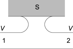
Figure 1: The NS junction connected to the superconductor (S) and two normal terminals $1$ and $2$.

The use standard scattering formalism for dynamics of charged quasiparticles. butt Fermionic operators for incoming and outgoing states, $\psi^{in}$ and $\psi^{out}$, respectively, are decomposed into modes, $\psi=\sum_{n}\psi_{n}c_{n}$, where $\psi_{n}$ is the normalized wavefunction of the mode and $c_{n}$ is the mode annihilation operator. The modes are related by unitary scattering matrix $s$, with $c_{n}^{out}=\sum_{m}s_{nm}c_{m}^{in}$.

We shall consider a junction between superconductor (ground) and two normal terminals at the same voltage $V$ in the way presented in Fig. 1. The reference point for energies is the middle of the superconducting gap. We include holes and Andreev reflection that converts electrons into holes and vice versa.and .

Electrons and holes move independently far from the superconductor. Accordingly, if the electron wavefunction is $\psi$, the corresponding one for holes is $\psi^{\ast}$. Hence, in the normal region, the scattering matrix for electrons, $s_{0}$ determines the one for holes, $s_{0}^{\ast}$.

The superconductor mixes, however, electrons and holes. The resulting scattering matrix can be written in the form

$$s=\left(\begin{array}[]{ll}s_{ee}&s_{eh}\\ s_{he}&s_{hh}\end{array}\right)\;.$$ (4)

In the normal region (no transitions between holes and electrons),

$$s_{N}=\left(\begin{array}[]{ll}s_{0}&0\\ 0&s_{0}^{\ast}\end{array}\right)\;.$$ (5)

On the other hand, the pure effect of superconductor – Andreev reflection, ignoring dynamics in the normal part, is

$$s_{A}=-i\left(\begin{array}[]{ll}0&e^{i\phi}\\ e^{-i\phi}&0\end{array}\right)\;,$$ (6)

where $\phi$ is the macroscopic phase of the superconductor, and we assume energies $E\ll\Delta$, where $2\Delta$ is the superconducting gap and is counted for the middle of the gap.

We decompose normal scattering matrix

$$s_{0}=\left(\begin{array}[]{ll}r&t\\ t^{T}&r^{\prime}\end{array}\right),$$ (7)

where the submatrix $r$ describes reflection for normal leads, $r^{\prime}$ – for the leads connected to the superconductor while $t$ and $t^{T}$ – transmission between normal and superconducting leads. Ignoring energy dependence and taking into account unitarity of $s_{0}$, we obtainbutt ; bee02 ; bee

$$s_{ee}=(1+rr^{\dagger})^{-1}(r+r^{T}+rr^{\dagger}(r-r^{T}))$$

$$s_{eh}=-ie^{i\phi}(1+rr^{\dagger})^{-1}(1-rr^{\dagger})$$

$$s_{he}=-ie^{-i\phi}(1+r^{\dagger}r)^{-1}(1-r^{\dagger}r)$$ (8)

$$s_{hh}=(1+r^{\dagger}r)^{-1}(r^{\ast}+r^{\dagger}+r^{\dagger}r(r^{\ast}-r^{\dagger}))\;.$$

Hence, the whole transport properties are described by $r$. We show in Appendix B that the ideal splitting is possible only at zero temperature.

IV Single mode terminals

Looking for ideal splitting, we restrict ourselves to the case of symmetric single mode terminals. so that $r$ depends only on two complex parameters,

$$r=\left(\begin{array}[]{ll}A&B\\ B&A\end{array}\right)\;.$$ (9)

In this case at zero temperature the ideal splitting yields the condition $A=0$, as we show in Appendix B. A similar matrix has been used in the previous calculations.tor00 However, the authors could not get ideal splitting since it is not possible in a three-mode $Y$ junction (see Appendix B).

For $A=0$, the matrix in the superconducting case has the simple form

$$s_{ee}=s_{hh}^{\ast}=\frac{2B}{1+|B|^{2}}\left(\begin{array}[]{rr}0&1\\ 1&0\end{array}\right),$$ (12)

$$s_{eh}=-s_{he}^{\ast}=-ie^{i\phi}\frac{1-|B|^{2}}{1+|B|^{2}}I.$$ (13)

The form of the scattering matrix $s$ given by (4) and (13) describes a process of either transmitting an electron to the neighboring terminal or reflecting it as a hole. We will use this simple interpretation later. In this case, using (1) and (A.4), we have

$$\bar{I}_{1}=\frac{4e^{2}V}{h}(1-|B|^{2})^{2}/(1+|B|^{2})^{2},$$ (14)

$$S_{11}=S_{12}=\frac{32e^{2}|eV|}{h}|B|^{2}(1-|B|^{2})^{2}/(1+|B|^{2})^{4}.$$

The magnitude of cross correlation is positive and maximal with respect to the CBS inequality in this case. In the limit $|B|\to 1$ we have $S_{12}\to 2|e\bar{I}_{1}|$. The maximum value of $S_{12}$ is $2e^{2}|eV|/h$ for $|B|^{2}=3-\sqrt{8}$. Importantly, cross noise vanishes in the normal case.

A transparent interpretation of our results can be given in terms of full counting statistics. We can use the event counting (A.5) for the scattering matrix (13), keeping in mind that incoming charge has to be subtracted while outgoing – added. Each electron incoming to the terminal $1$ can be either sent to the terminal $2$ or backscattered to $1$ as a hole. For electrons incoming to $2$, one has only to exchange the role of terminals. So, for each pair of electrons at $1$ and $2$, there are three possibilities, depicted in Fig. 2: (A) Both electrons are sent to the neighbor terminal with zero charge flow. (B) One of electrons is converted into a hole with charges $+e$ going out of the junction at each side. (C) Both electrons are converted into holes with charges $+2e$ at each side. The cross correlations are certainly positive.

In general, there could be other examples of ideal splitting, involving many-mode terminals. In principle, starting from the condition (B.2) one can find the constraints for $r$. However, the procedure becomes lengthy for large matrices.

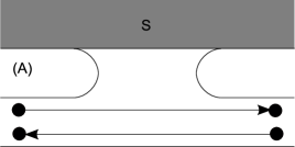
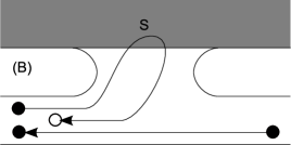
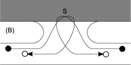
Figure 2: The three transport events at ideal splitting. Electrons are black and holes are white.(A) Both electrons pass. (B) One electron is converted into a hole. (C) Both electrons are converted.

V Average and shot noise

We shall derive the general formulas for the current and noise in the case of the junction described by reflection submatrix (9). We begin with the junction with all normal terminals, $1,2$ at voltage $V$, while the superconductor is replaced by ground. We assume that the scattering matrix is constant for energies in $[E_{F},E_{F}+eV]$ and $eV\ll E_{F}$. We consider only electrons (without holes). For each mode, there are two spin orientations. We shall use parameters $A$ and $B$ defined in (9), $C=|A|^{2}+|B|^{2}$, $D=1-C$, $w(x)=x\mathrm{cth}(x)$, $v=eV/k_{B}T$. Using Eqs. (A.4) and (1) we obtain

$$\bar{I}_{1}=\bar{I}_{2}=2e^{2}VD/h,\>S_{12}=S_{21}=-\frac{8e^{2}k_{B}T}{h}(|B|^{2}+$$

$$4(w(v/2)-1)\mathrm{Re}^{2}AB^{\ast}),$$ (15)

$$S_{11}=S_{22}=\frac{8e^{2}k_{B}T}{h}(D^{2}+|B|^{2}+w(v/2)CD).$$

In the case of NS junction two spin orientations will be replaced by two particle types - electrons and holes. The bias voltage $V$ is counted in reference to the middle of the superconductor gap, and it has the opposite effect on electrons and holes. We assume $|eV|,k_{B}T\ll\Delta$. We shall express mean current and noise by elements of matrices $r$ and $R=rr^{\ast}$. In our special case of the symmetric junction, we have $r=r^{T}$ and matrices $r$,$r^{\ast}$ and $R$ commute. From Eqs. (8) and (A.4) we have

$$\bar{I}_{1}=\bar{I}_{2}=\frac{4e^{2}V}{h}\left(\frac{(1-R)^{2}}{(1+R)^{2}}\right)_{11},$$

$$S_{11}=S_{22}=\frac{8k_{B}T}{h}(a+b(w(v)-1)),$$ (16)

$$S_{12}=S_{21}=\frac{8k_{B}T}{h}(c+d(w(v)-1)).$$

Here

$$a=1-4\left|\left(\frac{r}{1+R}\right)_{11}\right|^{2}+\left[\left(\frac{1-R}{1+R}\right)_{11}\right]^{2},$$

$$b=\left(\frac{4R}{(1+R)^{2}}\right)_{11}\left(\frac{(1-R)^{2}}{(1+R)^{2}}\right)_{11}\!\!\!\!+4\left|\left(\frac{r(1-R)}{(1+R)^{2}}\right)_{11}\right|^{2}\!\!,$$

$$c=\left[\left(\frac{1-R}{1+R}\right)_{12}\right]^{2}-4\left|\left(\frac{r}{1+R}\right)_{12}\right|^{2},$$ (17)

$$d=4\left|\left(\frac{r(1-R)}{(1+R)^{2}}\right)_{12}\right|^{2}-16\left[\left(\frac{R}{(1+R)^{2}}\right)_{12}\right]^{2}.$$

Denoting conductance by $G=\bar{I}_{1}/V$, the total noise has the form

$$S_{0}=4k_{B}TG(1+F(w(\tilde{v})-1)),$$ (18)

with $\tilde{v}=v/2$ and $\tilde{v}=v$ in the normal and superconducting case, respectively. The conductance $G$ and Fano factor $F\in[0,1]$ are different in both cases.

The values of cross correlation $S_{12}$ are always negative in the normal case, but they can be either negative or positive in the superconducting case. Interestingly, $S_{12}$ will be positive even at $V=0$ for positive $c$. This happens at $A=\exp(i\phi)(3-\sqrt{3})/2$ and $B=\exp(i\phi)(1-\sqrt{3})/2$ giving $c=+1/8$. This is possible for a $Y$ junction. However, this possibility is not mentioned in Ref. tor00, as only zero temperature case is there considered.

VI Resonance in the $X$-junction

Now, we would like to find a realistic geometry leading to the reflection submatrix (9) with $A=0$. We need at least two modes to be later connected to the superconductor, which is realized by the $X$-junction presented below.

Let us consider the following problem: how to find a potential that for a four-terminal junction and suitable geometry gives the scattering matrix without backscattering, i. e. with zero reflection amplitudes? This special case of scattering is often (mostly in three dimensions) referred to as Ramsauer-Townsend (RT) resonance.mott

We shall present such an example, starting from the usual two-dimensional Schrödinger equation

$$E_{F}\psi=-\frac{\hbar^{2}}{2m}\Delta\psi+V\psi$$ (19)

and the potential

$$V=\left\{\begin{array}[]{ll}+\infty&\mbox{ for }y\notin[0,W]\mbox{ or }y=W/2,x\notin[0,D]\\ 0&\mbox{ otherwise }\end{array}\right.$$ (20)

for the junction presented in Fig. 3. The symmetry helps to reduce the number of parameters describing the junction.

Figure 3: $X$-wire geometry with four modes: symmetric (s) and antisymmetric (a) modes are depicted. The upper, lower, and middle horizontal lines mark the infinite potential which pins down the wavefunction.

For the considered values of the Fermi energy $E_{F}=\hbar^{2}k_{F}^{2}/2m$ only single modes in the terminals and only two modes in the middle part of the junction are occupied, $k_{F}\in]2\pi/W,3\pi/W[$. It is convenient to introduce the wavenumbers $k_{1}=\sqrt{k_{F}^{2}-\pi^{2}/W^{2}}$ and $k_{2}=\sqrt{k_{F}^{2}-4\pi^{2}/W^{2}}$, which are real and positive in the considered range of $k_{F}$ values. Far from the junction the wavefunction has the form

$$\psi(x,y)=\sum_{j}(a_{j}\psi_{j}^{in}(x,y)+b_{j}\psi_{j}^{out}(x,y)).$$ (21)

Here $\psi_{j}^{in}=e^{i\epsilon_{j}k_{1}x}|\sin(2\pi y/W)|\theta_{j}(y)$ with $\epsilon_{1,3}=+1$, $\epsilon_{2,4}=-1$, $\theta_{1,2}(y)=\theta(y)\theta(W/2-y)$, $\theta_{3,4}(y)=\theta_{1,2}(W-y)$, and $\psi^{out}=(\psi^{in})^{\dagger}$. The Heaviside function $\theta$ reflects the vanishing of the wavefunction at the potential walls. The relation between amplitudes for ingoing and outgoing modes is given by

$$\left(\begin{array}[]{r}b_{1}\\ b_{2}\\ b_{3}\\ b_{4}\end{array}\right)=s_{0}\left(\begin{array}[]{r}a_{1}\\ a_{2}\\ a_{3}\\ a_{4}\end{array}\right),$$ (22)

which defines the scattering matrix $s$, satisfying unitarity condition $s^{\dagger}_{0}s_{0}=I$. Due to the geometric symmetry of the model, the scattering matrix can be expressed as

$$s_{0}=\frac{1}{2}\left(\begin{array}[]{rrrr}1&0&1&0\\ 0&1&0&1\\ 1&0&-1&0\\ 0&1&0&-1\end{array}\right)\left(\begin{array}[]{rr}s_{s}&0\\ 0&s_{a}\end{array}\right)\left(\begin{array}[]{rrrr}1&0&1&0\\ 0&1&0&1\\ 1&0&-1&0\\ 0&1&0&-1\end{array}\right).$$ (23)

Here $s_{s}$ and $s_{a}$ are scattering submatrices for symmetric ($1+3$, $2+4$) and antisymmetric modes ($1-3$, $2-4$), respectively. Since $\psi_{a}(y=W/2)=0$, the antisymmetric modes propagate unperturbed along the junction, which implies $s_{a}=I$.

The expected form of $s_{s}$ is

$$s_{s}=e^{i\theta}\left(\begin{array}[]{ll}i\alpha&\sqrt{1-\alpha^{2}}\\ \sqrt{1-\alpha^{2}}&i\alpha\end{array}\right),$$ (24)

where $\alpha\in[-1,1]$ and $\theta$ is a phase value.

Our final form matrix of the $s_{0}$ is then

$$\left(\begin{array}[]{cccc}A&B&A&C\\ B&A&C&A\\ A&C&A&B\\ C&A&B&A\end{array}\right)$$ (25)

with $2A=i\alpha\exp(i\theta)$, $2B=\sqrt{1-\alpha^{2}}\exp(i\theta)+1$ and $2C=\sqrt{1-\alpha^{2}}\exp(i\theta)-1$. It is clear that the requirement of absence backscattering implies $\alpha=0$.

An appropriately long $X$-junction can be seen as two $Y$-junctions depicted in Fig. 4(a) connected by a two mode channel, as shown in Fig. 4(b). We can express the corresponding values of $\alpha$ and $\theta$ by elements of the scattering matrix for the symmetric mode in the $Y$-junction

$$\left(\begin{array}[]{ll}a&b\\ b&c\end{array}\right),$$ (26)

where $c=-ba^{\ast}/b^{\ast}.$ From unitarity, we have $|a|^{2}+|b|^{2}=1$. The dependence of $a$ and $b$ on $k_{F}W$ can be determined numerically by properly matching propagating and evanescent modes, as explained in Appendix C.

Figure 4: (a) The $Y$-wire. (b)$X$-wire made of two $Y$-wires. Note that the symmetry allows the antisymmetric modes to propagate freely.

The parameters $\alpha$ and $\theta$ in the limit $D\gg W$ are given by

$$\alpha=\frac{\gamma}{\sqrt{1+\gamma^{2}}},\>e^{i\theta}=\frac{|b|^{4}e^{i(k_{1}-k_{2})D}\sqrt{1+\gamma^{2}}}{(b^{\ast})^{2}-b^{2}(a^{\ast})^{2}e^{2ik_{1}D}},$$ (27)

with

$$\gamma=2\mathrm{Im}\frac{ae^{-ik_{1}D}}{b^{2}}.$$ (28)

Now, the RT resonance ($\alpha=0$) is determined by

$$a(b^{\ast})^{2}=b^{2}a^{\ast}e^{2ik_{1}D},$$ (29)

and occurs at

$$D/W=(m\pi-\mathrm{arg}(b^{2}/a))/k_{1}W$$ (30)

for $m=1,2,3\dots$. Then

$$\theta=(k_{1}-k_{2})D+2\mathrm{arg}b.\>$$ (31)

We present a few lines of resonances for $k_{F}W/\pi\in[2,3]$ in Fig. 5. We stress that actual lines differ a little from Eq. (30) due to the approximation $D\gg W$. In general, in order to determine the exact positions of resonances, a residual contribution of evanescent modes in the middle part has to be taken into account.

The junction is connected to the superconductor as shown on Fig. 6. The predicted magnitudes of the cross shot noise (16) along the RT resonances given by (30) are presented in Fig. 7. Note that the noise magnitude reaches the maximum values given in Eq. (3).

Figure 5: Geometric ratios for resonances – absence of backscattering – given by Eq. (30).

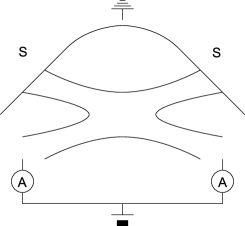
Figure 6: The geometry of an $X$ junction connected to a coherent superconductor (S).

Figure 7: The cross shot noise along the resonances given in Fig.5

Figure 8: The realistic junction with superconductor

VII Further modifications

The maximal cross shot noise shown in Fig. 7 requires not only ideal geometry and transparency but also tuning both $k_{F}W$ and $D/W$ according to (30). Moreover, non-zero temperature also usually decreases cross correlations.

Accordingly, we have considered the scattering problem for a more realistic device shown in Fig. 8, assuming an imperfect interface, taken into account within the Blonder, Tinkham and Klapwijk (BTK)btk model, varying the distance $L$ between the superconductor and the junction and/or allowing for a non-zero width $H$ of the internal gate between the terminals.

The scattering problem is solved by mode matching, taking into account not completely vanishing evanescent modes in the middle region. A single contact supports one mode for $k_{F}W\in]2\pi,4\pi[$. The transparency of non-ideal superconductor-normal metal interface in the BTK model reads $\Gamma=1/(1+Z^{2})$.

We present the results in Fig. 9 for $H=W/10$, $D=L=W$, $Z=0$, and $Z=0.5$.

Figure 9: The cross shot noise for ideal and non-ideal superconducting-normal interface for $D=L=W=10H$ as described in Fig. 8 for $Z=0$ and $0.5$. Note that in both cases $S_{12}$ can exceed maximal value $e\bar{I}_{1}$ for a single-mode superconductor.

The resonance seem to be wider and more robust for $k_{F}W<3\pi$ but large $L$ can turn it into several local maxima. However, $S_{12}$ still exceed $e\bar{I}_{1}$ for some range of parameters in contrast to previous results.tor00

It is clear that to get strong positive cross shot noise one should be able to tune the parameters of the junction since the noise is highly sensitive to changes. However, the general tendency is that the narrower the junction is, the more stable the noise magnitude is.

The presented $X$-junction may be difficult to realize experimentally. Therefore, we have analyzed also the case of $T$-junction with two modes going into the superconductor and single modes in normal terminals (Fig. 10). As shown in Fig. 11, the cross noise cannot reach the maximum $2e\bar{I}_{1}$ in such a geometry but still, for a certain range of parameters, it is larger than $e\bar{I}_{1}$. This large magnitude cannot be attained for any three-single-mode junction,tor00 in chaotic cavitySam00 or semiclassical regime. bro

Figure 10: The $T$-junction. Superconductor is attached from above to a normal quantum point contact

Figure 11: The cross shot noise of $T$-junction for some range of parameters. Note that the curve exceeds $1$ – the maximal value for all single modes

VIII Summary

We have proposed examples of X-junctions that exhibit, according to our theoretical results, large magnitudes of positive cross shot noise. Such a large magnitude could not be attained in the previously studied cases, such as three terminal devices with single modes in each leg or chaotic cavities containing many modes. The presented examples require separate connections to the phase coherent superconductor. One can, however, consider another example – simple Y or T junction, in which the leg connected to the superconductor contains at least two modes. The cross noise in this case can be also positive but not so large as in the X-junction. Nevertheless, in principle one should always be able to modify every four-mode junction in order to get maximal noise - ideal splitting of electrons. Hence, narrow wires are promising when searching for considerable positive cross correlations. Lastly, we would like to mention that some experiments to measure the cross shot noise in junctions discussed here are in preparation.

Appendix A

The long time properties of electronic transport are well described by full counting statistics, les ; naz with a generalization to the normal metal-superconductor interface. muz We consider the particle transfer statistics through a mesoscopic junction at given temperature $T$ and voltage bias $V$, without interactions. The junction has $m$ terminal/modes and a particle detector can be placed at each of them. During the measurement process a detector at the terminal/mode $\alpha$ registers the difference between numbers of particles outgoing from and ingoing to the junction $N_{\alpha}$. Here $\alpha$ denotes terminal, mode, spin and particle type (electron or hole). A set of registered numbers $\boldsymbol{N}=(N_{1},\dots,N_{m})$ occurs with a probability $p(\boldsymbol{N})$. Instead of probability, a very convenient tool to describe statistical properties of a probability distribution is the generating function.

$$e^{S(\boldsymbol{\lambda})}=\langle e^{i\boldsymbol{\lambda}\cdot\boldsymbol{N}}\rangle=\sum_{\boldsymbol{N}}p(\boldsymbol{N})e^{i\boldsymbol{\lambda}\cdot\boldsymbol{N}}.$$ (A.1)

Here $\boldsymbol{\lambda}=(\lambda_{1},\dots,\lambda_{m})$ is the vector of counting variables $\lambda_{\alpha}$. Using this form, it is straightforward to express averages and correlation functions as

$$\langle N_{\alpha}\rangle=-i\frac{\partial S}{\partial\lambda_{\alpha}},\>\langle\delta N_{\alpha}\delta N_{\beta}\rangle=-\frac{\partial^{2}S}{\partial\lambda_{\alpha}\partial\lambda_{\beta}}$$ (A.2)

for $\delta N_{\alpha}=N_{\alpha}-\langle N_{\alpha}\rangle$. On the other hand, the generating function at long times, $t_{0}\gg h/(|eV|+k_{B}T)$ is given by Levitov-Lesovik formulales

$$S=\frac{t_{0}}{h}\int dE\;\ln\mathrm{det}(1+n(s^{\dagger}e^{i\Lambda}se^{-i\Lambda}-1)).$$ (A.3)

Here $\Lambda$, $n$, $s$ and $s^{\dagger}$ are $m\times m$ matrices. The first two are diagonal with $\Lambda_{\alpha\alpha}=\lambda_{\alpha}$ and $n_{\alpha\alpha}=n_{\alpha}$. The latter describes occupation numbers, $n_{\alpha}=(1+\exp((E-q_{\alpha}V_{\alpha})/k_{B}T))^{-1}$ with $q_{\alpha}=-e$ for electrons and $+e$ for holes and $V_{\alpha}$ is the bias voltage. Exploiting the identity $\mathop{\rm tr}\ln=\ln\det$ the averages and correlations can be written as

$$\langle N_{\alpha}\rangle=\frac{t_{0}}{h}\int dE\;\mathop{\rm tr}P_{\alpha}(sns^{\dagger}-n),$$ (A.4)

$$\langle\delta N_{\alpha}\delta N_{\beta}\rangle=\frac{t_{0}}{h}\int dE\;\mathop{\rm tr}[sns^{\dagger}P_{\alpha}(1-sns^{\dagger})P_{\beta}$$

$$+n(1-n)(P_{\alpha}P_{\beta}-s^{\dagger}P_{\alpha}sP_{\beta}-s^{\dagger}P_{\beta}sP_{\alpha})]=$$

$$\frac{t_{0}}{h}\int dE\;\mathop{\rm tr}[n(s^{\dagger}P_{\alpha}s-P_{\alpha})(1-n)(s^{\dagger}P_{\beta}s-P_{\beta})]$$

where $P_{\alpha}$ denotes the projection on the mode $\alpha$ so that $P_{\alpha}$ commutes with $n$.

In this limit transport can be interpreted in terms of a series of elementary transport events. At time period $h/\Delta E$, detectors at each terminal can register an incoming particle, $\Delta N_{\alpha}=-1$, and/or an outgoing particle, $\Delta N_{\alpha}=+1$, or nothing. The probability value of the event that the set $I$ of ingoing particles is converted to the set $O$ of outgoing particles is given by

$$p(I\to O)=|\mathrm{det}\left(P_{I}sP_{O}\right)|^{2}\prod_{\alpha\in I}n_{\alpha}\prod_{\alpha\notin I}(1-n_{\alpha}),$$ (A.5)

where $P_{I}$ and $P_{O}$ denote the projections on the given set of modes/terminals. As the long time statistics can be interpreted classically, it also satisfies CBS inequality

$$\langle\delta Q_{A}\delta Q_{B}\rangle^{2}\leq\langle(\delta Q_{A})^{2}\rangle\langle(\delta Q_{B})^{2}\rangle$$ (A.6)

for $\delta Q_{X}=\sum_{\alpha\in X}q_{\alpha}\delta N_{\alpha}$ and arbitrary sets $A$ and $B$. To prove the inequality (A.6) it is enough to show that $\langle(\delta Q_{A}-z\delta Q_{B})^{2}\rangle\geq 0$ for $z=\langle\delta Q_{A}\delta Q_{B}\rangle/\langle(\delta Q_{B})^{2}\rangle$. Let us define $P_{z}=\sum_{\alpha\in A}q_{\alpha}P_{\alpha}-z\sum_{\alpha\in B}q_{\alpha}P_{\alpha}$. Then

$$\langle(\delta Q_{A}-z\delta Q_{B})^{2}\rangle=$$

$$\frac{t_{0}}{h}\int dE\;\mathop{\rm tr}[n(s^{\dagger}P_{z}s-P_{z})(1-n)(s^{\dagger}P_{z}s-P_{z})]$$

$$=\frac{t_{0}}{h}\int dE\;\mathop{\rm tr}K^{\dagger}K$$ (A.7)

for $K=\sqrt{n}(s^{\dagger}P_{z}s-P_{z})\sqrt{1-n}$ since $n^{\dagger}=n$. The trace of a Hermitian square is always positive, which completes the proof. Moreover, at zero temperature in the normal case, the noise is always sub-Poissonian if every terminal is either grounded or at the same voltage $V$,

$$\langle(\delta Q_{V})^{2}\rangle\leq|e\langle Q_{V}\rangle|$$ (A.8)

for $Q_{V}=\sum_{\alpha\in V}q_{\alpha}N_{\alpha}$ with summation over all terminals at $V$. To prove it, we use the fact that $n=\theta(-E)$ or $n=\theta(eV-E)$ for terminals at $0$ or $V$, respectively. Then, using (A.4) we get

$$\langle Q_{V}\rangle=\frac{t_{0}}{h}\int_{0}^{eV}edE\;\mathop{\rm tr}ss^{\dagger},$$ (A.9)

$$\langle(\delta Q_{V})^{2}\rangle=\frac{t_{0}}{h}\int_{0}^{eV}e^{2}dE\;\mathop{\rm tr}[ss^{\dagger}-(ss^{\dagger})^{2}]$$

We get (A.8) since $\mathop{\rm tr}(ss^{\dagger})^{2}\geq 0$. In the case of the ground replaced by the superconductor, the problem reduces to the normal case if NS surface is treated as a mirror, doubling the number of terminals for different quasiparticles. The total noise is

$$\langle(\delta Q)^{2}\rangle=\langle(\delta Q_{+})^{2}\rangle+\langle(\delta Q_{-})^{2}\rangle+2\langle\delta Q_{+}\delta Q_{-}\rangle$$ (A.10)

where $+$ and $-$ denote real and mirrored terminals, respectively. From CBS inequality (A.6) we get

$$\langle(\delta Q)^{2}\rangle\leq 2(\langle(\delta Q_{+})^{2}\rangle+\langle(\delta Q_{-})^{2}\rangle)$$ (A.11)

Using (A.8) we get

$$\langle(\delta Q)^{2}\rangle\leq 2(|e\langle Q_{+}\rangle|+|e\langle Q_{-}\rangle|)=2|e\langle Q\rangle|$$ (A.12)

because $\langle Q_{+}\rangle=-\langle Q_{-}\rangle$.

Appendix B

The CBS inequality (A.6) becomes equality only when $K=0$ in (A.7). For a finite temperature the ideal splitting gives the condition $s^{\dagger}P_{z=1}s=P_{z=1}$. The only possible scattering matrix in the basis $(1e,2e,1h,2h)$ has the block structure

$$s=\left(\begin{array}[]{rrrr}\ast&0&0&\ast\\ 0&\ast&\ast&0\\ 0&\ast&\ast&0\\ \ast&0&0&\ast\end{array}\right)$$ (B.1)

This means that the trace of $s_{eh}$ must vanish. However, from (8), it implies $\mathop{\rm tr}(2-T)T=0$ for $T=tt^{\dagger}=1-rr^{\dagger}$. For the fact that eigenvalues of $T$ lie between $0$ and $1$, the only possibility would be $t=0$ but this excludes superconductor completely and gives zero noise.

At zero temperature and finite voltage the condition $K=0$ has other solutions because $n_{e}\neq n_{h}$. The new requirement is

$$(s^{\dagger}P_{z=1}s)_{eh}=0$$ (B.2)

In our special case (9), using (8) we get the condition.

$$A^{\ast}(B^{2}-A^{2})=A.$$ (B.3)

The unitarity of $s_{0}$ imposes conditions $|A+B|\leq 1$ and $|A-B|\leq 1$. Together with (B.3) it implies either $A=0$ or $|A+B|=1=|A-B|$. The latter possibility again gives $t=0$ so we are left with the former one.

In the case of three mode junction we have

$$t=\left(\begin{array}[]{r}t_{1}\\ t_{2}\end{array}\right)$$ (B.4)

The unitarity condition yields $tt^{\dagger}$ proportional to identity matrix if $A=0$ in $r$. Hence, $|t_{1}|^{2}=|t_{2}|^{2}$ and $t_{1}^{\ast}t_{2}=0$ so $t_{1}=t_{2}=0$ and the superconductor decouples.

Appendix C

The symmetric wavefunction can be reduced to the interval $y\in[0,W/2]$ since

$$\psi(x,y)=\psi(x,W-y)$$ (C.1)

For $y\in[0,W/2]$ we have the following decomposition into $N+1\to\infty$ evanescent modes

$$\psi_{L}= \sin(2\pi y/W)(Ae^{ik_{2}x}+Be^{-ik_{2}x})+$$

$$\sum_{j=2}^{N+1}(-1)^{j}\sin(2j\pi y/W)E_{2j}e^{\kappa_{2j}x}$$

$$\psi_{R}= \sin(\pi y/W)Ce^{ik_{1}x}+$$

$$\sum_{l=1}^{N}(-1)^{l}\sin((2l+1)\pi y/W)E_{2l+1}e^{-\kappa_{2l+1}x}$$

where

$$\kappa_{n}W=\sqrt{n^{2}\pi^{2}-(k_{F}W)^{2}},\>n=3,4,\dots$$ (C.3)

The boundary conditions (integration with $\chi_{2j}(y)$, $y\in[0,W/2]$) are

$$\int_{0}^{W/2}dy\;\sin\left(\frac{2j\pi y}{W}\right)(\psi_{L}(0,y)-\psi_{R}(0,y))=0$$

$$\int_{0}^{W/2}dy\>\sin\left(\frac{2j\pi y}{W}\right)\partial_{x}(\psi_{L}(0,y)-\psi_{R}(0,y))=0$$

We make use of trigonometric identities and integrals

$$\int_{0}^{W/2}dy\>\sin^{2}(2j\pi y/W)=W/4$$ (C.4)

$$\int_{0}^{W/2}dy\>\sin(2j\pi y/W)\sin((2l+1)\pi y/W)=$$

$$\frac{W}{2\pi}(-1)^{l+j}\frac{4j}{(2l+1)^{2}-4j^{2}}$$

We get the following equations for $A=1$, $B$, $C$, $E_{3}$, $E_{4}$,…$E_{2N+2}$ and $j=2,\dots N+1$,

$$A+B=\frac{8}{3\pi}C-\sum_{l=1}^{N}\frac{8}{\pi}\frac{E_{2l+1}}{(2l+1)^{2}-4}$$

$$E_{2j}=\frac{8j}{\pi}\frac{C}{1-4j^{2}}+\sum_{l=1}^{N}\frac{8j}{\pi}\frac{E_{2l+1}}{(2l+1)^{2}-4j^{2}},$$

$$ik_{2}(A-B)=\frac{8}{3\pi}ik_{1}C+\sum_{l=1}^{N}\frac{8}{\pi}\frac{\kappa_{2l+1}E_{2l+1}}{(2l+1)^{2}-4}$$ (C.5)

$$\kappa_{2j}E_{2j}=\frac{8j}{\pi}\frac{ik_{1}C}{1-4j^{2}}-\sum_{l=1}^{N}\frac{8j}{\pi}\frac{\kappa_{2l+1}E_{2l+1}}{(2l+1)^{2}-4j^{2}},$$

The elements of the matrix (26) are given by

$$a=\frac{B}{A},\>b=\sqrt{\frac{k_{1}}{k_{2}}}\frac{C}{A}.$$ (C.6)

Note that for finite $N$ the unitarity condition $|a|^{2}+|b|^{2}=1$ may be not exactly satisfied.

References

- (1) For a review, see Ya. M. Blanter, M. Büttiker, Phys. Rep. 336, 1 (2000).
- (2) R. Hanbury Brown and R.Q. Twiss, Nature 177, 27 (1956).
- (3) M. Büttiker, Phys. Rev. B 46, 12485 (1992).
- (4) M. Hennyet al. Science 284, 296 (1999); W.D. Oliver et al. Science 284, 299 (1990); S. Oberholzer et al., Physica E 6, 314 (2000).
- (5) M.P. Anantram and S. Datta, Phys. Rev. B 53, 16390 (1996).
- (6) C. W. J. Beenakker, Phys. Rev. B 46, 12841 (1992).
- (7) J. Torrés and Th. Martin, Eur. Phys. J. B 12, 319 (1999).
- (8) T. Martin, Phys. Lett. A 220, 137 (1996).
- (9) M. Schechter, Y. Imry, and Y. Levinson, Phys. Rev. B 64, 224513 (2001).
- (10) F. Taddei and R. Fazio, Phys. Rev. B 65, 134522 (2002).
- (11) G. Bignon et al., Europhys. Lett. 67, 110(2004).
- (12) S. Duhot, F. Lefloch, and M. Houzet, Phys. Rev. Lett. 102, 086804 (2009).
- (13) P. Samuelsson and M. Büttiker, Phys. Rev. Lett. 89 (2002) 046601.
- (14) B.-R.Choi et al., Phys. Rev. B 72, 024501 (2005).
- (15) J. Torres, T. Martin, G.B. Lesovik, Phys. Rev. B 63, 134517 (2001).
- (16) J. Nilsson, A.R. Akhmerov, and C.W.J. Beenakker, Phys. Rev. Lett. 101, 120403 (2008)
- (17) G.B. Lesovik, T. Martin, G. Blatter, Eur. J. Phys. B 24, 287 (2001).
- (18) K.V. Bayandin, G.B. Lesovik, T. Martin, Phys. Rev. B 74, 085326 (2006).
- (19) V. Bouchiat et al., Nanotechnology 14 77 (2003).
- (20) D. Sanchez et al., Phys. Rev. B 68, 214501 (2003).
- (21) N. F. Mott and H. S. W. Massey, The Theory of Atomic Collisions, Oxford University Press, London, 1965.
- (22) G. Grabecki et al., Phys. Rev. B 72, 125332 (2005).
- (23) A. F. Andreev, Zh. Eksp. Teor. Fiz. 46, 1823 (1964) [Sov. Phys. JETP 19, 1228 (1964)].
- (24) C. W. J. Beenakker, Rev. Mod. Phys. 69, 731 (1997), chapter 4.
- (25) L.S. Levitov and G.B. Lesovik, JETP Lett. 58, 230 (1993); L.S. Levitov, H.W. Lee, and G.B. Lesovik, J. Math. Phys. 37, 4345 (1996).
- (26) W. Belzig and Y.V. Nazarov, Phys. Rev. Lett. 87, 197006 (2001); M. Kindermann and Y.V. Nazarov, in: Quantum Noise in Mesocopic Physics, Y.V. Nararow, ed., (Kluwer, Dordrecht, 2003).
- (27) B. A. Muzykantskii and D. E. Khmelnitskii, Phys. Rev. B 50, 3982 (1994).
- (28) J.P. Morten et al., Phys. Rev. B 74, 214510 (2006); 78, 224515 (2008); Europhys. Lett. 81, 40002 (2008).
- (29) G.E. Blonder, M. Tinkham, and T.M. Klapwijk, Phys. Rev. B 25, 4515 (1982).
- (30) J. Börlin, W. Belzig, and C. Bruder, Phys. Rev. Lett. 88 197001 (2002).