Light scalar mesons: comments on their behavior in the $1/N_{c}$ expansion near $N_{c}=3$ versus the $N_{c}\rightarrow\infty$ limit

Abstract

We briefly review how light meson resonances are described within one and two-loop Unitarized Chiral Perturbation Theory amplitudes and how, close to $N_{c}=3$, light vectors follow the $N_{c}$ behavior of $q\bar{q}$ mesons whereas light scalars do not. This supports the hypothesis that the lightest scalar is not predominantly a $q\bar{q}$ meson, although a subdominant $q\bar{q}$ component is suggested around 1 GeV at somewhat larger $N_{c}$. In contrast, when $N_{c}$ is very far from 3, like in the $N_{c}\rightarrow\infty$ limit, we explain again in detail why unitarization is not, a priori, reliable nor robust and why this limit should not be used to drag any conclusions about the dominant nature of physical light scalar mesons.

12.39.Mk, 11.15.Pg, 12.39.Fe, 13.75.Lb

1 Introduction

The $1/N_{c}$ expansion [1] is the only analytic expansion of QCD in the whole energy region, that provides a definition of $\bar{q}q$ bound states, whose masses and widths behave as $O(1)$ and $O(1/N_{c})$, respectively. Light mesons are also described within Chiral Perturbation Theory (ChPT)[2], which is the QCD low energy effective theory, built as the most general effective lagrangian compatible with all QCD symmetries, involving the pseudo Nambu-Goldstone Bosons of the QCD spontaneous chiral symmetry breaking. Meson-meson scattering amplitudes become an expansion in momenta and masses, generically denoted $p$, over a scale $\Lambda_{\chi}\sim 4\pi f_{\pi}\simeq 1$ GeV. At each order, the ChPT Lagrangian contains all terms compatible with QCD symmetries, multiplied by Low Energy Constants (LECs), that encode the QCD dynamics and renormalize divergences order by order.

The correct QCD leading order $1/N_{c}$ behavior of $f_{\pi}$, the pseudo Nambu-Goldstone boson masses and the LECs, is well known and ChPT amplitudes have no cutoffs or subtraction constants where spurious $N_{c}$ dependences could hide. Note that, in order to apply the $1/N_{c}$ expansion, the renormalization scale $\mu$ has been chosen between $\mu=$ 0.5 and 1 GeV, following [2]. (Also, in Fig. 1 we show that outside this band the generated vector mesons will start deviating from their well established $\bar{q}q$ behavior).

Resonances are not present in the ChPT lagrangian but can be described using ChPT as input in a dispersion relation [3]. The main idea is that partial waves, $t$, of definite isospin and angular momentum satisfy an elastic unitarity condition: ${\mbox{Im}\,}1/t=-\sigma,$ while the ChPT expansion $t\simeq t_{2}+t_{4}+\cdots$, $t_{k}=O(p^{k})$, satisfies it only perturbatively: ${\mbox{Im}\,}t_{2}=0,{\mbox{Im}\,}t_{4}=\sigma|t_{2}|^{2},\cdots$.

Since $G=t_{2}^{2}/t$ has a right cut ($RC$) a left cut ($LC$), and possible pole contributions ($PC$), we can write a dispersion relation as follows

$$G(s)=G(0)+G^{\prime}(0)s+\tfrac{1}{2}G^{\prime\prime}(0)s^{2}+\frac{s^{3}}{\pi}\int_{RC}ds^{\prime}\frac{{\mbox{Im}\,}G(s^{\prime})}{s^{\prime 3}(s^{\prime}-s)}+LC(G)+PC.$$ (1)

In the elastic approximation, unitarity allows us to evaluate exactly ${\mbox{Im}\,}G=-\sigma t_{2}^{2}=-{\mbox{Im}\,}t_{4}$ on the $RC$. The subtraction constants can be approximated with ChPT since they involve amplitudes evaluated at $s=0$, $G(0)\simeq t_{2}(0)-t_{4}(0),\cdots$. These three subtractions imply that $LC$ is dominated by its low energy part, and well estimated by ChPT as $LC(G)\simeq LC(-t_{4})$. $PC$ counts as $O(p^{6})$ and only gives sizable contributions much below threshold in scalar waves [4], thus we neglect it here for simplicity. All in all, one finds the IAM formula [3]:

$$t(s)\simeq\frac{t_{2}^{2}(s)}{t_{2}(s)-t_{4}(s)}\,.$$ (2)

Remarkably, this simple equation ensures elastic unitarity, matches ChPT at low energies, describes fairly well data up to somewhat less than 1 GeV, and generates the $\rho$, $K^{*}$, $\sigma$ and $\kappa$ resonances as poles on the second Riemann sheet, with ChPT parameters rather similar to those from standard ChPT. The IAM can be easily extended to higher orders or – without a dispersive justification yet – generalized within a coupled channel formalism [5, 6], generating also the $a_{0}(980)$, $f_{0}(980)$ and the octet $\phi$.

By scaling with $N_{c}$ the ChPT parameters in the IAM, we can determine the $N_{c}$ dependence of the resonances masses and widths [7, 8], defined from the pole position as $\sqrt{s_{pole}}=M-i\Gamma$, and compare it with the $\bar{q}q$ scaling to determine if the resonance is predominantly of a $\bar{q}q$ nature.

However, a priori, one should be careful not to take $N_{c}$ too large, and in particular to avoid the $N_{c}\to\infty$ limit, because it is a weakly interacting limit. As shown above, the IAM relies on the fact that the exact elastic $RC$ contribution dominates the dispersion relation. Since the IAM describes the data and the resonances, within, say 10 to 20% errors, this means that at $N_{c}=3$ the other contributions are not approximated badly. But meson loops, responsible for the $RC$, scale as $3/N_{c}$ whereas the inaccuracies due to the approximations scale partly as $O(1)$. Thus, we can estimate that those 10 to 20% errors at $N_{c}=3$ may become 100% errors at, say $N_{c}\sim 30$ or $N_{c}\sim 15$, respectively. Hence we have never shown results [7, 8] beyond $N_{c}=30$, and even beyond $N_{c}\sim 15$ they should be interpreted with care.

Of course, there could be special cases in which the IAM could still work for very large $N_{c}$, as it is has been shown for the vector channel for QCD [9]. But that is not the case for the scalar channel, which, if used for too large $N_{c}$ may lead to inconsistencies [9] for some values of the LECS.

2 $N_{c}$ scaling of resonances

The $N_{c}$ scaling of IAM resonances was studied to one-loop in coupled channels in [7] and to two-loops in the elastic case in [8]. Thus, Fig.1 shows the behavior of the $\rho$, $K^{*}$ and $\sigma$ masses and widths found in [7]. The $\rho$ and $K^{*}$ neatly follow the expected behavior for a $\bar{q}q$ state: $M\sim 1$, $\Gamma\sim 1/N_{c}$. The bands cover the uncertainty in $\mu\sim 0.5-1$ GeV where to scale the LECs with $N_{c}$. Note also in Fig.1(Top-right) that, for that set of LECS, outside this $\mu$ range the $\rho$ meson starts deviating from a a $\bar{q}q$ behavior. Something similar occurs to the $K^{*}(892)$. Consequently, we cannot apply the $N_{c}$ scaling at an arbitrary $\mu$ value, if the well established $\rho$ and $K^{*}$ $\bar{q}q$ nature is to be reproduced.

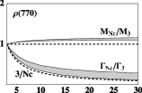
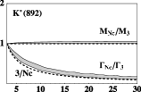
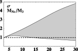
Figure 1: Top: $N_{c}$ behavior of the $\rho$ and $K^{*}$ mass and width (left and center). Right: Different $\rho$ pole trajectories for different values of $\mu$, note that for $\mu=1.2$ GeV the $\rho$ pole goes away the real axis. Bottom: $N_{c}$ behavior of the $\sigma$ mass and width (left and center). Right: Different $\sigma$ pole trajectories for different $\mu$ values.

In contrast, the $\sigma$ shows a different behavior from that of a pure $\bar{q}q$: near $N_{c}$=3 both its mass and width grow with $N_{c}$, i.e. its pole moves away from the real axis. Of course, far from $N_{c}=3$, and for some choices of LECs and $\mu$, the sigma pole might turn back to the real axis [8, 9, 11], as seen in Fig.1 (Bottom-right). But, as commented above, the IAM is less reliable for large $N_{c}$, and even if we trust this behavior it only suggests that there might be a subdominant $\bar{q}q$ component [8]. In addition, we have to make sure that the LECs used fit data and reproduce the $\bar{q}q$ behavior for the vectors.

Since loop terms are important in determining the scalar pole position, but are $1/N_{c}$ suppressed compared to tree level terms with LECs, it is relevant to check the $O(p^{4})$ results with an $O(p^{6})$ IAM calculation. This was done within $SU(2)$ ChPT in [8]. We defined a $\chi^{2}$-like function to measure how close a resonance is from a $\bar{q}q$ $N_{c}$ behavior. First, we used that $\chi^{2}$-like function at $O(p^{4})$ to show that it is not possible for the $\sigma$ to behave predominantly as a $\bar{q}q$ while describing simultaneously the data and the $\rho$ $\bar{q}q$ behavior, thus confirming the robustness of the conclusions for $N_{c}$ close to 3. Next, we obtained a $O(p^{6})$ data fit – where the $\rho$ $\bar{q}q$ behavior was imposed – whose $N_{c}$ behavior for the $\rho$ and $\sigma$ mass and width is shown in Fig.2. Note that both $M_{\sigma}$ and $\Gamma_{\sigma}$ grow with $N_{c}$, near $N_{c}=3$ confirming the $O(p^{4})$ result of a non $\bar{q}q$ dominant component. However, as $N_{c}$ grows further, between $N_{c}\sim 8$ and $N_{c}\sim 15$, where we still trust the IAM results, $M_{\sigma}$ becomes constant and $\Gamma_{\sigma}$ starts decreasing. This may hint to a subdominant $\bar{q}q$ component, arising as loop diagrams become suppressed as $N_{c}$ grows. Finally, we checked how big this $\sigma$ $\bar{q}q$ component can be made, by forcing the $\sigma$ to behave as a $\bar{q}q$ using the above mentioned $\chi^{2}$-like measure. We found that in the best case, this subdominant $\bar{q}q$ component could become dominant around $N_{c}>6$, at best, but always with an $N_{c}\to\infty$ mass above roughly 1 GeV instead of its physical $\sim 450$ MeV value.

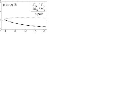
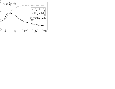
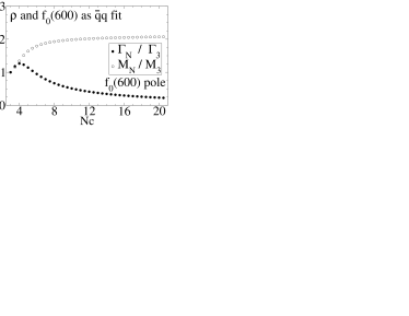
Figure 2: Right and center: $N_{c}$ behavior of the $\rho$ and $\sigma$ pole at $O(p^{6})$ with the “$\rho$ as $\bar{q}q$ fit”. Center: Sigma behavior with $N_{c}$ at $O(p^{6})$ with the “$\sigma$ as $\bar{q}q$ fit”.

3 Discussion and conclusions

We have seen that, within ChPT unitarized with the IAM, the $N_{c}$ behavior of $\bar{q}q$ states is clearly identified whereas scalar mesons behave differently near $N_{c}=3$. Here we want to emphasize again [12], what can and what cannot be concluded from this behavior and clarify some frequent questions and doubts raised in this meeting, private discusions and the literature:

• The dominant component of the $\sigma$ and $\kappa$ in meson-meson scattering does not behave as a $\bar{q}q$. Why “dominant”? Because, most likely, scalars are a mixture of different kind of states. If the $\bar{q}q$ was dominant, they would behave as the $\rho$ or the $K^{*}$ in Fig.1. But a smaller fraction of $\bar{q}q$ cannot be excluded. Actually, it is somewhat favored in our $O(p^{6})$ analysis [8].

• Two meson and some tetraquark states[10] have a consistent “qualitative” behavior, i.e., both disappear in the meson-meson scattering continuum as $N_{c}$ increases. Our results are not able yet to establish the nature of that dominant component. The most we could state is that the behavior of two-meson states or some tetraquarks might be qualitatively consistent.

The $N_{c}\rightarrow\infty$ limit has been studied in [11, 9]. Apart from its mathematical interest, it could have some physical relevance if the data and the large $N_{c}$ uncertainty on the choice of scale were more accurate. Nevertheless:

• As commented above, a priori the IAM is not reliable in the $N_{c}\rightarrow\infty$ limit, since it corresponds to a weakly interacting theory, where exact unitarity becomes less relevant in confront of other approximations made in the IAM derivation. It has been shown [9] that it might work well in that limit in the vector channel of QCD but not in the scalar channel.

• Another reason to limit ourselves to $N_{c}$ not too far from 3 is that in our calculations we have not included the $\eta^{\prime}(980)$, whose mass is related to the $U_{A}(1)$ anomaly and scales as $\sqrt{3/N_{c}}$. Nevertheless, if in our calculations we keep $N_{c}<30$, its mass would be $>310\,$MeV and thus pions are still the only relevant degrees of freedom for the scalar channel in the $\sigma$ region.

• Contrary to the leading $1/N_{c}$ behavior in the vicinity of $N_{c}=3$, the $N_{c}\rightarrow\infty$ limit does not give information on the “dominant component” of light scalars. The reason was commented above: In contrast to $\bar{q}q$ states, that become bound, two-meson and some tetraquark states dissolve in the continuum as $N_{c}\rightarrow\infty$. Thus, even if we started with an infinitesimal $\bar{q}q$ component in a resonance, for a sufficiently large $N_{c}$ it may become dominant, and beyond that $N_{c}$ the associated pole would behave as a $\bar{q}q$ state although the original state only had an infinitesimal admixture of $\bar{q}q$. Also, since the mixings of different components could change with $N_{c}$, a too large $N_{c}$ could alter significantly the original mixings.

Actually, this is what happens for the one-loop IAM $\sigma$ resonance for $N_{c}\to\infty$, but it does not necessarily mean that the “correct interpretation… is that the $\sigma$ pole is a conventional $\bar{q}q$ meson environed by heavy pion clouds” [11]. That the scalars are not conventional, is simply seen by comparing them in Figs.1 and 2 with the “conventional” $\rho$ and $K^{*}$ in those very same figures. A large two-meson component is consistent, but the $N_{c}\rightarrow\infty$ of the one-loop unitarized ChPT pole in the scalar channel limit is not unique [11, 9] given the uncertainty in the chiral parameters. Moreover, for some LECS the scalar channel one-loop IAM in the $N_{c}\rightarrow\infty$ limit can lead to phenomenological inconsistencies [9] since poles can even move to negative mass square (weird), to infinity or to a positive mass square. That is one of the reasons why in the figures here and in [7, 8] we only plot up to $N_{c}=30$, but not 100, or a million. Hence, robust conclusions on the dominant light scalar component, can be obtained not too far from real life, say $N_{c}<15$ or 30, for a $\mu$ choice between roughly $0.5$ and 1 GeV, that simultaneously ensures the $\bar{q}q$ dependence for the $\rho$ and $K^{*}$ mesons. Note, however, that under these same conditions the two-loop IAM still finds a dominant non-$\bar{q}q$ component, but, in addition, a hint of a $\bar{q}q$ subdominant component, which is not conventional in the sense that it appears at a much higher mass than the physical $\sigma$. This may support the existence of a second $\bar{q}q$ scalar octet above 1 GeV [13].

In summary, the dominant component of light scalars as generated from unitarized one loop ChPT scattering amplitudes does not behave as a $\bar{q}q$ state as $N_{c}$ increases not far from $N_{c}=3$. When using the two loop IAM result in SU(2), below $N_{c}\sim\,$15 or 30, there is a hint of a subdominant $\bar{q}q$ component, but arising at roughly twice the mass of the physical $\sigma$.

References

- [1] G. ’t Hooft, Nucl. Phys. B 72 (1974) 461. E. Witten, Ann. Phys. 128 (1980) 363.
- [2] J. Gasser and H. Leutwyler, Ann. Phys.158,142(1984). Nucl.Phys.B250(1985)465.
- [3] T. N. Truong, Phys. Rev. Lett. 61 (1988) 2526. Phys. Rev. Lett. 67, (1991) 2260; A. Dobado, M.J.Herrero and T.N. Truong, Phys. Lett. B235 (1990) 134. A. Dobado and J. R. Pelaez, Phys. Rev. D 47 (1993) 4883. Phys. Rev. D 56 (1997) 3057.
- [4] A. Gomez Nicola, J. R. Pelaez and G. Rios, Phys. Rev. D 77, 056006 (2008)
- [5] A. Gomez Nicola and J. R. Pelaez, Phys. Rev. D 65, 054009 (2002) J. R. Pelaez, Mod. Phys. Lett. A 19, 2879 (2004)
- [6] J. A. Oller, E. Oset and J. R. Pelaez, Phys. Rev. Lett. 80 (1998) 3452; Phys. Rev. D 59 (1999) 074001 J. A. Oller and E. Oset, Nucl. Phys. A 620, 438 (1997) [Erratum-ibid. A 652, 407 (1999)] and Phys. Rev. D 62 (2000) 114017. F. Guerrero and J. A. Oller, Nucl. Phys. B 537, 459 (1999) [Erratum-ibid. B 602, 641 (2001)]
- [7] J. R. Pelaez, Phys. Rev. Lett. 92, 102001 (2004).
- [8] J. R. Pelaez and G. Rios, Phys. Rev. Lett. 97, 242002 (2006)
- [9] J. Nieves and E. R. Arriola, arXiv:0904.4344 [hep-ph].
- [10] R. L. Jaffe, Proc. of the Intl. Symposium on Lepton and Photon Interactions at High Energies. Physikalisches Institut, Univ. of Bonn (1981). ISBN: 3-9800625-0-3.
- [11] Z. X. Sun, et al.Z. X. Sun, et al.[arXiv:hep-ph/0503195].
- [12] J. R. Pelaez, arXiv:hep-ph/0509284. Proceedings of the 11th International Conference on Elastic and Diffractive Scattering, Blois, France, 15-20 May 2005.
- [13] E. Van Beveren, et al. Z. Phys. C 30, 615 (1986) and hep-ph/0606022. E. van Beveren and G. Rupp, Eur. Phys. J. C 22 (2001) 493, J. A. Oller and E. Oset, Phys. Rev. D 60 (1999) 074023. F. E. Close and N. A. Tornqvist, J. Phys. G 28, R249 (2002).