Equivalence between the mobility edge of electronic transport on disorder-less networks and the onset of chaos via intermittency in deterministic maps

Abstract

We exhibit a remarkable equivalence between the dynamics of an intermittent nonlinear map and the electronic transport properties (obtained via the scattering matrix) of a crystal defined on a double Cayley tree. This strict analogy reveals in detail the nature of the mobility edge normally studied near (not at) the metal-insulator transition in electronic systems. We provide an analytical expression for the conductance as function of system size that at the transition obeys a $q$-exponential form. This manifests as power-law decay or few and far between large spike oscillations according to different kinds of boundary conditions.

Occasionally the detection of a deep running analogy between two apparently different physical problems allows for the determination of elusive quantities and understanding of difficult issues. Here we present a relationship between intermittency and electronic transport. This development brings together fields of research in nonlinear dynamics and condensed matter physics. Specifically, the dynamics at the onset of chaos appears associated to the critical conductance at the mobility edge of regular self-similar networks mobility .

Recently, the dynamics at the transitions to chaos that occurs along the three known universal routes from regular to irregular behavior (in low-dimensional nonlinear maps) has been analyzed with a good deal of detail Baldovin2002 -Robledo2008 . This effort has helped establish the nature of the statistical-mechanical structure obeyed by the dynamics associated to nonmixing and nonergodic attractors Robledo2008 . On the other hand, there are known connections between nonlinear dynamical systems and electronic transport properties. For example, there are models for transport in incommensurate systems, where Schrödinger equations with quasiperiodic potentials Harper1955 are equivalent to nonlinear maps with a quasiperiodic route to chaos, and where the divergence of the localization length translates into the vanishing of the ordinary Lyapunov coefficient Ketoja1997 .

At the tangent bifurcation Baldovin2002 , the focal point of the intermittency route to chaos, an uncommon but welcome simplicity has led to analytical results in closed form for the dynamics at vanishing Lyapunov exponent Baldovin2002 . Here we make full use of this circumstance showing that transport in a model network, a double Cayley tree, resolved by means of the scattering matrix, is given by the properties of a one-dimensional nonlinear map. The model, in this study, does not contain disorder; nevertheless it displays a transition between localized and extended states. The translation of the map dynamical features into electronic transport terms provides not only the description of the two different conducting phases but, we believe, offers for the first time a rigorous account of the conductance at the mobility edge. A type of localization length in the incipient insulator mirrors the departure from exponential sensitivity to initial conditions at the transition to chaos.

We recap briefly the usefulness of Cayley tree networks in the study of electronic transport properties in the presence, and absence, of disorder. A single Cayley tree spans over a space of infinite dimensionality Straley and transport on it exhibits a metal-insulator transition as a function of disorder abouchacra . A scattering approach was applied in Ref. ShapiroPRL1983 for off-diagonal disorder and shown that the metal-insulator transition occurs for connectivity $K\geq 2$ ($K+1$ is the coordination number). A single Cayley tree is a first approximation to an ordinary regular lattice abouchacra , but, as shown below, a double Cayley tree (two single Cayley trees joined conformally as in Fig. 1) is a much better approximation (see also Zekri ). In Ref. Avishai1992 is shown that the conducting band of a disorder-less double Cayley tree contracts and disappears as $K$ increases. In Ref. Horvat the dynamic behaviour of a chain of scatterers was analyzed in the absence and presence of disorder; while the localization transition for different types of complex networks, including the double Cayley tree, was studied in Ref. Sade via spectral statistics. Finally, the double Cayley tree problem is relevant for transport in chaotic cavities with broken mirror symmetry GMMB . Here we show that the electronic structure for $K=2$ can be determined by reducing the scattering matrix to a nonlinear map. This development facilitates the band description of the conductance as a function of energy including the location of the mobility edge.

Figure 1: A double Cayley tree of conectivity $K=2$ and lattice constan $a$. Each bond is a perfect one dimensional conductor.

Here we consider electronic transport in the double Cayley tree (see Fig. 1). We refer only to the ordered, crystal-like, system and reduce its associated scattering matrix to a nonlinear map. The number of times the trees are ramified, starting from perfect join, is the generation $n$ that quantifies the size of the system. Also, for brevity, we will fix the tree connectivity to $K=2$ where one lead, we call it the incoming lead, is divided into two leads at a given node. The leads are assumed to be equivalent to one dimensional perfect wires with length equal to the lattice constant $a$ and are independent of $n$. Hence, each node is described by the same $3\times 3$ scattering matrix for which we assume the model Buettiker1984

$$S_{\text{node}}=\left[\begin{array}[]{ccc}-(\alpha+\beta)&\sqrt{\epsilon}&\sqrt{\epsilon}\\ \sqrt{\epsilon}&\alpha&\beta\\ \sqrt{\epsilon}&\beta&\alpha\end{array}\right],$$ (1)

where $\epsilon$, a real number in the interval $0\leq\epsilon\leq\frac{1}{2}$, is the transmission probability (or coupling) from the incoming lead to the others, and viceversa. The reflection amplitude to the incoming lead is $-(\alpha+\beta)$, with $\alpha=-(1-\sqrt{1-2\epsilon})/2$ and $\beta=(1+\sqrt{1-2\epsilon})/2$. When incidence is only on one of the other two leads $\alpha$ is the reflection amplitude to the same lead and $\beta$ the transmission amplitude to the other lead.

The scattering matrix of the system is $2\times 2$ and satisfies a recursive relation. If we denote by $S_{n}$ the scattering matrix at generation $n$, the combination rule for scattering matrices allows $S_{n}$ to be written in terms of the scattering matrix at a previous generation $n-1$,

$$S_{n}=\frac{-1}{e^{-2ika}\openone-\sqrt{1-2\epsilon}S_{n-1}}(\sqrt{1-2\epsilon}\,e^{-2ika}\openone-S_{n-1}),$$ (2)

with $\openone$ the $2\times 2$ identity matrix. The scattering matrix at a generation $n$ can be obtained iteratively starting from that for the perfect union in the middle of our double Cayley tree: $S_{0}=\sigma_{x}$, where $\sigma_{x}$ is a Pauli matrix.

Firstly, it can be seen that $S_{n}$ is a unitary matrix, which is the condition of flux conservation. Then, time reversal invariance restricts $S_{n}$ to be a symmetric matrix. Finally, the additional lattice spatial reflection symmetry implies that $S_{n}$ has the form GMMB

$$S_{n}=\left(\begin{array}[]{cc}r_{n}&t_{n}\\ t_{n}&r_{n}\end{array}\right),$$ (3)

where $r_{n}$ and $t_{n}$ are the reflection and transmission amplitudes. With this structure $S_{n}$ is diagonalized by a $\pi/4$-rotation GMMB ; that is

$$\left(\begin{array}[]{cc}e^{i\theta_{n}}&0\\ 0&e^{i\theta_{n}^{\prime}}\end{array}\right)=\frac{1}{\sqrt{2}}\left(\begin{array}[]{rc}1&1\\ -1&1\end{array}\right)S_{n}\frac{1}{\sqrt{2}}\left(\begin{array}[]{cr}1&-1\\ 1&1\end{array}\right).$$ (4)

Here, $\theta_{n}$ and $\theta_{n}^{\prime}$ are the eigenphases that satisfy $e^{i\theta_{n}}=r_{n}+t_{n}$ and $e^{i\theta_{n}^{\prime}}=r_{n}-t_{n}$. In terms of the eigenphases the transmission amplitude is given by $t_{n}=\frac{1}{2}(e^{i\theta_{n}}-e^{i\theta_{n}^{\prime}})$. Morever, the dimensionless conductance (i.e. in units of $2e^{2}/h$) depends on the eigenphases through Landauer’s formula as Landauer ; IBM ,

$$g_{n}=|t_{n}|^{2}.$$ (5)

Therefore, the analysis of the eigenphases is of crucial importance as they determine every transport property.

Central to our discussion is the fact that the recursive relation (2) can be written in the diagonal form (4) and this implies the existence of a one-dimensional nonlinear map for the phase $\theta_{n}$. The map $\theta_{n+1}=f(\theta_{n})$ can actually be obtained in the following closed form

$$f(\theta_{n}) = 2ka-\theta_{n}$$ (6)

$$+ 2\arctan\left(\frac{\sin\theta_{n}+\sqrt{1-2\epsilon}\sin 2ka}{\cos\theta_{n}-\sqrt{1-2\epsilon}\cos 2ka}\right),\quad$$

where the dependence on $\epsilon$ and $ka$ comes out clearly. In what follows everything said about $\theta_{n}$ is valid for $\theta_{n}^{\prime}$ as well. Perfect union at $n=0$ means $\theta_{0}=0$ and $\theta_{0}^{\prime}=\pi$.

For a given value of $\epsilon$ the map (6) is periodic in $ka$ (the parameter related to the energy) with period $\pi$. In the range $0\leq ka\leq\pi$ the attractor diagram presents a chaotic region between two windows of period 1 (see inset of Fig. 2(b)), separated by bifurcation points at

$$k_{c}a=\arccos\sqrt{2\epsilon}\quad\mbox{and}\quad k_{c^{\prime}}a=\pi-\arccos\sqrt{2\epsilon},$$ (7)

such that the chaotic region of the map takes place in the interval $k_{c}a<ka<k_{c^{\prime}}a$, while windows of period 1 in $ka\leq k_{c}a$ and $ka\geq k_{c^{\prime}}a$. As we see below Eq. (7) gives the locations of the mobility edge as a function of the transmission probability $\epsilon$. Fixed-point solutions $\theta_{\infty}$ for $\theta_{n}$, $n\rightarrow\infty$, are

$$\theta_{\infty}=\left\{\begin{array}[]{lcc}\theta_{-}&\mbox{for}&0\leq ka\leq k_{c}a\\ \theta&\mbox{for}&k_{c}a<ka<k_{c^{\prime}}a\\ \theta_{+}&\mbox{for}&k_{c^{\prime}}a\leq ka\leq\pi\end{array}\right.,$$ (8)

where $\theta=-ka+3\pi/2$, and $\theta_{\pm}$ is given by

$$\tan\theta_{\pm}=\frac{\sin ka\left(\cos ka\pm\sqrt{\cos^{2}ka-2\epsilon}\right)}{1-\cos ka\left(\cos ka\pm\sqrt{\cos^{2}ka-2\epsilon}\right)}.$$ (9)

These fixed-point solutions indicate that for large $n$, $\theta_{n}$ reaches the values $\theta_{\pm}$ in the windows of single period, while in the chaotic region $\theta_{n}$ fluctuates according to an invariant density with maximum at $\theta$.

At the bifurcation points $k_{c}a$ and $k_{c^{\prime}}a$, the fixed-point phase $\theta_{\infty}$ takes the critical values $\theta_{c}=-\arccos\sqrt{2\epsilon}+3\pi/2$ and $\theta_{c^{\prime}}=\arccos\sqrt{2\epsilon}+\pi/2$, respectively, for $\theta_{\infty}$ between $0$ and $2\pi$. In Fig. 2(a) we plot the map Eq. (6) for $\epsilon=1/4$ for the three parameter values $ka=\pi/4,\,2\pi/4,\,3\pi/4$. It is evident that the transitions from chaotic behavior to the windows of period one are tangent bifurcations as the map is tangent to the identity line Baldovin2002 at the critical values $k_{c}a=\pi/4$ and $k_{c^{\prime}}a=3\pi/4$, where $\theta_{c}=5\pi/4$ and $\theta_{c^{\prime}}=3\pi/4$. Fig. 2(b) shows three cases: secant ($ka=2.6$) and tangent ($ka=3\pi/4$) period one solutions, and a bottleneck ($ka=2.1$) that gives rise to intermitency as a precursor to periodic behavior.

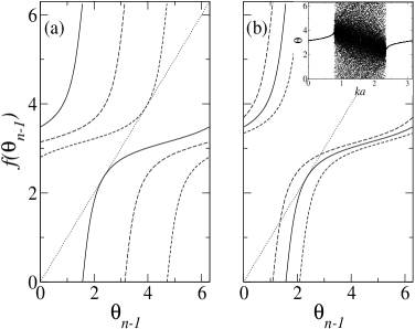
Figure 2: $f(\theta_{n})$ of Eq. (6) for $\epsilon=\frac{1}{4}$: (a) $ka=\pi/4$ (dashed), $2\pi/4$ (long dashed), $3\pi/4$ (continuous), and (b) $ka=2.6$ (long dashed), $3\pi/4$ (continuous), $2.1$ (dashed). The dotted lines correspond to the identity. Inset: Periodic and chaotic attractors.

Information about transport can be obtained from the sensitivity to initial conditions that characterizes the dynamics of the nonlinear map. For finite $n$ it is given by

$$\Xi_{n}\equiv\left|\frac{d\theta_{n}}{d\theta_{0}}\right|\equiv\exp(\Lambda_{1}(n)\ n),$$ (10)

where $\theta_{0}$ is an initial condition and the exponential law after the 2nd identity defines the finite $n$ Lyapunov exponent $\Lambda_{1}(n)$. For $n$ large $\Lambda_{1}(n)$ becomes the Lyapunov exponent $\lambda_{1}$, a number independent of $\theta_{0}$ that according to its sign characterizes periodic and chaotic attractors. At the tangent bifurcation $\lambda_{1}=0$ and the sensitivity adopts instead a $q$-exponential form (see below) Baldovin2002 ; qexponential . From Eqs. (5), (10) and Eq. (6) (and $t_{n}=\frac{1}{2}(e^{i\theta_{n}}-e^{i\theta_{n}^{\prime}})$) we obtain the recursion formula

$$g_{n} = g_{n-1}\exp(\Lambda_{1}(n)\ n)\exp(\Lambda_{1}^{\prime}(n)\ n),$$ (11)

$$\Lambda_{1}(n) = \ln\frac{\epsilon}{1-\epsilon-\sqrt{1-2\epsilon}\cos(\theta_{n}+2ka)},$$ (12)

where $\Lambda_{1}^{\prime}(n)$ is given by Eq. (12) with $\theta_{n}$ replaced by $\theta_{n}^{\prime}$. We note that $\Lambda_{1}$ and $\Lambda_{1}^{\prime}$, and hence $g_{n}$, do not depend on the initial conditions $\theta_{0}$ and $\theta_{0}^{\prime}$. The Lyapunov exponent $\lambda_{1}$ is given by Eq. (12) with $\theta_{n}$ replaced by $\theta_{\infty}$.

The dynamical properties of the map (6) translate into the following network properties: i) In relation to the attractors of period one that take place along $0\leq ka<k_{c}a$ and $k_{c^{\prime}}a<ka\leq\pi$, we corroborate from Eqs. (8) and (12) that $\lambda_{1}$ is negative and therefore the conductance $g_{n}$ decays exponentially with system size $n$, $g_{n}=\exp(2\lambda_{1}n)$, implying localization, the localization length being $\zeta_{1}=a/|\lambda_{1}|$. In the left panel of Fig. 3 we see a clear exponential decay of $g_{n}$ as a function of $n$ at $ka=0.5$, where we compare $g_{n}$ computed directly from Eq. (5) with that obtained from $\lambda_{1}$. We notice that the conductance for the localized states of an ordered system displays the same behavior as that in the insulating regime of a disordered wire in quasi-one-dimensional configuration Beenakker1997 . ii) With respect to the chaotic attractors that occur in the interval $k_{c}a<ka<k_{c^{\prime}}a$ we observe that $\lambda_{1}$ becomes positive and the recursion relation Eq. (11) does not let $g_{n}$ decay but makes it oscillate with $n$ (not shown here) indicating that conduction takes place. In our model $g_{n}$ does not scale with system size as in the metallic regime of quasi-one-dimensional disordered wire where Ohm’s law is satisfied Beenakker1997 . In the parameter region where the map is incipiently chaotic, say $ka\gtrsim k_{c}a$, the network grows with $n$ with an insulator character, but interrupted for other intermediate values of $n$ by conducting crystals. In the map dynamics these are the laminar episodes separated by chaotic bursts in intermittent trajectories.

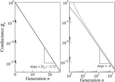
Figure 3: Conductance as a function of generation for $\epsilon=\frac{1}{4}$: $ka=0.5$ (left panel) and $ka=\pi/4$ (right panel). Continuous lines represent $g_{n}$ obtained directly from the map through Eq. (5) while dotted lines correspond to $g_{n}=\exp(2\lambda_{1}n)$ and $g_{n}=\exp_{3/2}(2\lambda_{3/2}n)$ for left panel and right panel, respectively. The two curves in (b) differ because of a proportionality factor, See Eq. (14).

The most distinct outcome of our treatment is the description obtained of the mobility edge from the dynamics at the critical attractors located at $ka=k_{c^{\prime}}a$ and $ka=k_{c}a$. There $\lambda_{1}=0$ and according to Eq. (11) not much can be said about the size dependence of the conductance when $n\gg 1$. However we can use to our advantage the known properties of the anomalous dynamics occurring at these attractors once they are identified as tangent bifurcations [see Fig. 2(b) for $ka=3\pi/4$]. At a tangent bifurcation of general nonlinearity $z>1$ the sensitivity obeys a $q$-exponential law for large $n$ Baldovin2002 ,

$$\xi_{n}=\Xi_{n\gg 1}=\exp_{q}(\lambda_{q}n)\equiv[1-(q-1)\lambda_{q}n]^{\mp\frac{1}{q-1}},$$ (13)

where $\lambda_{q}$ is a $q$-generalized Lyapunov coefficient given by $\lambda_{q}=\mp zu$, $q=2-1/z$, where $u$ is the leading term of the expansion up to order $z$ of $\theta_{n}$ close to $\theta_{c}$ (or $\theta_{c^{\prime}}$); i.e. $\theta_{n}-\theta_{c}=(\theta_{n-1}-\theta_{c})+u\,|\theta_{n-1}-\theta_{c}|^{z}+\cdots$. The minus and plus signs in Eq. (13) and in $\lambda_{q}$ correspond to trajectories at the left and right, respectively, of the point of tangency $\theta_{c}$. Eq. (13) implies power-law decay of $\xi_{n}$ with $n$ when $\theta_{n}-\theta_{c}<0$ and faster than exponential growth when $\theta_{n}-\theta_{c}>0$. (We recall that any choice of $S_{0}$ other that the Pauli matrix translates into another initial condition for the map). By making the expansion around $\theta_{c}$ (or $\theta_{c^{\prime}}$) for our map (6) we find (as evidently anticipated) $z=2$ implying $q=3/2$, $u=\sqrt{(1-2\epsilon)/2\epsilon}$, and the $q$-generalized Lyapunov exponent is $\lambda_{3/2}=-2\sqrt{(1-2\epsilon)/2\epsilon}$. Following the same steps that lead to Eq. (11), the recursion relation for $g_{n}$ at each bifurcation point takes the form $g_{n}=g_{n-1}\exp_{3/2}(\Lambda_{3/2}(n)n)\exp_{3/2}(\Lambda_{3/2}^{\prime}(n)n)$, so that when $\theta_{n}-\theta_{c}<0$ (see Eq. (13)), $g_{n}=\exp_{3/2}(2\lambda_{3/2}n)$, or

$$g_{n}\propto\left(1-\frac{1}{2}\lambda_{3/2}n\right)^{-4}.$$ (14)

In the right panel of Fig. 3 we compare the results from Eq. (5) (continuous line) and Eq. (14) (dashed line). It is clear that $g_{n}$ decays as a power law (with quartic exponent) rather than the exponential in the insulating phase. We enphasize that a localization length given by $\zeta_{3/2}=a/\lambda_{3/2}$ can still be defined at the mobility edge. To our knowledge this property has not been reported before. When $\theta_{n}-\theta_{c}>0$, $\lambda_{3/2}=2\sqrt{(1-2\epsilon)/2\epsilon}>0$ and the recursion relation for $g_{n}$ describes, as the result of the diverging duration of the laminar episodes of intermittency, large $n$ intervals of vanishing $g_{n}$ between increasingly large spike oscillations.

In summary, we can draw significant conclusions about electronic transport from our study. These arise naturally when considering the dynamical properties of the equivalent nonlinear map near or at the intermittency transition to chaos. Since iteration time in the map translates into the generation $n$ of the network, time evolution means growth of system size, reaching the thermodynamic limit (and true self similarity) when $n\rightarrow\infty$. In that limit, windows of period one separated by a chaotic band correspond, respectively, to localized and extended electronic states. Further, in the referred parameter ($ka$, $\epsilon$) regions the conductance $g_{n}$ of the model crystal shows either an exponential decay with system size, with localization length given by $\zeta_{1}$ (as in the case of a quasi-one-dimensional disordered wire Beenakker1997 ), or an oscillating property signalling conducting states. The pair of tangent bifurcation points of the map correspond to the band or mobility edges that separate conductor from insulator behavior. At these bifurcations the sensitivity to initial conditions $\xi_{n}$ exhibits either power-law decay (when $\theta_{0}<\theta_{c^{\prime}}$ or $\theta_{0}>\theta_{c}$) or faster than exponential increase ($\theta_{c^{\prime}}<\theta_{0}<\theta_{c}$) and consequently the conductance inherits comparable decay or variability with system size $n$. Notably, as we have seen we can still define a localization length, the $q$-generalized localization length $\zeta_{q}$ with a fixed value of $q=3/2$. This expression is universal, i.e. it is satisfied by all maps that in the neighborhood of the point of tangency have quadratic term, i.e. $z=2$ Baldovin2002 . This quantity can be obtained directly by evaluation of $g_{n}$ (in Eq. (5)) when $n\rightarrow\infty$. At the mobility edge $\zeta_{1}^{-1}=-\lim_{n\rightarrow\infty}n^{-1}\ln g_{n}$ vanishes because $\ln g_{n}$ no longer decreases linearly with $n$, as it is the case in the insulating phase. However, use of $\zeta_{q}^{-1}=-\lim_{n\rightarrow\infty}n^{-1}\ln_{q}g_{n}$ leads to a finite number for one particular value of $q$, $q=3/2$, when the degree of deformation $q$ in the $q$-logarithm restores linear behavior. Otherwise $\zeta_{q}$ vanishes or diverges.

In spite of the unusual features of the double Cayley tree transport model, the complete set of exact solutions derived from it provides a comprehensive picture about non-exponential behavior of central quantities like the conductance at the transition between the insulator and conductor regimes.

We are indebted to P. A. Mello for pointing out and introducing us to the model and techniques to study the mobility edge presented here. AR recognizes support by DGAPA-UNAM and CONACYT (Mexican agencies).

References

- (1) We chose to call here mobility edge, usually employed in reference to disordered systems, the transition between localized and extended electronic states in regular self-similar networks.
- (2) F. Baldovin, A. Robledo, Europhys. Lett. 60, 518 (2002).
- (3) E. Mayoral, A. Robledo, Phys. Rev. E 72, 026209 (2005).
- (4) A. Robledo, L. G. Moyano, Phys. Rev. E 77, 036213 (2008).
- (5) P. G. Harper, Proc. Phys. Soc. London, Sect. A 68, 874 (1955).
- (6) J. A. Ketoja, I. I. Satija, Physica D 109, 70 (1997).
- (7) J. P. Straley, J. Phys. C 10, 3009 (1977).
- (8) R. Abou-Chacra, P. W. Anderson, D. J. Thouless, J. Phys. C 6, 1734 (1973).
- (9) B. Shapiro, Phys. Rev. Lett. 50, 747 (1983).
- (10) N. Zekri, A. Brezini, Phys. Stat. Solidi B 133, 463 (1986).
- (11) Y. Avishai, J. M. Luck, Phys. Rev. B 45, 1074 (1992).
- (12) M. Horvat, T. Prosen, J. Phys. A: Math Theor. 40, 11593 (2007).
- (13) M. Sade, T. Kalisky, S. Havlin, R. Berkovits, Phys. Rev. E 72, 066123 (2005).
- (14) M. Martínez, P. A. Mello, Phys. Rev. E 63, 016205 (2000).
- (15) M. Büttiker, Y. Imry, M. Ya. Azbel, Phys. Rev. A 30, 1982 (1984).
- (16) R. Landauer, J. Phys.: Condens. Matter 1, 8099 (1989).
- (17) M. Büttiker, IBM J. Res. Dev. 32, 317 (1988).
- (18) The -exponential and its inverse the -logarithm are defined, respectively, as for , and for . The ordinary exponential and logarithm are recovered when .
- (19) C. W. J. Beenakker, Rev. Mod. Phys. 69, 731 (1997).