Soft interactions in Herwig++

Abstract

We describe the recent developments to extend the multi-parton interaction model of underlying events in Herwig++ into the soft, non-perturbative, regime. This allows the program to describe also minimum bias collisions in which there is no hard interaction, for the first time. It is publicly available from versions 2.3 onwards and describes the Tevatron underlying event and minimum bias data. The extrapolations to the LHC nevertheless suffer considerable ambiguity, as we discuss.

1 Introduction

In this talk, we will summarize the development of a new model for the underlying event in Herwig++, extending the previous perturbative multi-parton interaction (MPI) model down into the soft non-perturbative region. This allows minimum bias collisions to be simulated by Herwig++ for the first time.

We begin, though, by mentioning a few of the features that accompanied it in the release of Herwig++[1] version 2.3[2] in December 2008, which include NLO corrections in the POWHEG scheme for single W and Z production[3], and Higgs production[4]. Lepton–hadron scattering processes have been included for the first time. The simulation of physics beyond the standard model (BSM) has been extended to include a much wider range of 3-body decays and off-shell effects[5]. The treatment of baryon decays has been extended to match the sophistication of meson and tau decays, including off-shell and form factor effects and spin correlations. Finally, in addition to the soft interactions discussed here, the MPI model has been extended to include the possibility of selecting additional scatters of arbitrary type, which can be important backgrounds to BSM signatures for which the single-scattering backgrounds are small, for example two like-sign Drell-Yan W productions[6].

The semi-hard MPI model was implemented in Herwig++ version 2.1[7]. It allows for the simulation of underlying events with perturbative scatters with $p_{t}>p_{t}^{\rm min}$ according to the standard QCD matrix elements with standard PDFs, dressed by parton showers that, in the initial state, account for the modifications of the proton structure due to momentum and flavour conservation. It essentially re-implemented the existing Jimmy algorithm[8] that worked with the fortran HERWIG generator[9], but gave a significantly better description of the CDF data on the underlying event[10], in part due to a more detailed global tuning[12]. However it was only able to describe the jet production part of the data, above about 20 GeV, and not the minimum bias part, owing to a lack of soft scatters below $p_{t}^{\rm min}$. A possible extension into the soft regime was first discussed in Ref. [13], but we have provided the first robust implementation of it, described in detail in Ref. [6]. It is somewhat complementary to the approach used in Pythia[14, 15], where the perturbative scatters are extended into the soft region through the use of a smooth non-perturbative modification. However, we make a stronger connection with information on total and elastic scattering cross sections, available through the eikonal formalism, to place constraints on our non-perturbative parameters[16].

Figure 1: Total cross sections (black) in the two parameterizations of Donnachie and Landshoff[17, 18]. In blue the QCD jet production cross section above 2 GeV is shown.

In the remainder of this introduction, we recap the basics of the eikonal model and recall the results of the perturbative MPI model that we had previously implemented in Herwig++, before showing how to extend it into the soft region. In Sect. 2 we discuss the constraints that can be placed on the model by the connection with hadronic scattering, and in Sect. 3 we show the predictions for final state properties.

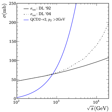
The starting point for the MPI model is the observation that the inclusive cross section for perturbative parton scattering may exceed the total hadron–hadron cross section. We show an example in Fig. 1, with two of the total cross section parameterizations we will be using. The origin of the steep rise in the partonic cross section is the proliferation of partons expected at small $x$. The excess of the partonic scattering cross section over the total cross section simply implies that there is on average more than one parton scattering per inelastic hadronic collision, $\bar{n}=\sigma_{\rm jet}/\sigma_{\rm inel}$. Since the majority of scatters come from very small $x$ partons, they consume relatively little energy and it is a good approximation to treat them as quasi-independent.

From the optical theorem, one derives a relationship between the Fourier transform of the elastic amplitude $a({\bf b},s)$ and the inelastic cross section via the eikonal function, $\chi({\bf b},s)$,

$$a({\bf b},s)\equiv\frac{1}{2i}\left[\>e^{-\chi({\bf b},s)}\>-1\right]\qquad\longrightarrow\qquad\sigma_{\rm inel}=\int{\rm d}^{2}{\bf b}\left[1-\>e^{-2\chi({\bf b},s)}\>\right].$$ (1)

One can construct a QCD prediction for the eikonal function by assuming that multiple scatters are independent, and that the partons that participate in them are distributed across the face of the hadron with some impact parameter distribution $G({\bf b})$ that is independent of their longitudinal momentum,

$$\chi_{\rm QCD}({\bf b},s)={\textstyle\frac{1}{2}}\,A({\bf b})\,\sigma^{\rm inc}_{\rm hard}(s),\qquad\qquad A({\bf b})=\int{\rm d}^{2}{\bf b}^{\prime}\,G({\bf b}^{\prime})\,G({\bf b}-{\bf b}^{\prime}),$$ (2)

where $\sigma^{\rm inc}_{\rm hard}$ is the inclusive partonic scattering cross section, which is given by the conventional perturbative calculation.

In the original Jimmy model and its Herwig++ reimplementation, these formulae are implemented in a straightforward way, with the hard cross section defined by a strict cut, $p_{t}>p_{t}^{\rm min}$ and the matter distribution given by the Fourier transform of the electromagnetic form factor,

$$G({\bf b})=\int\frac{{\rm d}^{2}{\bf k}}{(2\pi)^{2}}\;\frac{\>e^{i\,{\bf k}\cdot{\bf b}}\>}{(1+{\bf k}^{2}/\mu^{2})^{2}},$$ (3)

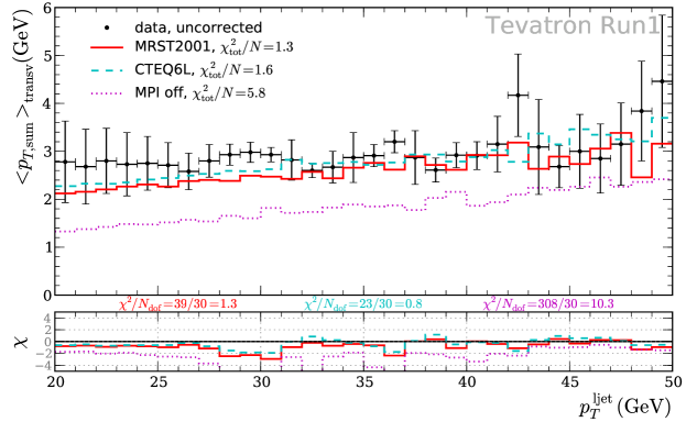
with, to reflect the fact that the distribution of soft partons might not be the same as that of electromagnetic charge, $\mu^{2}$ considered to be a free parameter and not fixed to its electromagnetic value $0.71\text{ GeV}^{2}$. Compared to a Gaussian of the same width, this distribution has both a stronger peak and a broader tail so it is somewhat similar to the double-Gaussian form used in Pythia[19]. In Ref. [16], we explicitly showed that the two result in similar distributions, if their widths are fixed to be equal, except very far out in the tails. $\mu^{2}$ and $p_{t}^{\rm min}$ are the main adjustable parameters of the model and, allowing them to vary freely, one can get a good description of the CDF underlying event data, as shown in Fig. 2. The choice of parton distribution function can also be seen to have a small but significant effect.

Figure 2: Multiplicity and $p_{t}^{\rm sum}$ in the transverse region. CDF data are shown as black circles, Herwig++ without MPI as magenta dots, with MPI using MRST [20] PDFs as solid red and with CTEQ6L [21] as cyan dashed. The lower plot shows the statistical significance of the disagreement between the Monte Carlo predictions and the data. The legend on the upper plot shows the total $\chi^{2}$ for all observables, whereas the lower plot for each observable has its $\chi^{2}$ values.

The main shortcoming of this model is that it does not contain soft scatters and hence cannot describe very low $p_{t}$ jet production or minimum bias collisions. In Ref. [13] it was proposed to remedy this, by extending the concept of independent partonic scatters right down into the infrared region. One can therefore write the eikonal function as the incoherent sum of the QCD component we already computed and a soft component,

$$\chi_{\rm tot}({\bf b},s)=\chi_{\rm QCD}({\bf b},s)+\chi_{\rm soft}({\bf b},s)={\textstyle\frac{1}{2}}\Bigl{(}A({\bf b})\,\sigma^{\rm inc}_{\rm hard}(s)+A_{\rm soft}({\bf b})\,\sigma^{\rm inc}_{\rm soft}(s)\Bigr{)},$$ (4)

where $\sigma^{\rm inc}_{\rm soft}$ is an unknown partonic soft scattering cross section. As a first simplest model, we assume that the matter distributions are the same, $A_{\rm soft}({\bf b})=A({\bf b})$, although we relax this condition later. By taking the eikonal approach seriously, we can trade the unknown soft cross section for the unknown total hadronic cross section,

$$\sigma_{\rm tot}(s)=2\int{\rm d}^{2}{\bf b}\left[1-\>e^{-\frac{1}{2}A({\bf b})(\sigma^{\rm inc}_{\rm hard}(s)+\sigma^{\rm inc}_{\rm soft}(s))}\>\right].$$ (5)

Knowing the total cross section, for a given matter distribution and hard cross section (implied by $p_{t}^{\rm min}$ and the PDF choice) the soft cross section is then determined. In order to make predictions for energies higher than the Tevatron, we consider three predictions of the total cross section: 1) the standard Donnachie–Landshoff parameterization[17]; 2) the latter for the energy dependence but with the normalization fixed by the CDF measurement[22]; and 3) the newer Donnachie–Landshoff model with a hard component[18]. Of course once we have an experimental measurement from the LHC we would use that for our predictions. In this way, our simple hard+soft model has no more free parameters than our hard model and we can tune $\mu^{2}$ and $p_{t}^{\rm min}$. Before doing this, we present the results of Ref. [16], in which we considered the theoretical constraints that could be put on these parameters.

2 Analytical constraints

2.1 Simple model

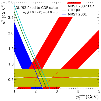
Within our model we want $\sigma^{\rm inc}_{\rm soft}$ to correspond to a physical cross section. It must therefore be positive. This therefore places constraints on the $\mu^{2}$–$p_{t}^{\rm min}$ plane: a lower bound on $p_{t}^{\rm min}$ for a given value of $\mu^{2}$. These are shown for the Tevatron on the left-hand side of Fig. 3 as the solid lines for three different PDF sets: the two shown previously and MRST LO*[23]. Since in the eikonal model the total and inelastic cross sections are related to the elastic one, we can also place constraints from the elastic slope parameter, which has been measured by CDF[22, 24]:

$$b_{\rm el}(s)\equiv\left[\frac{\rm d}{{\rm d}t}\left(\ln\frac{\rm d\sigma_{\rm el}}{{\rm d}t}\right)\right]_{t=0}=\frac{1}{\sigma_{\rm tot}}\int{\rm d}^{2}{\bf b}\,b^{2}\left[1-\>e^{-\chi_{\rm tot}({\bf b},s)}\>\right]=(17\pm 0.25)\text{ GeV}^{-2}.$$ (6)

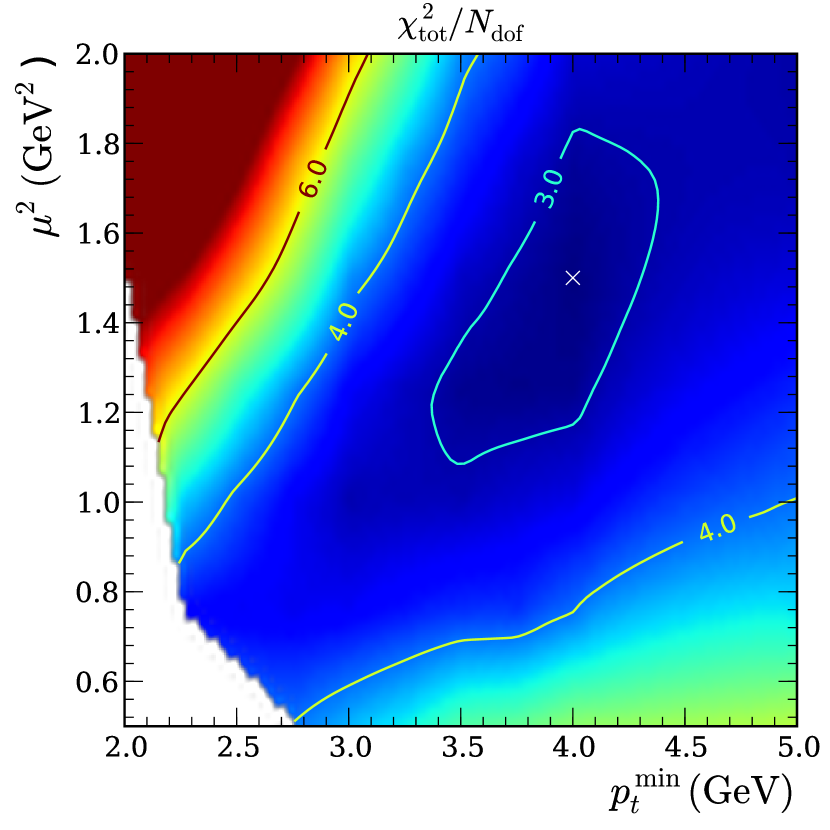
This rather precise measurement directly constrains $\mu^{2}$ in our simple model and rules out all but a very narrow strip of the parameter space. Finally, we consider the parameter space of the fit to final-state data. Although there is a preferred point in the parameter space, the tuning of both the hard-only model[12] and the hard+soft model shown below indicates a strong correlation between the two parameters and there is a broad region of acceptable parameter values, which we show in Fig. 3 by the region edged by red bands. Between the different constraints we have only a very small allowed region of parameter space.

Figure 3: Left: The parameter space of the simple eikonal model at the Tevatron. The solid curves come from $\sigma^{\rm inc}_{\rm soft}>0$ for three different PDF sets. The horizontal lines come from $b_{\rm el}=16.98\pm 0.25\text{ GeV}^{-2}$[22, 24]. The excluded regions are shaded. The dashed lines indicate the preferred parameter ranges from the fit to Tevatron final-state data[12]. Right: The equivalent plot for the LHC. The additional (dashed) constraints come from requiring the total number of scatters to be less than 10.

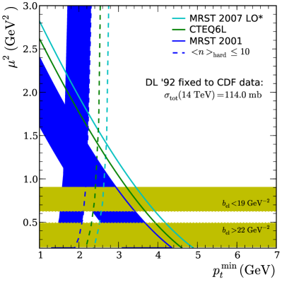
At the LHC the picture is similar, although the constraint $\sigma^{\rm inc}_{\rm soft}>0$ is considerably more restrictive (note the difference in range of the $x$ axes of the two plots). Different models predict $b_{\rm el}$ in the range 19 to 22$\text{ GeV}^{-2}$ translating into a slightly wider horizontal band. Finally, although we do not have final-state data to compare to, in order to simulate self-consistent final states at all we find that we must prevent the multiplicity of scatters becoming too high. While precisely where we place this cut is arbitrary, we indicate it by shading the region in which the mean number of scatters is greater than 10. This plot is shown for the central of the three total LHC cross section predictions we consider – it is qualitatively similar for the other two, although the different constraints move somewhat.

Comparing the two plots in Fig. 3, we come to the realization that, from these theoretical constraints together with the fit to the Tevatron data, we can already rule out the possibility that the parameters of this simple model are energy-independent – there is no region of the plot that is allowed at both energies.

While it could be that the parameters of the MPI model are in fact energy dependent, as advocated by the PYTHIA authors[25], we prefer to let the LHC data decide, by proposing a model that is flexible enough to allow energy-independent or -dependent parameters. The simplest generalization of the above model that achieves this is actually well physically motivated, and we call it the hot-spot model.

2.2 Hot-Spot model

The simple model has other shortcomings, beyond our aesthetic preference to allow the possibility of energy-independent parameters. The values of $\sigma^{\rm inc}_{\rm soft}$ extracted from the predictions of $\sigma_{\rm tot}$[16], have rather strange energy dependence, being quite sensitive to precise details of the matter distribution, parameter choice, cross section prediction and PDF set and, in most cases, having a steeply rising dependence on energy, much steeper than one would like to imagine for a purely soft cross section. Moreover, the value of $\mu^{2}$ extracted from $b_{\rm el}$ is in contradiction with that extracted from CDF’s measurement[26] of double-parton scattering, which yields $\mu^{2}=3.0\pm 0.5\text{ GeV}^{2}$.

All of these shortcomings can be circumvented by allowing the matter distribution to be different for soft and hard scatters. As a next simplest model, we keep the same form for each, but allow the $\mu^{2}$ values to be different. We again fix the additional free parameter, this time to a fixed value of $b_{\rm el}$. That is, once $\sigma_{\rm tot}$ and $b_{\rm el}$ are measured at some energy, the non-perturbative parameters of our model, $\sigma^{\rm inc}_{\rm soft}$ and $\mu^{2}_{\rm soft}$ are known. Since it will turn out that our preferred value of $\mu^{2}$ is significantly larger than the extracted value of $\mu^{2}_{\rm soft}$, we call this a hot-spot model: soft partons have a relatively broad distribution, actually similar to the electromagnetic form factor, while semi-hard partons (typically still small $x$, but probed at momentum scales above $p_{t}^{\rm min}$) are concentrated into smaller denser regions within the proton.

Having used one constraint to fix an additional parameter, there is only one constraint in the parameter space, shown in Fig. 4 for the Tevatron and LHC.

Figure 4: Parameter space of the improved eikonal model for the Tevatron (left) and LHC (right). The solid curves impose a minimum allowed value of $\mu^{2}$, for a given value of $p_{t}^{\rm min}$ by requiring a valid description of $\sigma_{\rm tot}$ and $b_{\rm el}$ with positive $\sigma^{\rm inc}_{\rm soft}$. The excluded regions are shaded. We used the MRST 2001 LO[20] PDFs for these plots.

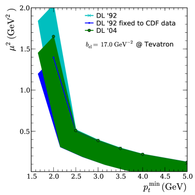
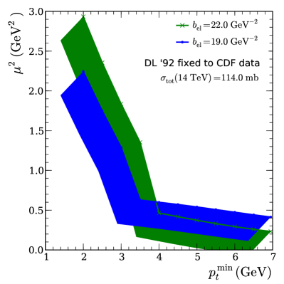
The model has much more freedom than the simple one, with much of the parameter space allowed, and with ample overlap between the allowed regions at the two energies.

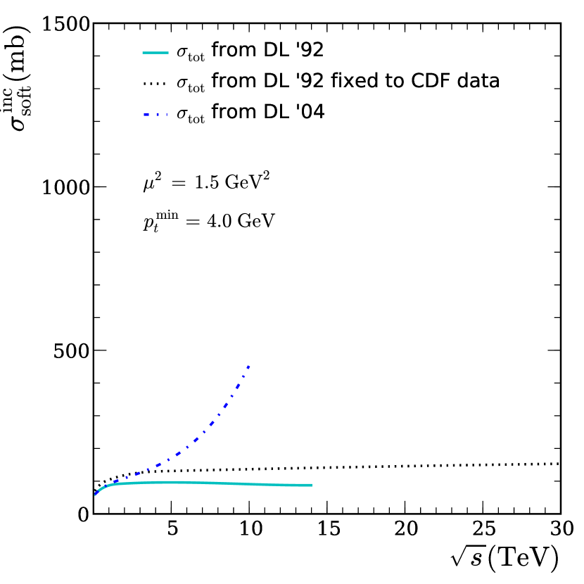
Another nice feature of this model is the energy-dependence of $\sigma^{\rm inc}_{\rm soft}$ it implies, shown in Fig. 6. At least for the standard Donnachie–Landshoff energy dependence, it corresponds to a very slow increase, almost constant, in-keeping with one’s expectations of a soft cross section.

3 Final states

We have implemented this model into Herwig++. There are many additional details that we do not go into here[6], but wherever possible, the treatment of soft scatters is kept as similar as possible to that of semi-hard scatters, to make for a smooth matching. In particular, for the transverse momentum dependence, we make the distribution of $p_{t}^{2}$ a Gaussian centred on zero, whose integral over the range zero to $p_{t}^{\rm min}$ is given by $\sigma^{\rm inc}_{\rm soft}$ and whose width is adjusted such that ${\rm d}\sigma/{\rm d}p_{t}$ is continuous at $p_{t}^{\rm min}$. $p_{t}^{\rm min}$ is therefore seen to be not a cutoff, as it is in the Jimmy model, but a matching scale, where the model makes a relatively smooth transition between perturbative and non-perturbative treatments of the same phenomena, in a similar spirit to the model of Ref. [29] for transverse momentum in initial-state radiation.

The model actually exhibits a curious feature in its $p_{t}$ dependence, first observed in Ref. [13]. With the typical parameter values that are preferred by the data, ${\rm d}\sigma/{\rm d}p_{t}$ is large enough, and $\sigma^{\rm inc}_{\rm soft}$ small enough, that the soft distribution is not actually a Gaussian but an inverted Gaussian: its width-squared parameter is negative. The result is that the transverse momentum of scatters is dominated by the region around $p_{t}^{\rm min}$ and not by the truly non-perturbative region $p_{t}\to 0$. This adds to the self-consistency of the model, justifying the use of an independent partonic scattering picture even for soft non-perturbative collisions.

With the model in hand, we can repeat the tune to the CDF data on the underlying event. Unlike with the semi-hard model, we now fit the data right down to zero leading jet momentum. The result is shown in Fig. 6, which is qualitatively similar to the one for the semi-hard model.

Figure 5: $\sigma^{\rm inc}_{\rm soft}$ as a function of energy. Each of the three different curves shows the soft cross section that would appear when the respective parameterization for the total cross section is used. Curves that do not reach out to 30 TeV correspond to parameter choices that are unable to reproduce $\sigma_{\rm tot}$ and $b_{\rm el}$ correctly at these energies.

Figure 6: Contour plots for the $\chi^{2}$ per degree of freedom for the fit to the CDF underlying event data. The cross indicates the location of our preferred tune and the white area consists of parameter choices where the elastic $t$-slope and the total cross section cannot be reproduced simultaneously.

The description of the data in the transverse region is shown in Fig. 7.

Figure 7: Multiplicity and $p_{t}^{\rm sum}$ in the transverse region. CDF data are shown as black circles. The histograms show Herwig++ with the improved model for semi-hard and soft additional scatters using the MRST 2001 LO [20] PDFs for three different parameter sets. The lower plot shows the ratio Monte Carlo to data and the data error band. The legend shows the total $\chi^{2}$ for all observables.

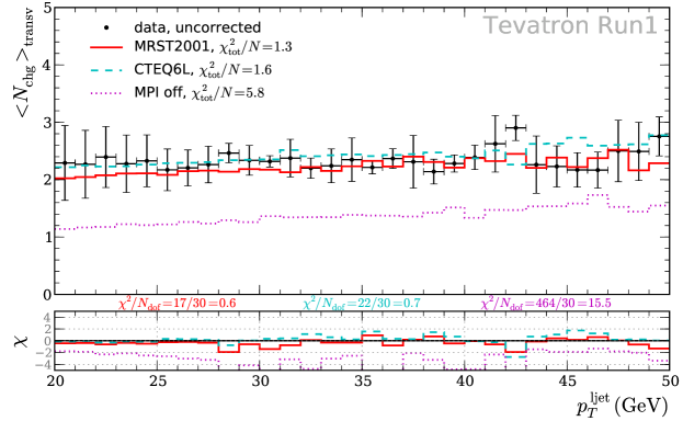
It can be seen to be reasonable in the lower transverse momentum region, although certainly still not as good as at higher transverse momenta.

The discrepancy in the lowest few bins may be related to another deficiency of our model. According to the eikonal model, the inelastic cross section should include all final states that are not exactly elastic, while our simulation of them generates only non-diffractive events in which colour is exchanged between the two protons and hence a significant number of final-state hadrons are produced. While single-diffractive-dissociation events would not be triggered on experimentally, double-diffractive-dissociation events, in which both protons break up but do not exchange colour across the central region of the event, would, and would lead to extremely quiet events with low leading jet $p_{t}$ and low central multiplicity, which are not present in our sample. In Ref. [6] we have checked that these bins are not pulling our tune significantly by repeating it without them. The overall chi-squared is significantly smaller, but the best fit point and chi-squared contours are similar.

4 Conclusions

We have reviewed the basis of the semi-hard MPI model that we previously implemented in Herwig++, and motivated its extension to a soft component. Through the connection with the total and elastic cross sections provided by the eikonal model and optical theorem, we have placed significant constraints on the simplest soft model. We have shown that these constraints can be relaxed by invoking a hot-spot model in which the spatial distributions of soft and semi-hard partons are different. Finally, we have implemented this model and shown that it gives a reasonable description of the minimum bias data, for the first time in Herwig++. Nevertheless, there is still room for improvement, particularly in the very low $p_{t}$ region and several avenues for further study present themselves, not least the diffractive component already mentioned, and the role of colour correlations, which were argued to be very important in Ref. [15], but which seem to be less so in the current Herwig++ implementation[6].

Despite the successful description of Tevatron data, the extrapolation to the LHC suffers from considerable uncertainty. The unknown value of the total cross section, which determines the non-perturbative parameters in our model, plays a crucial role, but even once this and the elastic slope parameter have been directly measured, the region of allowed parameter space is still large. Although we prefer a model in which the parameters are energy independent, ultimately only data will tell us whether this is the case. Finally, even once the underlying event data have been measured, the parameters will not be fully tied down, due to their entanglement with the PDFs. We eagerly await the LHC data to guide us.

References

- [1] M. Bähr et al., Eur. Phys. J. C58, 639 (2008). 0803.0883
- [2] M. Bähr et al., Herwig++ 2.3 Release Note, 2008. 0812.0529
- [3] K. Hamilton, P. Richardson, and J. Tully, JHEP 10, 015 (2008). 0806.0290
- [4] K. Hamilton, P. Richardson, and J. Tully, JHEP 04, 116 (2009). 0903.4345
- [5] M. A. Gigg and P. Richardson, Simulation of Finite Width Effects in Physics Beyond the Standard Model, 2008. 0805.3037
- [6] Bähr, M., Underlying Event Simulation in the Herwig++ Event Generator. Ph.D. Thesis, Institut für Theoretische Physik, Universität Karlsruhe, Dec. 2008
- [7] M. Bähr et al., Herwig++ 2.1 release note, 2007. 0711.3137
- [8] J. M. Butterworth, J. R. Forshaw, and M. H. Seymour, Z. Phys. C72, 637 (1996). hep-ph/9601371
- [9] G. Corcella et al., JHEP 01, 010 (2001). hep-ph/0011363
- [10] CDF Collaboration, A. A. Affolder et al., Phys. Rev. D65, 092002 (2002)
- [11] CDF Collaboration, D. E. Acosta et al., Phys. Rev. D70, 072002 (2004). hep-ex/0404004
- [12] M. Bähr, S. Gieseke, and M. H. Seymour, JHEP 07, 076 (2008). 0803.3633
- [13] I. Borozan and M. H. Seymour, JHEP 09, 015 (2002). hep-ph/0207283
- [14] T. Sjöstrand and M. van Zijl, Phys. Rev. D36, 2019 (1987)
- [15] T. Sjöstrand and P. Z. Skands, JHEP 03, 053 (2004). hep-ph/0402078
- [16] M. Bähr, J. M. Butterworth, and M. H. Seymour, JHEP 01, 065 (2009). 0806.2949
- [17] A. Donnachie and P. V. Landshoff, Phys. Lett. B296, 227 (1992). hep-ph/9209205
- [18] A. Donnachie and P. V. Landshoff, Phys. Lett. B595, 393 (2004). hep-ph/0402081
- [19] T. Sjöstrand, S. Mrenna, and P. Skands, JHEP 05, 026 (2006). hep-ph/0603175
- [20] A. D. Martin, R. G. Roberts, W. J. Stirling, and R. S. Thorne, Eur. Phys. J. C23, 73 (2002). hep-ph/0110215
- [21] J. Pumplin et al., JHEP 07, 012 (2002). hep-ph/0201195
- [22] CDF Collaboration, F. Abe et al., Phys. Rev. D50, 5550 (1994)
- [23] A. Sherstnev and R. S. Thorne, Eur. Phys. J. C55, 553 (2008). 0711.2473
- [24] CDF Collaboration, F. Abe et al., Phys. Rev. D50, 5518 (1994)
- [25] J. Dischler and T. Sjöstrand, Eur. Phys. J. direct C3, 2 (2001). hep-ph/0011282
- [26] CDF Collaboration, F. Abe et al., Phys. Rev. D56, 3811 (1997)
- [27] D. Treleani, Phys. Rev. D76, 076006 (2007). 0708.2603
- [28] M. Bähr and M. H. Seymour, Comment on CDF’s extraction of from their measurement of double parton scattering, 2009. In preparation
- [29] S. Gieseke, M. H. Seymour, and A. Siódmok, JHEP 06, 001 (2008). 0712.1199.