Eulerian and Lagrangian pictures of non-equilibrium diffusions

Abstract

We show that a non-equilibrium diffusive dynamics in a finite-dimensional space takes in the Lagrangian frame of its mean local velocity an equilibrium form with the detailed balance property. This explains the equilibrium nature of the fluctuation-dissipation relations in that frame observed previously. The general considerations are illustrated on few examples of stochastic particle dynamics.

1 Introduction

In the last decades, non-equilibrium statistical mechanics has been a subject of intensive studies. One of the multiple aims of the research is the understanding of essential differences between the equilibrium and non-equilibrium dynamics. This is the question that we shall address below. In the modelling of statistical-mechanical dynamics, an important role has been played by stochastic Markov processes. Although largely idealized, they often provide a sufficiently realistic description of experimental situations and have traditionally served as a playground for both theoretical considerations and numerical studies. The Markov processes corresponding to the equilibrium dynamics are characterized by the detailed balance property assuring that the net probability fluxes between micro-states of the system vanish. On the other hand, in the non-equilibrium Markov dynamics, the detailed balance is broken and there are non-zero probability fluxes even in a stationary situation.

In the present paper, we shall consider only diffusive processes, discarding Markov processes with discrete time or random jumps. For such systems, the detailed balance can be expressed as the vanishing of the probability current that is non-zero in the non-equilibrium situations. It is convenient to represent the probability current in a hydrodynamical form as the instantaneous probability density of the process multiplied by the mean local velocity. The latter is the average instantaneous velocity of the process conditioned to pass through a given point. It will play the main role in what follows.

In the past, there have been many attempts to apply ideas from statistical mechanics to the hydrodynamics of turbulent flows. The success was limited by the fact that most methods of statistical physics had been developed for systems in or close to equilibrium whereas developed turbulence is a far-from-equilibrium phenomenon. Here we shall follow a reversed strategy, applying an idea from hydrodynamics to non-equilibrium statistical mechanics. There is a long tradition (going back to Lagrange) to describe the evolution of hydrodynamical fields in the Lagrangian frame that moves with fluid particles [21]. It is believed that such a description makes the intrinsic features of fluid dynamics at small scales more directly accessible than in the Eulerian (i.e. laboratory) frame. This is particularly true about the hydrodynamical advection that gains a simple representation in the Lagrangian frame.  The main result of the present paper consists of a simple observation that the non-vanishing probability current in a Markov diffusion may be decoupled from the stochastic dynamics by passing to the Lagrangian frame of the mean local velocity.  More exactly, in the latter frame, the stochastic dynamics, although non-stationary, satisfies the detailed balance condition and the instantaneous probability density of the process does not change in time. The equilibrium-like Lagrangian-frame process does not contain information about the non-vanishing probability current of the original Eulerian-frame process but, if that information is provided independently, the Eulerian-frame process may be reconstructed from the Lagrangian-frame one. In short, the passage to the Lagrangian frame of the mean local velocity re-expresses a non-equilibrium diffusion process as an equilibrium-type one plus the decoupled probability current. To our knowledge, this rather straightforward observation about non-equilibrium diffusions has not been discussed in the literature, although a similar idea was recently employed in the quantum many-body dynamics [32].

The paper consists of seven Sections and four Appendices. Sect. 2 sets the stage and notations by briefly stating the basic definitions relevant for the diffusion processes that we consider. We introduce the notions of the probability current and of the mean local velocity and recall the concept of detailed balance. The crucial Sect. 3 is devoted to the Lagrangian picture of diffusions. We define the Lagrangian frame of the mean local velocity and compute the instantaneous probability density of the Lagrangian-frame process. By working out the stochastic differential equation satisfied by this process, we show that it is a non-stationary diffusion with the detailed balance property. Two simple examples illustrate the general considerations: a diffusion of a particle on a circle in the presence of a constant force and a linear stochastic equation describing a Rouse model of a polymer in shear flows. We also discuss the reconstruction of the original Eulerian-frame process from the Lagrangian-frame one. Sect. 4 is devoted to the Langevin equations with both Hamiltonian and non-conservative forces. In this case, it is convenient to modify the definition of the probability current and the mean local velocity to assure that they vanish in the absence of the non-conservative drift. The main properties of the Lagrangian-frame process are unaffected by this modification. We illustrate the general discussion by the example of a harmonic chain. Sect. 5.2 discusses the extensions of the Fluctuation-Dissipation Theorem to the non-equilibrium situation in the light of the results about the Lagrangian-frame process. These results provide a deeper reason for the observation made in [6], see also [28], that the fluctuation-dissipation relations takes the equilibrium form in the Lagrangian frame of the mean local velocity. In Sect. 6, we point out that important non-equilibrium diffusion processes in infinite-dimensional spaces, like the one-dimensional KPZ equation or the processes describing the large-deviations regime of fluctuations around the hydrodynamical limit of the boundary-driven zero-range particle processes do not possess Lagrangian picture. Finally, Sect. 7 presents our conclusions. Appendices collect some more technical arguments.

Acknowledgements.  The authors thank Gregory Falkovich for discussions. R.C. acknowledge the support of the Koshland Center for Basic Research and K.G. of the project ANR-05-BLAN-0029-03.

2 Eulerian picture of diffusions

2.1 Diffusion processes

We shall begin by considering a general diffusion process $\,x_{t}\,$ in a $\,d$-dimensional (phase-)space $\,{\cal X}\,$ with coordinates $\,(x^{i})$,  of the same type as in ref. [5] that was devoted to the study of fluctuation relations for such processes. The examples we shall have in mind include various types of Langevin dynamics used to model equilibrium and non-equilibrium dynamics as well as the Kraichnan model of turbulent advection [10]. Of the rich theory of diffusion processes, see e.g. [26, 24, 31], we shall need only few basic facts that we collect below. The process $\,x_{t}\,$ is assumed to satisfy the stochastic differential equation (SDE)

$$\dot{x}_{t}\ =\ u_{t}(x_{t})\,+\,\zeta_{t}(x_{t})\,,$$ (2.1)

where $\,\dot{x}_{t}\equiv\frac{dx_{t}}{dt}$  and, on the right hand side, $\,u_{t}(x)\,$ is a time-dependent deterministic vector field (the drift), and $\,\zeta_{t}(x)\,$ is a Gaussian random vector field with mean zero and covariance

$$\big{\langle}\,\zeta^{i}_{t}(x)\ \zeta^{j}_{s}(y)\,\big{\rangle}\ =\ 2\,\delta(t-s)\,D_{t}^{ij}(x,y)\,.$$ (2.2)

Note that $\,\zeta_{t}(x)\,$ is a white noise in time so that Eq. (2.2) requires a choice of a stochastic convention. As in [5], we shall interpret it in the Stratonovich sense to assure that $\,u^{i}_{t}(x)\,$ and $\,\zeta^{i}_{t}(x)\,$ transform as vector fields under a change of coordinates.  The single time expectations of functions of the process $\,x_{t}\,$ evolve according to the equation

$$\frac{d}{{dt}}\,\big{\langle}\,f(x_{t})\,\big{\rangle}\,=\,\big{\langle}\,(L_{t}f)(x_{t})\,\big{\rangle}\,,\ \qquad{\rm where}\,\ \qquad L_{t}\,=\,\hat{u}^{i}_{t}\partial_{i}+\partial_{j}d_{t}^{ij}\partial_{i}$$ (2.3)

with

$$d_{t}^{ij}(x)\,=\,D_{t}^{ij}(x,x)\qquad\hat{u}^{i}_{t}(x)\,=\,u^{i}_{t}(x)\,-\,r^{i}_{t}(x)\,,\qquad r^{i}_{t}(x)\,=\,\partial_{y^{j}}D_{t}^{ij}(x,y)|_{y=x}$$ (2.4)

are the instantaneous generators of the process $\,x_{t}$.  Note the presence of the term $\,r_{t}\,$ correcting the drift and due to the dependence the covariance of $\,\zeta_{t}\,$ on the points in $\,{\cal X}$.  The time evolution of the instantaneous (i.e. single-time) probability density function (PDF) of the process

$$\rho_{t}(x)\ =\ \big{\langle}\,\delta(x-x_{t})\,\big{\rangle}$$ (2.5)

is governed by the formal adjoints $\,L_{t}^{\dagger}\,$ of the generators $\,L_{t}\,$:

$$\partial_{t}\rho_{t}\ =\ L_{t}^{\dagger}\rho_{t}\ =\ -\partial_{i}\big{[}\hat{u}^{i}_{t}\rho_{t}\,-\,d^{ij}_{t}\,\partial_{j}\rho_{t}\big{]}\,.$$ (2.6)

The transition PDF’s of the Markov process $\,x_{t}\,$ given by the conditional expectations

$$P(s,x;t,y)\ =\ \rho_{s}(x)^{-1}\,\big{\langle}\,\delta(x-x_{s})\,\delta(y-x_{t})\,\big{\rangle}$$ (2.7)

with $\,s\leq t\,$ satisfy the Chapman-Kolmogorov composition rule $\ \int P(r,x;s,y)\,P(s,y;t,z)\,dy\,=\,P(r,x;t,z)\$ and the Kolmogorov differential equations

$$\partial_{s}P(s,x;t,y)\ =\ -L_{s}(x)\,P(s,x;t,y)\,,\qquad\partial_{t}P(s,x;t,y)\ =\ L^{\dagger}_{t}(y)\,P(s,x;t,y)\,.$$ (2.8)

The latter, together with the condition $\,P(t,x;t,y)=\delta(x-y)$,  determine the transition probabilities under appropriate regularity assumptions [31].

2.2 Probability current and mean local velocity

Some other basic notions concerning Markov diffusions will play a central role below. The evolution equation (2.6) for the instantaneous PDF (2.5) of the process $\,x_{t}\,$ has the form of the continuity equation

$$\partial_{t}\rho_{t}\ +\ \nabla\cdot j_{t}\ =\ 0$$ (2.9)

with the  probability current

$$j^{i}_{t}\ =\ \big{[}\hat{u}^{i}_{t}\,-\,d^{ij}_{t}\,\partial_{j}\big{]}\rho_{t}$$ (2.10)

whose flux through the boundary of any region $\,{\cal V}\,$ gives the rate of change of the probability that $\,x_{t}\,$ belongs to $\,{\cal V}$.  A more transparent interpretation of the current $\,j_{t}(x)\,$ is given by the formula:

$$j^{i}_{t}(x)\ =\ \lim\limits_{\epsilon\to 0}\,\,\Big{\langle}\,\frac{{x^{i}_{t+\epsilon}-x^{i}_{t-\epsilon}}}{{2\epsilon}}\,\,\delta(x-x_{t})\,\Big{\rangle}\ \equiv\ \big{\langle}\,\dot{x}^{i}_{t}\,\,\delta(x-x_{t})\,\big{\rangle}\,.$$ (2.11)

that is proven in Appendix A.  For it to hold, it is essential to use the symmetric derivative over time of $\,x_{t}\,$ because the left and right time derivatives lead to different results, with the difference coming from the white noise contribution to $\,\dot{x}_{t}\,$ [22].

The probability current $\,j^{i}_{t}(x)\,$ may be written in the form borrowed from hydrodynamics as $\,\rho_{t}(x)\,v^{i}_{t}(x)\,$ where

$$v^{i}_{t}(x)\ =\ \rho_{t}(x)^{-1}j^{i}_{t}(x)\ =\ \frac{\big{\langle}\,\dot{x}_{t}\,\,\delta(x-x_{t})\,\big{\rangle}}{\big{\langle}\,\delta(x-x_{t})\,\big{\rangle}}\ =\ \hat{u}^{i}_{t}(x)\,-\,d^{ij}_{t}(x)\,\partial_{j}\ln{\rho_{t}(x)}$$ (2.12)

has the interpretation of the time $\,t\,$ mean velocity of the process conditioned to be at point $\,x\,$ (once again, the velocity should be defined by the symmetric time derivative).  Accordingly, the quantity $\,v_{t}(x)\,$ is called the  mean local velocity.  Geometrically, $\,v_{t}\,$ is a time dependent vector field on $\,{\cal X}$,  as we show in Appendix B.  The continuity equation (2.9) takes now a hydrodynamical form of the advection equation

$$\partial_{t}\rho_{t}\,+\,\nabla\cdot\big{(}\rho_{t}v_{t}\big{)}\ =\ 0$$ (2.13)

for the density $\,\rho_{t}(x)\,$ transported by the velocity field $\,v_{t}(x)$.

The vanishing of the probability current $\,j_{t}(x)\,$ for densities $\,\rho_{t}$,  or of the related mean local velocity $\,v_{t}(x)$, is usually taken as the definition of the  detailed balance  for the process $\,x_{t}$.  It assures that the instantaneous PDF of $\,x_{t}\,$ is time-independent: $\,\rho_{t}\equiv\rho$.  Assuming the detailed balance and introducing the Hamiltonian $\,H(x)=-\beta^{-1}\ln{\rho(x)}+const.$,  where $\,\beta^{-1}\,$ is the temperature in the energy units,  the SDE (2.1) may be rewritten as the equilibrium-type Langevin equation

$$\dot{x}_{t}^{i}\ =\ -\beta\,d^{ij}_{t}(x_{t})\,(\partial_{j}H)(x_{t})\ +\ r^{i}_{t}(x)\ +\ \zeta^{i}_{t}(x)\,,$$ (2.14)

with the notations of (2.4). Conversely, a dynamics governed by equation (2.14) satisfies the detailed balance relative to the Gibbs density $\,Z^{-1}{\rm e}^{-\beta\,H(x)}$,  where $\,Z\,$ (the partition function) is the normalization factor. Thus the equilibrium form (2.14) of the dynamics is equivalent to the vanishing of the mean local velocity, the property independent of the choice of coordinate system. The presence of the correction $\,r_{t}\,$ in Eq. (2.14) assures that the drift term transforms as a vector field under a change of coordinates if $\,{\rm e}^{-\beta H}\,$ transforms as a density,  see Eq. (B.20) in Appendix B.

The above general considerations carry over, at least on an informal level, to diffusion processes in infinite-dimensional spaces described by stochastic partial differential equations. Nevertheless, as explained in Sect. 6, in few important examples of infinite-dimensional non-equilibrium diffusions there are obstructions to the realization of the part of our program that we discuss in the next section.

3 Lagrangian picture of diffusions

3.1 Lagrangian frame of mean local velocity

Recall that in hydrodynamics the motion of fluid particles in the Eulerian velocity field $\,v_{t}(x)\,$ is described by the ordinary differential equation

$$\dot{x}\ =\ v_{t}(x)\,$$ (3.1)

that generates the flow $\,x\,\mapsto\,\Phi_{t}(x)\,$ assigning to the initial condition $\,x\,$ of the fluid particle at time $\,t_{0}\,$ its position at time $\,t$.  One has:

$$\partial_{t}\Phi_{t}(x)\ =\ v_{t}(\Phi_{t}(x))\qquad{\rm and}\qquad\Phi_{t_{0}}(x)\ =\ x\,.$$ (3.2)

We assume below that $\,\Phi_{t}\,$ is well defined for all times, see, however, Sect. 6.  The passage to the Lagrangian frame of the velocity field $\,v_{t}\,$ is realized by the family of inverse transformations $\ x\mapsto\Phi_{t}^{-1}(x)\$ retracing back the flow. We have assumed that the Lagrangian and the Eulerian frames coincide at time $\,t_{0}$.

Let us apply the above hydrodynamical idea to the diffusion process $\,x_{t}$,  describing it in the Lagrangian frame of the mean local velocity $\,v_{t}(x)$.  In this frame, the process $\,x_{t}\,$ becomes

$$\tilde{x}_{t}\ =\ \Phi_{t}^{-1}(x_{t})\,.$$ (3.3)

In words, $\,\tilde{x}_{t}\,$ is the point that the particle of the hypothetical fluid moving with the mean local velocity occupied at time $\,t_{0}\,$ if at time $\,t\,$ it is at $\,x_{t}$.  We shall show that the Lagrangian-frame stochastic process $\,\tilde{x}_{t}\,$ is again a diffusion by finding the SDE that it obeys.

3.2 Instantaneous densities in the Lagrangian picture

Let us start by addressing the question what are the instantaneous PDF’s of the Lagrangian-frame process $\,\tilde{x}_{t}$.  These are defined as

$$\tilde{\rho}_{t}(\tilde{x})\ =\ \big{\langle}\,\delta(\tilde{x}-\tilde{x}_{t})\,\big{\rangle}\ =\ \big{\langle}\,\delta(\tilde{x}-\Phi_{t}^{-1}(x_{t}))\,\big{\rangle}\,.$$ (3.4)

Changing variables inside the delta-function on the right hand side, we may rewrite the above relation as the identity

$$\tilde{\rho}_{t}(\tilde{x})\ =\ \varphi_{t}(\tilde{x})\,\big{\langle}\,\delta(\Phi_{t}(\tilde{x})-x_{t})\,\big{\rangle}\ =\ \varphi_{t}(\tilde{x})\,\rho_{t}(\Phi_{t}(\tilde{x}))\,,$$ (3.5)

where $\,\varphi_{t}\,$ is the Jacobian of the transformation $\,\Phi_{t}\,$:

$$\varphi_{t}(\tilde{x})\ =\ \det\big{(}(\partial_{j}\Phi_{t})^{i}(\tilde{x})\big{)}\ =\ \Big{(}\det\big{(}\partial_{i}\Phi^{-1}_{t})^{j}\big{)}\big{(}\Phi_{t}(\tilde{x})\big{)}\Big{)}^{-1}\,.$$ (3.6)

On the other hand, it is well known (and easy to check) that the solution of the Cauchy problem for the advection equation (2.13) may be written in the form

$$\rho_{t}(x)\ =\ \int\delta(x-\Phi_{t}(y))\,\rho_{t_{0}}(y)\,dy\ =\ \varphi_{t}(\tilde{x})^{-1}\,\rho_{t_{0}}(\tilde{x})\,.$$ (3.7)

for $\,\tilde{x}=\Phi_{t}^{-1}(x)$.  In words, Eq. (3.7) states that $\,\rho_{t}(x)\,$ is equal to the density $\,\rho_{t_{0}}(\tilde{x})\,$ at the initial point of the Lagrangian trajectory passing through $\,x\,$ at time $\,t$,  divided by the factor $\,\varphi_{t}(\tilde{x})\,$ giving the volume contraction around that trajectory.  Comparing Eqs. (3.5) and (3.7), we infer that

$$\tilde{\rho}_{t}(\tilde{x})\ =\ \rho_{t_{0}}(\tilde{x})\,.$$ (3.8)

This shows that  the instantaneous PDF’s freeze in the Lagrangian frame to the time $\,t_{0}\,$ value of the Eulerian-frame density.  Since the process $\,\tilde{x}_{t}\,$ itself is, in general, non-stationary, this might come as a surprise, although it is a direct consequence of the advection equation (2.13).

3.3 Stochastic equation for the Lagrangian-frame process

There are further surprises in the Lagrangian frame resulting in a simplification of the non-equilibrium dynamics. Let us find the stochastic equation obeyed by the process $\,\tilde{x}_{t}$.  This is a straightforward, although somewhat tedious, exercise. By the standard chain rule, that holds for the Stratonovich stochastic equations,

$$\dot{\tilde{x}}_{t}^{i}\ =\ (\partial_{t}\Phi^{-1}_{t})^{i}(x_{t})\ +\ (\partial_{k}\Phi^{-1}_{t})^{i}(x_{t})\,\dot{x}^{k}_{t}\,.$$ (3.9)

Differentiating over time the identity $\ \Phi^{-1}_{t}\big{(}\Phi_{t}(\tilde{x})\big{)}=\tilde{x}\$ and setting $\ x=\Phi_{t}(\tilde{x})$,  we infer the relation

$$(\partial_{t}\Phi^{-1}_{t})^{i}(x)\ =\ -(\partial_{k}\Phi^{-1}_{t})^{i}(x)\,v^{k}_{t}(x)\ =\ -(\partial_{k}\Phi^{-1}_{t})^{i}(x)\,\big{[}\hat{u}^{k}_{t}(x)\,-\,d^{kl}_{t}(x)\,\partial_{l}\ln{\rho_{t}(x)}\big{]}\,.$$ (3.10)

The substitution of the last equality and of Eq. (2.1) to the identity (3.9) gives:

$$\dot{\tilde{x}}_{t}^{i} = (\partial_{k}\Phi^{-1}_{t})^{i}(x_{t})\Big{[}-\hat{u}^{k}_{t}(x_{t})\,+\,d^{kl}_{t}(x_{t})\,\partial_{l}\ln{\rho_{t}(x_{t})}\,+\,u^{k}_{t}(x_{t})\,+\,\zeta^{k}_{t}(x_{t})\Big{]}$$ (3.11)

$$= (\partial_{k}\Phi^{-1}_{t})^{i}(x_{t})\Big{[}r^{i}_{t}(x_{t})\,+\,d^{kl}_{t}(x_{t})\,\partial_{l}\ln{\rho_{t}(x_{t})}\,+\,\zeta^{k}_{t}(x_{t})\Big{]},$$ (3.13)

where the second equality follows from Eqs. (2.4).  Note the disappearance of the drift $\,u_{t}\,$ from the right hand side.  Let us introduce the Lagrangian-frame white-noise vector field

$$\tilde{\zeta}^{i}_{t}(\tilde{x})\ =\ (\partial_{k}\Phi^{-1}_{t})^{i}(x)\,\zeta^{k}_{t}(x)$$ (3.14)

for $\,x=\Phi_{t}(\tilde{x})$.  It has mean zero and covariance

$$\big{\langle}\,\tilde{\zeta}^{i}_{t}(\tilde{x})\ \tilde{\zeta}^{j}_{s}(\tilde{y})\,\big{\rangle}\ =\ 2\,\delta(t-s)\,\tilde{D}^{ij}_{t}(\tilde{x},\tilde{y})$$ (3.15)

with

$$\tilde{D}^{ij}_{t}(\tilde{x},\tilde{y})\ =\ (\partial_{k}\Phi^{-1}_{t})^{i}(x)\,D^{kl}_{t}(x,y)\,(\partial_{l}\Phi^{-1}_{t})^{j}(y)$$ (3.16)

for $\,x=\Phi_{t}(\tilde{x})\,$ and $\,y=\Phi_{t}(\tilde{y})$.  Observe that the covariances $\,\tilde{D}^{ij}_{t}\,$ and $\,D^{ij}_{t}\,$ are related by the standard tensorial rule of transformation under the map $\,\Phi_{t}^{-1}$.  We shall need two identities that may be obtained from the change-of-variables relations (B.12) and (B.15) of Appendix B if we set $\,\Psi=\Phi_{t}^{-1}\,$ there.  They are:

$$\tilde{r}^{\prime i}_{t}(\tilde{x})\ \equiv\ \partial_{\tilde{y}^{j}}D^{\prime ij}_{t}(\tilde{x},\tilde{y})|_{\tilde{y}=\tilde{x}}\ =\ (\partial_{k}\Phi_{t}^{-1})^{i}(x)\,\Big{[}r^{k}_{t}(x)\,+\,(\partial_{j}\Phi_{t})^{h}(\tilde{x})\,d^{kl}_{t}(x)\,(\partial_{h}\partial_{l}\Phi_{t}^{-1})^{j}(x)\Big{]}\quad$$ (3.17)

and

$$(\partial_{l}\Phi_{t}^{-1})^{j}(x)\,(\partial_{j}\ln{\tilde{\rho}_{t}})(\tilde{x})\ =\ (\partial_{l}\ln{\rho_{t}})(x)\ -\ \,(\partial_{j}\Phi_{t})^{h}(\tilde{x})\,(\partial_{l}\partial_{h}\Phi_{t}^{-1})^{j}(x)\,.\quad$$ (3.18)

Adding the first of the latter equations to the second one multiplied by $\ (\partial_{k}\Phi_{t}^{-1})^{i}(x)\,d^{kl}_{t}(x)$,  we obtain the identity

$$\tilde{r}^{\prime i}_{t}(\tilde{x})\,+\,\tilde{d}^{ij}_{t}(\tilde{x})\,(\partial_{j}\ln{\tilde{\rho}_{t})(\tilde{x})}\ =\ (\partial_{k}\Phi_{t}^{-1})^{i}(x)\,\Big{[}r^{k}_{t}(x)\,+\,d^{kl}_{t}(x)\,(\partial_{l}\ln{\rho_{t}})(x)\Big{]}.$$ (3.19)

Recalling that $\,\tilde{\rho}_{t}\equiv\rho_{t_{0}}\,$ for all $\,t\,$ and defining the Lagrangian-frame Hamiltonian by the relation

$$\tilde{H}(\tilde{x})\ =\ -\beta^{-1}\ln{\rho_{t_{0}}(\tilde{x})}\,+\,const.$$ (3.20)

for an arbitrary constant,  the identity (3.19) permits to rewrite the stochastic equation (3.13) in the form of Eq. (2.14):

$$\dot{\tilde{x}}^{i}_{t}\ =\ -\beta\,\tilde{d}^{ij}_{t}(\tilde{x}_{t})\,(\partial_{j}\tilde{H})(\tilde{x}_{t})\,+\,\tilde{r}^{i}_{t}(\tilde{x}_{t})\,+\,\tilde{\zeta}^{i}_{t}(\tilde{x}_{t})\,.$$ (3.21)

This is the main result of this section:  the Lagrangian frame process $\,\tilde{x}_{t}\,$ satisfies the equilibrium Langevin equation with detailed balance relative to the density $\,\rho_{t_{0}}(\tilde{x})\ =\ Z^{-1}{\rm e}^{-\beta\,\tilde{H}(\tilde{x})}\,$ that stays invariant in the Lagrangian frame.

If the original process $\,x_{t}\,$ is stationary with $\,u^{i}(x)$, $\,D^{ij}(x,y)\,$ and the single-time PDF $\,\rho(x)\,$ time independent then the corresponding mean local velocity field $\,v(x)\,$ is also time-independent.  The Lagrangian-frame process $\,\tilde{x}_{t}$,  however,  is non-stationary if $\,v\,$ does not vanish, although its single-time PDF is equal to $\,\rho(\tilde{x})\,$ and does not change in time.  The stationary non-equilibrium dynamics becomes in the Lagrangian frame a non-stationary equilibrium one with the same invariant probability density.

In the case where the original process has time-independent instantaneous PDF’s with vanishing probability current, the Eulerian and the Lagrangian frame processes coincide. However, for a non-equilibrium Langevin dynamics

$$\dot{x}_{t}^{i}\ =\ -\beta\,d^{ij}_{t}(x_{t})\,(\partial_{j}H_{t})(x_{t})\ +\ r^{i}_{t}(x_{t})\ +\ F^{i}_{t}(x)\ +\ \zeta^{i}_{t}(x)$$ (3.22)

with a time-dependent Hamiltonian $\,H_{t}\,$ or/and an additional non-conservative force $\,F_{t}\,$ that generate non-trivial probability current, the passage to the Lagrangian frame of mean local velocity $\,v_{t}\,$ recasts the dynamics into the equilibrium form (3.21) with a time-independent Hamiltonian and no non-conservative force. The same is true for the process satisfying the equilibrium Langevin equation (2.14) but with non-Gibbsian instantaneous densities (relaxing to equilibrium or not).

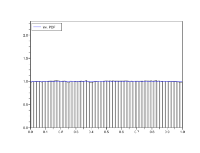
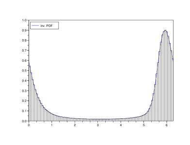
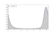
Figure 1:  Left:    theoretical invariant PDF $\,\rho(\theta)\,$ (blue solid line)  compared to the histogram                           of 30000 time values on 1500 trajectories of the processes $\,\theta_{t}$.  In the insert                           the same figure for $\,\tilde{\theta}_{t}\,$ undistinguishable with bare eye from the one for $\,x_{t}$                                  Right: the same figures for the process $\,x_{t}\,$ obtained by the change of variables                          (3.26)

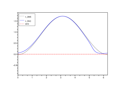
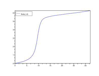
Figure 2: Left:  mean local velocity (blue solid line, everywhere positive) as compared                           to the deterministic velocity equal to the drift term in Eq. (3.23) (black                           dotted line changing sign, with a repulsive and an attractive fixed points                           well visible in the blowups)                                    Right:  Lagrangian trajectory $\,\theta_{L}(t)\,$ of the mean local velocity with $\,\theta_{L}(0)=0$

3.4 Examples

3.4.1 Colloidal particle on a circle

The simplest example of a non-equilibrium Langevin dynamics is provided by the overdamped motion of a particle on a circle with its angular position satisfying the stochastic equation

$$\dot{\theta}_{t}\ =\ -(\partial_{\theta}H)(\theta_{t})\,+\,F\,+\,\zeta_{t}$$ (3.23)

with a periodic potential $\,H(\theta)=H(\theta+2\pi)$,  a constant (non-conservative) force $\,F$,  and a white noise $\,\zeta_{t}\,$ with covariance $\ \langle\zeta_{t}\,\zeta_{s}\rangle=2D\delta(t-s)$.  Eq. (3.23) has a stationary solution with the invariant PDF $\,\rho\,$ given by the formula:

$$\rho(\theta)\ =\ Z^{-1}{\rm e}^{-\frac{1}{D}(H(\theta)-F\theta)}\Big{(}\int\limits_{0}^{\theta}{\rm e}^{\,\frac{1}{D}(H(\vartheta)-F\vartheta)}d\vartheta\,+\,{\rm e}^{\,\frac{2\pi F}{D}}\int\limits_{x}^{2\pi}{\rm e}^{\,\frac{1}{D}(H(\vartheta)-F\vartheta)}d\vartheta\Big{)}\,,$$ (3.24)

where $\,Z\,$ is the normalization factor.  The current corresponding to this density is constant:

$$j\ =\ \big{[}-(\partial_{\theta}H)(\theta)+F-D\partial_{\theta}\big{]}\rho(\theta)\ =\ DZ^{-1}\big{(}{\rm e}^{\,\frac{2\pi F}{D}}-1\big{)}\,.$$ (3.25)

The one-dimensional dynamics becomes simpler in the variable

$$x\ =\ \int\limits_{0}^{\theta}\rho(\vartheta)\,d\vartheta\,.$$ (3.26)

taken modulo $\,1$.  Note that $\,\frac{dx}{d\theta}=\rho(\theta)=jv(\theta)^{-1}\,$ so that $\,j^{-1}x\,$ is the time that the Lagrangian trajectory $\,\theta_{L}(t)\,$ of the mean local velocity starting at $\,\theta=0\,$ takes to get to $\,\theta$. In the variable $\,x$,  the invariant density $\,\rho(x)\equiv 1\,$ and Eq. (3.23) takes the form

$$\dot{x}_{t}\ =\ j\,+\,r(x_{t})\,+\,\zeta_{t}(x_{t})\,,$$ (3.27)

where $\ \zeta_{t}(x)=\rho(\theta)\zeta_{t}\$ for $\ \theta=\theta_{L}(j^{-1}x)\$ and

$$r(x)\ =\ D\rho(\theta)\,\partial_{x}\rho(\theta)\ =\ D(\partial_{\theta}\rho)(\theta)\ =\ \big{[}-(\partial_{\theta}H)(\theta)+F\big{]}\rho(\theta)\,-\,j\,.$$ (3.28)

In the variable $\,x$,  the mean local velocity $\,v(x)\equiv j$.  The corresponding Lagrangian-frame process $\,\tilde{x}_{t}=x_{t}-j(t-t_{0})\,$ and it satisfies the equilibrium-type Langevin equation

$$\dot{\tilde{x}}_{t}\ =\ \tilde{r}_{t}(\tilde{x}_{t})\,+\,\tilde{\zeta}_{t}(\tilde{x}_{t})$$ (3.29)

with $\,\tilde{r}_{t}(\tilde{x})=r(\tilde{x}+j(t-t_{0}))\,$ and $\,\tilde{\zeta}_{t}(\tilde{x})=\zeta_{t}(\tilde{x}+j(t-t_{0}))\,$ and a constant Hamiltonian.

Fig. 1 and Fig. 2 represent the invariant density and the mean local velocity with its Lagrangian trajectory, both for the process $\,\theta_{t}\,$ satisfying Eq. (3.23) with $\,H(\theta)=0.87s^{-1}\times\sin(\theta)$, $\,F=0.85s^{-1}\,$ and $\,D=0.036s^{-1}$.  Such process models the dynamics of a colloidal particle kept by an optical tweezer on a nearly circular orbit in the experiment described in [11].

3.4.2 Linear stochastic equations

A general class of explicitly soluble examples of non-equilibrium dynamics, with multiple applications, is provided by stationary linear SDEs in $d$ dimensions of the form:

$$\dot{x}_{t}\ =\ Mx_{t}\,+\,\zeta_{t}\,,$$ (3.30)

where $\,M\,$ is a matrix whose eigenvalues have negative real part and where

$$\big{\langle}\,\zeta_{t}^{i}\ \zeta_{s}^{j}\,\big{\rangle}\ =\ 2\,D^{ij}\,\delta(t-s)\,,$$ (3.31)

with a positive matrix $\,D=(D^{ij})$.  Here, the invariant density has the Gaussian form [5]

$$\rho(x)\ =\ Z^{-1}{\rm e}^{-\,\beta\,H(x)}$$ (3.32)

with

$$H(x)\ =\ \frac{{}_{1}}{{}^{2\beta}}\,x\cdot C^{-1}x\qquad{\rm for}\qquad C\,=\,2\int\limits_{0}^{\infty}{\rm e}^{tM}D\,{\rm e}^{tM^{T}}\,dt\,.$$ (3.33)

The time-integral in the formula for the covariance $\,C\,$ converges due to the assumption on the eigenvalues of $\,M$.  The mean local velocity corresponding to $\,\rho(x)\,$ is

$$v(x)\ =\ (M\,+\,DC^{-1})\,x$$ (3.34)

so that it depends linearly on $\,x$.  The Lagrangian-frame process

$$\tilde{x}_{t}\ =\ {\rm e}^{-(M+DC^{-1})(t-t_{0})}x_{t}$$ (3.35)

satisfies the time-dependent equilibrium-type linear Langevin equation

$$\dot{\tilde{x}}_{t}\ =\ -\beta\,\tilde{D}_{t}\nabla H(\tilde{x})\,+\,\tilde{\zeta}_{t}$$ (3.36)

where the white noise $\ \tilde{\zeta}_{t}\,=\,{\rm e}^{-(M+DC^{-1})(t-t_{0})}\zeta_{t}\$ has the covariance

$$\big{\langle}\,\tilde{\zeta}_{t}^{i}\,\tilde{\zeta}_{s}^{j}\,\rangle\ =\ 2\,\delta(t-s)\,\tilde{D}^{ij}_{t}\qquad{\rm with}\qquad\tilde{D}_{t}\ =\ {\rm e}^{-(M+DC^{-1})(t-t_{0})}\,D\hskip 2.13387pt{\rm e}^{-(M+DC^{-1})^{T}(t-t_{0})}\,.$$ (3.37)

3.4.3 Sheared suspensions

Stochastic equations of the type (2.1) may be used to model the dynamics of suspensions of colloidal particles [14] or of a polymer, undergoing an overdamped motion driven by conservative forces and opposed by friction, see [29] for a recent discussion. An example is provided by the set of equations for the three-dimensional positions $\,\bm{r}_{i}\,$ of $\,N\,$ particles:

$$\gamma\,\dot{r}^{a}_{i}\,=\,-\,\partial_{r^{a}_{i}}H(\underline{\bm{r}})\,-\,\gamma\,u^{a}_{t}(\bm{r}_{i})\,+\,\zeta^{a}_{i,t}\,,$$ (3.38)

where $\,\gamma\,$ is the friction coefficient, $\ \underline{\bm{r}}=(\bm{r}_{i})_{i=1}^{N}$, $\ H(\underline{\bm{r}})\,$ is the potential energy and $\,\bm{u}(t,\bm{r})\,$ is the velocity field of the solvent. $\,\xi^{a}_{i,t}\,$ are the components of the white noise with the covariance

$$\big{\langle}\,\zeta^{a}_{i,t}\,\zeta^{b}_{j,s}\,\big{\rangle}\ =\ 2\,\gamma\,\beta^{-1}\delta^{ab}\,\delta_{ij}\,\delta(t-s)\,.$$ (3.39)

For a diluted colloidal suspension, assuming only 2-body isotropic interactions, one may take

$$H(\underline{\bm{r}})\ =\ \sum\limits_{i<j}U(r_{ij})\,+\,\sum\limits_{i}U_{0}({\bm{r}}_{i})$$ (3.40)

for $\,r_{ij}\equiv|{\bm{r}}_{i}-{\bm{r}}_{j}|\,$ and for the polymer modeled as a chain of beads with nearest neighbor interaction (Rouse model [27]),

$$H(\underline{\bm{r}})\ =\sum\limits_{i<N}U(r_{i\,(i+1)})\,+\,\sum\limits_{i}U_{0}({\bm{r}}_{i})\,.$$ (3.41)

If the solvent is at rest, and the external potential $\,U_{0}\,$ is confining then the detailed balance holds for the normalized Gibbs density $\,\rho_{0}(\underline{\bm{r}})=Z^{-1}{\rm e}^{-\beta H(\underline{\bm{r}})}\,$ which is left invariant under evolution.  If, however, the solvent undergoes a shear flow with $\,{\bm{u}}_{t}(\bm{r})=f({\bm{r}}\cdot{\bm{e}}_{1})\,{\bm{e}}_{2}$,  where $\,{\bm{e}}_{i}\,$ are the vectors of the canonical basis of $\,{\mathbf{R}}^{3}$,  or a vortical motion with $\,\bm{u}_{t}(\bm{r})=g(|{\bm{r}}\wedge{\bm{e}}_{3}|)\,{\bm{r}}\wedge{\bm{e}}_{3}$,  then the detailed balance is broken and the mean local velocity becomes equal in the stationary state to

$$v^{a}_{i}(\underline{\bm{r}})\ =\ -\,\gamma^{-1}\partial_{r^{a}_{i}}H(\underline{\bm{r}})\,-\,u^{a}_{t}(\bm{r}_{i})\,-\,(\gamma\beta)^{-1}\,\partial_{r^{a}_{i}}\ln\rho(\underline{\bm{r}})\,.$$ (3.42)

where $\,\rho(\underline{\bm{r}})\,$ is the non-Gibbsian invariant density.

In general, the form of $\,\rho(\underline{\bm{r}})\,$ is difficult to access in realistic situations. One of exceptions is the idealized case leading to the linear stochastic equations describing the simplest realization of the Rouse model of a polymer suspension with $\,U(r)=\frac{1}{2}\kappa r^{2}$ and $\,U_{0}(\bm{r})=\frac{1}{2}kr^{2}\,$ and with linear velocity field $\,\bm{u}_{t}(\bm{r})$.  For the vortical velocity $\,\bm{u}_{t}(\bm{r})=\omega\,{\bm{r}}\wedge{\bm{e}_{3}}$,  the stochastic equation (3.38) takes the form (3.30) with

$$M^{ab}_{ij}\,=\,-\gamma^{-1}\delta^{ab}(-\kappa\Delta_{ij}+k\delta_{ij})\,+\,\omega\,\epsilon_{ab3}\,\delta_{ij}\,,$$ (3.43)

where $\,\Delta_{ij}=\sum\limits_{|i^{\prime}-i|=1}(\delta_{i^{\prime}j}-\delta_{ij})$,   and with the matrix

$$D^{ab}_{ij}\,=\,(\gamma\beta)^{-1}\delta^{ab}\,\delta_{ij}\,.$$ (3.44)

in the noise covariance (3.31).  In spite of the vortical motion of the solvent, the Gibbs density $\,\rho_{0}(\underline{\bm{r}})\,$ independent of the vorticity $\,\omega\,$ remains invariant for the symmetry reasons.  Nevertheless, for $\,\omega\not=0$,  the detailed balance is broken and the mean local velocity is given by the solvent velocity

$$v^{a}_{i}(\underline{\bm{r}})\ =\ \omega\,{\bm{r}}_{i}\wedge{\bm{e}_{3}}\,.$$ (3.45)

The Lagrangian frame just rigidly rotates around the third axis with the angular velocity $\,\bm{\Omega}=\omega\,{\bm{e}}_{3}\,$ and the Lagrangian-frame process $\,\tilde{\bm{r}}_{i,t}\,$ satisfies the stochastic equation (3.38) with $\,{\bm{u}}_{t}\,$ set to zero.

Keeping the same harmonic potentials but replacing the vortical solvent motion by the shear flow with $\,u_{t}(\bm{r})\,=\,s\,({\bm{r}}\cdot{\bm{e}}_{1})\,{\bm{e}}_{2}\,$ with a constant shear rate $\,s$,  we obtain the linear stochastic equation (3.30) with

$$M^{ab}_{ij}\ =\ -\gamma^{-1}\delta^{ab}(-\kappa\Delta_{ij}+k\delta_{ij})\,+\,s\,\delta^{a2}\delta^{b1}\,\delta_{ij}$$ (3.46)

and the noise covariance as before.  The $\,N\times N\,$ matrix $\,-\Delta=(-\Delta_{ij})\,$ has the eigenvalues $\,\omega_{k}=2\big{[}1-\cos\big{(}\frac{\pi k}{N}\big{)}\big{]}\,$ corresponding to the normalized eigenvectors

$$(\varphi^{\ell}_{j})\,=\,\big{(}(\frac{{}_{2}}{{}^{N}})^{1/2}\cos\big{(}\frac{{}_{\pi\ell(j-\frac{{}_{1}}{{}^{2}})}}{{}^{N}}\big{)}\big{)}\qquad{\rm for}\qquad\ell=0,1,\dots,N-1\,.$$ (3.47)

The passage to the Fourier modes $\,\hat{\bm{r}}_{\ell}\equiv{\bm{r}}_{j}\varphi_{j}^{\ell}\,$ (sum over $j$) diagonalizes matrix $\,M\,$ into $\,3\times 3\,$ blocs with the entries $\,M^{ab}_{\ell}=\delta^{ab}\mu_{\ell}+s\,\delta^{a2}\delta^{b1}\,$ for $\,\mu_{\ell}\equiv\kappa\omega_{\ell}+k$.  The invariant density $\,\rho(\underline{\bm{r}})\,$ is Gaussian. Its covariance depends quadratically on the shearing rate $\,s\,$ and is composed of the $\,3\times 3\,$ blocs

$$C^{ab}_{\ell}\ =\ \frac{{}_{1}}{{}^{\beta\mu_{\ell}}}\big{[}\delta^{ab}\,+\,\sigma_{\ell}(\delta^{a1}\delta^{2b}+\delta^{a2}\delta^{1b})\,+\,2\sigma_{\ell}^{2}\delta^{a2}\delta^{2b}\big{]},$$ (3.48)

for $\,\sigma_{\ell}\equiv\frac{{\gamma s}}{{2\mu_{\ell}}}=\frac{\gamma s}{2(\kappa\omega_{\ell}+k)}$,  with the blocs of the inverse covariance:

$$(C^{-1})^{ab}_{\ell}\ =\ \beta\mu_{\ell}\Big{[}\delta^{ab}\,+\,\frac{{}_{\sigma_{\ell}^{2}}}{{}^{1+\sigma_{\ell}^{2}}}\,(\delta^{a1}\delta^{1b}-\delta^{a2}\delta^{2b})\,-\,\frac{{}_{\sigma_{\ell}}}{{}^{1+\sigma_{\ell}^{2}}}\,(\delta^{a1}\delta^{2b}+\delta^{a2}\delta^{1b})\Big{]}.$$ (3.49)

The mean local velocity has the Fourier components

$$\hat{v}(\underline{\bm{r}})^{a}_{\ell}\ =\ (M+DC^{-1})^{ab}_{\ell}\,{\hat{r}}^{b}_{\ell}\,,$$ (3.50)

see Eq. (3.34), with

$$(M+DC^{-1})^{ab}_{\ell}\ =\ \frac{{}_{\mu_{\ell}}}{{}^{\gamma}}\Big{[}\frac{{}_{\sigma_{\ell}^{2}}}{{}^{1+\sigma_{\ell}^{2}}}\,(\delta^{a1}\delta^{1b}-\delta^{a2}\delta^{2b})\,-\,\frac{{}_{\sigma_{\ell}}}{{}^{1+\sigma_{\ell}^{2}}}\,(\delta^{a1}\delta^{2b}+\delta^{a2}\delta^{1b})\,+\,2\sigma_{\ell}\delta^{a2}\delta^{1b}\Big{]}$$ (3.51)

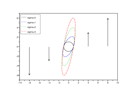
and is incompressible. Its Lagrangian flow is linear. It factorizes for different Fourier modes and takes place along ellipses in the planes orthogonal to $\,{\bm{e}}_{3}$:

$$\hat{\phi}_{t}(\underline{\bm{r}})^{a}_{\ell} = \delta^{a3}\hat{r}^{3}_{\ell}\,+\,(\delta^{a1}\hat{r}^{1}_{\ell}+\delta^{a2}\hat{r}^{2}_{\ell})\,\cos\Big{(}\frac{{}_{s(t-t_{0})}}{{}^{2\sqrt{1+\sigma_{\ell}^{2}}}}\Big{)}\,+\,\Big{[}\,(\delta^{a1}\hat{r}^{1}_{\ell}-\delta^{a2}\hat{r}^{2}_{\ell})\,\frac{{}_{\sigma_{\ell}}}{{}^{\sqrt{1+\sigma_{\ell}^{2}}}}$$ (3.53)

$$-\,(\delta^{a1}\hat{r}^{2}_{\ell}+\delta^{a2}\hat{r}^{1}_{\ell})\,\frac{{}_{1}}{{}^{\sqrt{1+\sigma_{\ell}^{2}}}}\,+\,2\delta^{a2}\hat{r}^{1}_{\ell}\,\sqrt{1+\sigma_{\ell}^{2}}\,\Big{]}\,\sin\Big{(}\frac{{}_{s(t-t_{0})}}{{}^{2\sqrt{1+\sigma_{\ell}}}}\Big{)},$$

see Fig. 3.  The ellipses are more and more elongated in the direction of the flow with increasing shearing rate $\,s\,$ and decreasing Fourier mode $\,\ell$.

Figure 3:   Ellipses followed in the $xy$-plane under the Lagrangian flow of mean local velocity                 by the Fourier modes $\,\hat{\bm{r}}_{\ell}\,$ starting at $\,(1,0)$ for different values of the parameter                 $\sigma_{\ell}=\frac{\gamma s}{4\kappa\big{(}1-cos(\frac{\pi\ell}{N})\big{)}+2k}$

The formula for the time-dependent covariance $\,\tilde{D}_{t}\,$ of the noise in the Lagrangian-frame process is given in Appendix C.

3.5 Back to Eulerian frame

When passing to the Lagrangian frame, a part of the information about the system contained in the probability current or mean local velocity is lost. If we want to reconstruct the original Eulerian process $\,x_{t}$,  we have to supply the forgotten information. A convenient way to do that is to provide the local velocity transformed to the Lagrangian frame:

$$\tilde{v}^{i}_{t}(\tilde{x})\ =\ (\partial_{k}\Phi^{-1}_{t})^{i}(x)\,v^{k}_{t}(x)\ =\ -(\partial_{t}\Phi^{-1}_{t})^{i}(x)$$ (3.54)

for $\,x=\Phi_{t}(\tilde{x})$.  Given the vector field $\,\tilde{v}_{t}(\tilde{x})$,  consider the flow of transformations $\ x\mapsto\tilde{\Phi}_{t}(x)\$ such that

$$\partial_{t}\tilde{\Phi}_{t}(x)\ =\ -\tilde{v}_{t}\big{(}\tilde{\Phi}_{t}(x)\big{)}\,,\qquad\tilde{\Phi}_{t_{0}}(x)\ =\ x\,.$$ (3.55)

The comparison of Eqs. (3.54) and (3.55) shows that $\,\tilde{\Phi}_{t}(x)=\Phi_{t}^{-1}(x)$.  This permits to reconstruct the original process as

$$x_{t}\ =\ \tilde{\Phi}^{-1}_{t}(\tilde{x}_{t})$$ (3.56)

and the original mean local velocity as

$$v^{i}_{t}(x)\ =\ (\partial_{j}\tilde{\Phi}^{-1}_{t})^{i}(\tilde{x})\,\tilde{v}^{j}_{t}(\tilde{x})\ =\ -(\partial_{t}\tilde{\Phi}^{-1}_{t})^{i}(\tilde{x})$$ (3.57)

for $\,\tilde{x}=\tilde{\Phi}_{t}(x)$.  In the special case when the mean local velocity is time-independent (for example when $\,x_{t}\,$ is a stationary process),

$$\tilde{v}^{i}_{t}(\tilde{x})\ =\ -(\partial_{t}\Phi^{-1}_{t})^{i}(x)\ =\ -(\partial_{t}\Phi_{-t})^{i}(x)\ =\ v^{i}\big{(}\Phi_{-t})^{i}(x)\big{)}\ =\ v^{i}(\tilde{x})$$ (3.58)

so that the velocity field $\,\tilde{v}_{t}\,$ coincides with the mean local velocity of the Eulerian frame and is time-independent.

As we see, the knowledge of the non-equilibrium diffusion $\,x_{t}\,$ is equivalent to the knowledge of the equilbrium diffusion $\,\tilde{x}_{t}\,$ and of the (deterministic) velocity field $\,\tilde{v}_{t}$.

4 Diffusion Processes with Hamiltonian forces

4.1 Modified probability current and mean local velocity

In many applications, one deals with non-equilibrium diffusions in the presence of Hamiltonian forces. It is then useful to single out their contribution and to replace the SDE (2.1) by

$$\dot{x}_{t}^{i} = \,u^{i}_{t}(x)\,+\,\Pi^{ij}_{t}(x_{t})\,(\partial_{j}H)(x_{t})\,-\,\beta^{-1}\,(\partial_{j}\Pi^{ij}_{t})(x_{t})\,+\,\zeta^{i}_{t}(x_{t})$$ (4.1)

where the term $\,\Pi^{ij}_{t}\,\partial_{j}H_{t}\,$ with $\,\Pi_{t}^{ij}=-\Pi_{t}^{ji}\,$ stands for the Hamiltonian force. Geometrically, the antisymmetic tensor field $\,\Pi_{t}^{ij}\,$ represents a (possibly time dependent) Poisson structure but we shall not need its property that assures the Jacobi identity of the Poisson bracket. The subtraction of $\,\beta^{-1}\partial_{j}\Pi^{ij}_{t}\,$ on the right hand side of Eq. (4.1) assures that the terms involving $\,\Pi_{t}\,$ transform as a vector field under a change of coordinates if the Gibbs factor $\,{\rm e}^{-\beta H}\,$ transforms as a density.  An example of dynamics (4.1) is provided by the Langevin equation

$$\dot{x}_{t}^{i} = -\,\beta\,d^{ij}_{t}(x_{t})\,(\partial_{j}H_{t})(x_{t})\,+\,r^{i}_{t}(x_{t})\,+\,F^{i}_{t}(x_{t})$$ (4.4)

$$+\,\Pi^{ij}_{t}(x_{t})\,(\partial_{j}H)(x_{t})\,-\,\beta^{-1}\,(\partial_{j}\Pi^{ij}_{t})(x_{t})\,+\,\zeta^{i}_{t}(x_{t})\,,$$

compare to Eq. (3.22).  In the presence of Hamiltonian forces, it is convenient to redefine the probability current as

$$j^{i}_{t}\ =\ \big{[}\hat{u}^{i}_{t}\,+\,\Pi^{ij}_{t}(\partial_{j}H_{t})\,-\,b^{ij}_{t}\,\partial_{j}\big{]}\hskip 0.85355pt\rho_{t}\,,$$ (4.5)

where $\,b^{ij}_{t}=d^{ij}_{t}-\beta^{-1}\Pi^{ij}_{t}$.  The new expression for the current $\,j_{t}\,$ differs from the one prescribed by Eq. (2.10) by the addition of the term $\ \beta^{-1}\partial_{j}\big{(}\Pi^{ij}_{t}\rho_{t})$.  The continuity equation (2.9) still holds since the added term is divergence-less so that the flux of $\,j_{t}\,$ through the boundary of any region $\,{\cal V}\,$ still gives the rate of change of the probability that $\,x_{t}\,$ belongs to $\,{\cal V}$.  For the case of the Langevin equation (4.4), the new expression for the current reduces to

$$j^{i}_{t}\ =\ \big{[}-\beta\,b^{ij}_{t}\,\partial_{j}H_{t}\,+\,F^{i}_{t}\,-\,b^{ij}_{t}\,\partial_{j}\big{]}\hskip 0.85355pt\rho_{t}\,.$$ (4.6)

In particular, if $\,H_{t}\equiv H\,$ is time-independent and the additional force $\,F_{t}\equiv 0\,$ then the modified probability current (4.6) associated to the Gibbs density $\,\rho(x)=Z^{-1}{\rm e}^{-\beta\,H(x)}\,$ vanishes and $\,\rho\,$ is preserved by the evolution. It is then natural to extend the notion of equilibrium dynamics to such a case.

As before, we may introduce the velocity field by the relation

$$v^{i}_{t}\ =\ \rho_{t}^{-1}j^{i}_{t}\ =\ \hat{u}^{i}_{t}\,+\,\Pi^{ij}_{t}(\partial_{j}H_{t})\,-\,b^{ij}_{t}\,\partial_{j}\ln{\rho_{t}}\,.$$ (4.7)

Since now

$$v^{i}_{t}(x)\ =\ \frac{\big{\langle}\,\dot{x}_{t}\,\,\delta(x-x_{t})\,\big{\rangle}}{\big{\langle}\,\delta(x-x_{t})\,\big{\rangle}}\ +\ \beta^{-1}\rho_{t}(x)^{-1}\partial_{j}\big{(}\Pi^{ij}_{t}\rho_{t}\big{)}(x)\,,$$ (4.8)

we shall call $\,v_{t}(x)\,$ the subtracted mean local velocity. The continuity equation (2.9) still takes the form of the advection equation (2.13).

If we realize the passage to the Lagrangian frame of the velocity $\,v_{t}\,$ of Eq. (4.7) as described in Sect. 3.1, using the flow of $\,v_{t}\,$ that we shall still denote by $\,\Phi_{t}\,$ and introducing the Lagrangian-frame process $\,\tilde{x}_{t}=\Phi_{t}^{-1}(x_{t})$, then the considerations of Sect. 3.2 go unchanged because they only use the advection equation (2.9), not the explicit form of $\,v_{t}(x)$.  As before, we infer that the instantaneous PDF of the process $\,\tilde{x}_{t}\,$ is frozen to the time $\,t_{0}\,$ value $\,\rho_{t_{0}}\,$ of the PDF of the Eulerian process $\,x_{t}$.

On the other hand, in the derivation of the SDE for the Lagrangian-frame process in Sect. 3.3, the explicit form of $\,v_{t}(x)\,$ was used in Eq. (3.10).  As a consequence, the SDE for $\,\dot{\tilde{x}}^{i}_{t}\,$ will pick now the additional term

$$-(\partial_{k}\Phi^{-1}_{t})^{i}(x_{t})\,\beta^{-1}\rho_{t}(x)^{-1}\partial_{l}\big{(}\Pi^{kl}_{t}\,\rho_{t}\big{)}(x_{t})$$ (4.9)

(4.10)

$$=\ -\beta^{-1}(\partial_{k}\Phi^{-1}_{t})^{i}(x_{t})\,\big{[}\Pi^{kl}_{t}(x_{t})\,(\partial_{l}\ln{\rho_{t}})(x_{t})\,+\,(\partial_{l}\Pi^{kl}_{t})(x_{t})\big{]}$$ (4.11)

(4.12)

$$=\ -\beta^{-1}(\partial_{k}\Phi^{-1}_{t})^{i}(x_{t})\,\big{[}\Pi^{kl}_{t}(x_{t})\,(\partial_{l}\Phi^{-1}_{t})^{j}(x_{t})\,(\partial_{j}\rho_{t_{0}})(\tilde{x}_{t})$$ (4.13)

(4.14)

$$\hskip 65.44142pt+\,\Pi^{kl}_{t}(x_{t})\,(\partial_{j}\Phi_{t})^{h}(\tilde{x}_{t})\,(\partial_{l}\partial_{h}\Phi_{t}^{-1})^{j}(x_{t})\,+\,(\partial_{l}\Pi^{kl}_{t})(x_{t})\big{]}\,,$$ (4.15)

where the second equality follows from Eq. (3.18) and the identity $\,\tilde{\rho}_{t}=\rho_{t_{0}}$.  Introducing the Lagrangian-frame antisymmetric tensor field

$$\tilde{\Pi}^{ij}_{t}(\tilde{x})\ =\ (\partial_{k}\Phi^{-1}_{t})^{i}(x)\,\Pi^{kl}_{t}(x)\,(\partial_{l}\Phi^{-1}_{t})^{j}(x)$$ (4.16)

where $\,x=\Phi_{t}(\tilde{x})\,$ and observing that

$$(\partial_{j}\tilde{\Pi}^{ij}_{t})(\tilde{x}) = \big{[}(\partial_{h}\partial_{k}\Phi^{-1}_{t})^{i}(x)\,\Pi^{kl}_{t}(x)\,(\partial_{l}\Phi^{-1}_{t})^{j}(x)\,+\,(\partial_{k}\Phi^{-1}_{t})^{i}(x)\,(\partial_{h}\Pi^{kl}_{t})(x)\,(\partial_{l}\Phi^{-1}_{t})^{j}(x)$$ (4.19)

$$\hskip 113.81102pt+\,(\partial_{k}\Phi^{-1}_{t})^{i}(x)\,\Pi^{kl}_{t}(x)\,(\partial_{h}\partial_{l}\Phi^{-1}_{t})^{j}(x)\big{]}\,(\partial_{j}\Phi_{t})^{h}(\tilde{x})$$

$$= (\partial_{k}\Phi^{-1}_{t})^{i}(x)\,(\partial_{l}\Pi^{kl}_{t})(x)\,+\,(\partial_{k}\Phi^{-1}_{t})^{i}(x)\,\Pi^{kl}_{t}(x)\,(\partial_{h}\partial_{l}\Phi^{-1}_{t})^{j}(x)\,(\partial_{j}\Phi_{t})^{h}(\tilde{x})\,,$$ (4.21)

we may rewrite the additional term (4.15) as

$$-\beta^{-1}\tilde{\Pi}^{ij}_{t}(\tilde{x}_{t})\,(\partial_{j}\rho_{t_{0}})(\tilde{x}_{t})\,-\,\beta^{-1}(\partial_{j}\tilde{\Pi}^{ij}_{t})(\tilde{x}_{t})\ =\ \tilde{\Pi}^{ij}_{t}(\tilde{x}_{t})\,\partial_{j}\tilde{H}(\tilde{x}_{t})\,-\,\beta^{-1}(\partial_{j}\tilde{\Pi}^{ij}_{t})(\tilde{x}_{t})\,.$$ (4.22)

Altogether, the Lagrangian-frame process $\,\tilde{x}_{t}\,$ satisfies now the equilibrium-type time-dependent SDE with a Hamiltonian force:

$$\dot{\tilde{x}}^{i}_{t}\ =\ -\beta\,\tilde{d}^{ij}_{t}(\tilde{x}_{t})\,(\partial_{j}\tilde{H})(\tilde{x}_{t})\,dt\,+\,\tilde{\Pi}^{ij}_{t}(\tilde{x}_{t})\,(\partial_{j}\tilde{H})(\tilde{x}_{t})\,-\,\beta^{-1}(\partial_{j}\tilde{\Pi}^{ij}_{t})(\tilde{x}_{t})\,+\,\tilde{r}^{i}_{t}(\tilde{x}_{t})\,+\,\tilde{\zeta}^{i}_{t}(\tilde{x}_{t})\,,$$ (4.23)

Clearly, the modified probability current associated with the conserved density $\,\rho_{t_{0}}=\tilde{Z}^{-1}{\rm e}^{-\beta\,\tilde{H}}\,$ vanishes for the Lagrangian-frame process.

4.2 Example of Langevin-Kramers dynamics

The particular case of Langevin dynamics with Hamiltonian forces is provided by the $2^{\rm nd}$ order Langevin-Kramers SDE

$$m_{ij}\,\ddot{q}^{j}_{t}\ =\ -\,\gamma_{ij}\,\dot{q}_{t}^{j}\,-\,\partial_{i}V_{t}(q_{t})\,+\,f_{i}(q_{t})\,+\,\xi_{t,i}$$ (4.24)

with the positive mass $\,m=(m_{ij})$ and friction $\,\gamma=(\gamma_{ij})\,$ matrices that, for simplicity, we assume independent of $\,t\,$ and $\,q$,  with a potential $\,V_{t}(q)$ and a non-conservative force $\,f_{t}(q)$,  and with a white noise $\,\xi_{t}\,$ with the covariance

$$\langle\,\xi_{t,i}\,\xi_{s,j}\,\rangle\ =\ 2\,\beta^{-1}\sigma_{ij}\,\delta(t-s)\,.$$ (4.25)

We keep the matrix $\,\sigma\,$ different from $\,\gamma\,$ to allow noises modeling environments with variable temperature that violate the Einstein relation $\,\sigma=\gamma$.  The $2^{\rm nd}$ order equation (4.24) may be rewritten as the $1^{\rm st}$ order SDE (4.4) in the phase space of points $\,x=(q,p)\,$ if we set

$$d\,=\,\Big{(}\begin{matrix}{}_{0}&{}_{0}\cr{}^{0}&{}^{\beta^{-1}\sigma}\end{matrix}\Big{)}\,,\qquad\Pi\,=\,\Big{(}\begin{matrix}{}_{0}&{}_{1}\cr{}^{-1}&{}^{0}\end{matrix}\Big{)}\,,\qquad H_{t}\,=\,\frac{{}_{1}}{{}^{2}}\,p\cdot m^{-1}p\,+\,V_{t}(q)\,,$$ (4.26)

$$F_{t}\,=\,(0,\,(\sigma-\gamma)m^{-1}p+f_{t}(q)),,\qquad\zeta_{t}=(0,\,\xi_{t})\,.$$

The subtracted mean local velocity in the phase space has here the form

$$v_{t}\ =\ \big{(}m^{-1}p+\beta^{-1}\nabla_{p}\ln{\rho_{t}}\,,\ -\nabla V_{t}-\gamma\,m^{-1}p+f_{t}-\beta^{-1}\nabla_{q}\ln{\rho_{t}}-\beta^{-1}\sigma\,\nabla_{p}\ln{\rho_{t}}\big{)}$$ (4.27)

and it vanishes for the Gibbs density $\ \rho(q,p)=Z^{-1}{\rm e}^{-\beta\,H(q,p)}\$ in the equilibrium case where $\,\sigma=\gamma$,  the potential $\,V_{t}\,$ is time-independent, and the non-conservative force $f_{t}\,$ is absent.

4.2.1 Harmonic chain

An example of a Langevin-Kramers dynamics is provided by a Fermi-Pasta-Ulam chain [9] with ends coupled to a friction force and a white noise. Such chains were often used in the theoretical studies of the Fourier law [2].  Here $\,q=(r^{a}_{i})\,$ with $\,i=1,\dots,N$, $a=1,\dots,d$,  and

$$\gamma^{ab}_{ij}\,=\,\gamma_{0}\,\delta^{ab}(\delta_{i1}\delta_{1j}+\delta_{iN}\delta_{Nj})\,,\qquad\sigma^{ab}_{ij}\,=\,\gamma_{0}\,\delta^{ab}\big{(}(1+\eta)\delta_{i1}\delta_{1j}+(1-\eta)\delta_{iN}\delta_{Nj}\big{)}\,,$$ (4.28)

$$m^{ab}_{ij}\,=\,m_{0}\,\delta^{ab}\,\delta_{ij}\,,\qquad V(q)\,=\,\sum\limits_{i<N}^{N}U(r_{i\,(i+1)})\,+\,\sum\limits_{i}U_{0}(\bm{r}_{i})\,,$$ (4.29)

The dynamics in the bulk (i.e. for $\,i\not=1,N$)  is purely Hamiltonian, whereas the boundary degrees of freedom $\,\bm{r}_{0}\,$ and $\,\bm{r}_{N}\,$ are exposed to the thermal noise at temperatures $\,\beta^{-1}(1\pm\eta)$,  respectively, and to friction.  The harmonic case (that does not lead to the Fourier law [25]) with $\,U(r)=\frac{\kappa}{2}r^{2}\,$ and $\,U_{0}(\bm{r})=\frac{k}{2}r^{2}\,$ corresponds to the linear stochastic equation of the type (3.30) with the matrices

$$M^{ab}_{ij}\ =\ \delta^{ab}\,\Big{(}\begin{matrix}{}_{0}&{}_{m_{0}^{-1}\delta_{ij}}\cr{}^{-(-\kappa\Delta+k)_{ij}}&{}^{-\gamma_{0}m_{0}^{-1}(\delta_{i1}\delta_{1j}+\delta_{iN}\delta_{Nj})}\end{matrix}\Big{)}\,,$$ (4.30)

$$D^{ab}_{ij}\ =\ \beta^{-1}\gamma_{0}\,\delta^{ab}\,\Big{(}\begin{matrix}{}_{0}&{}_{0}\cr{}^{0}&{}^{(1+\eta)\delta_{i1}\delta_{1j}+(1-\eta)\delta_{iN}\delta_{Nj}}\end{matrix}\Big{)}\,.$$ (4.31)

The covariance matrix of the invariant Gaussian measure has the form

$$C^{ab}_{ij}\ =\ \beta^{-1}\delta^{ab}\,\Big{(}\begin{matrix}{}_{\big{(}\frac{1}{-\kappa\Delta+k}\big{)}_{ij}}&{}_{0}\cr{}^{0}&{}^{m_{0}\delta_{ij}}\end{matrix}\Big{)}+\beta^{-1}\eta\,\delta^{ab}\,\Big{(}\begin{matrix}{}_{X_{ij}}&{}_{Z_{ij}}\cr{}^{-Z_{ij}}&{}^{Y_{ij}}\end{matrix}\Big{)}$$ (4.32)

with matrices $\,X,Y,Z\,$ that may be calculated exactly [25]  (for $\,\eta=0$,  it reduces to the covariance of the Gibbs measure).  The subtracted mean local velocity is

$$v(q,p)\ =\ \big{(}M+DC^{-1}-\beta^{-1}\Pi C^{-1}\big{)}\,\Big{(}\begin{matrix}{}q\cr{}p\end{matrix}\Big{)},$$ (4.33)

where the matrix on the right hand side has, up to terms quadratic in the relative temperature difference $\,\eta$,  the entries

$$\eta\,m_{0}^{-1}\delta^{ab}\,\Big{(}\begin{matrix}{}_{-\big{(}Z(-\kappa\Delta+k)\big{)}_{ij}}&{}_{m_{0}^{-1}Y_{ij}}\cr{}^{-\big{(}Y(-\kappa\Delta+k)\big{)}_{ij}}&{}^{-\big{(}(-\kappa\Delta+k)Z\big{)}_{ij}-\gamma_{0}m_{0}^{-1}(\delta_{i1}Y_{1j}+\delta_{iN}Y_{Nj})+\gamma_{0}(\delta_{i1}\delta_{1j}-\delta_{iN}\delta_{Nj})}\end{matrix}\Big{)}.$$ (4.34)

The Lagrangian flow of $\,v\,$ is obtained by the linear action of the matrix $\ {\rm e}^{(M+DC^{-1}-\beta^{-1}\Pi C^{-1})(t-t_{0})}\$ which is straightforward to calculate in the linear order in $\,\eta$.

5 Fluctuation-dissipation relations

5.1 Equilibrium Fluctuation-Dissipation Theorem

The equilibrium Fluctuation-Dissipation Theorem [23, 4, 19] relates the spontaneous dynamical fluctuations in an equilibrium state to the relaxation dynamics after a tiny perturbation out of the equilibrium. It holds for a wide class of equilibrium systems including the ones described by the equilibrium Langevin equation

$$\dot{x}_{t}^{i} = -\,\beta\,d^{ij}_{t}(x_{t})\,(\partial_{j}H)(x_{t})\,+\,\pi^{ij}_{t}(x_{t})\,(\partial_{j}H)(x_{t})\,-\,\beta^{-1}\,(\partial_{j}\pi^{ij}_{t})(x_{t})\,+\,r^{i}_{t}(x_{t})\,\,+\,\zeta^{i}_{t}(x_{t})$$ (5.1)

of the type discussed above. We assume that the process $\,x_{t}\,$ has the time-independent Gibbs instantaneous PDF $\,\rho(x)=Z^{-1}{\rm e}^{-\beta\,H(x)}\,$ and denote by $\,\big{\langle}\,-\,\big{\rangle}\,$ the dynamical expectation.  The FDT asserts that [20]

$$\partial_{s}\hskip 0.71114pt\big{\langle}\,O^{1}(x_{s})\,O^{2}(x_{t})\,\big{\rangle}\ =\ \beta^{-1}\frac{{}_{\delta}}{{}^{\delta h_{s}}}\big{|}_{h=0}\,\big{\langle}\,O^{2}(x_{t})\,\big{\rangle}_{h}$$ (5.2)

for $\,s<t$,  where $\,O^{a}(x)\,$ are functions (well behaved at infinity), that we shall call (single-time) observables, and where on the right hand side the expectation $\,\big{\langle}\,-\,\big{\rangle}_{h}\,$ involves the process obtained by replacing the Hamiltonian $\,H(x)\,$ in the original dynamics (5.1) by its time-dependent perturbation $\,H(x)-h_{t}\,O^{1}(x)\,$ within some time interval.  The left hand side is the time derivative of the 2-time correlation function in the dynamics determined by Eq. (5.1) and the right hand side is the response of the single-time correlation function to a small dynamical perturbation of the Hamiltonian of the system. The temperature $\,\beta^{-1}\,$ appears as the coefficient relating the two functions. For the sake of completeness, we give a proof of the FDT (5.2) in Appendix D.  It is often more convenient to consider the time-integrated version of the FDT:

$$\big{\langle}\,O^{1}(x_{t})\,O^{2}(x_{t})\,\rangle\,-\,\big{\langle}\,O^{1}(x_{s})\,O^{2}(x_{t})\,\rangle\ =\ \beta^{-1}\frac{{}_{\partial}}{{}^{\partial h_{0}}}\big{|}_{h_{0}=0}\,\big{\langle}\,O^{2}(x_{t})\,\big{\rangle}_{h_{0},s}\,,$$ (5.3)

where $\,\big{\langle}\,-\,\big{\rangle}_{h_{0},s}\,$ corresponds to the expectation where the original Hamiltonian $\,H(x)\,$ is replaced starting at time $\,s<t\,$ by its time-independent perturbation $\,H(x)-h_{0}O^{1}(x)$.

5.2 Modified Fluctuation Dissipation Theorem

We may immediately apply the FDT to the Lagrangian-frame process $\,\tilde{x}_{t}\,$ obtained from the process $\,x_{t}\,$ satisfying the Langevin equation (4.4).  Indeed, as was shown in Sect. 4.1, the process $\,\tilde{x}_{t}=\Phi_{t}^{-1}(x_{t})$,  where $\,\Phi_{t}\,$ is the flow of the subtracted mean local velocity (4.7),  satisfies the equilibrium stochastic equation (4.23) and has the time-independent instantaneous PDF $\,\rho_{t_{0}}(\tilde{x})=Z^{-1}{\rm e}^{-\beta\,\tilde{H}(\tilde{x})}$.  We infer that for observables $\,\tilde{O}^{a}(\tilde{x})$,

$$\partial_{s}\hskip 0.71114pt\big{\langle}\,\tilde{O}^{1}(\tilde{x}_{s})\,\tilde{O}^{2}(\tilde{x}_{t})\,\rangle\ =\ \beta^{-1}\frac{{}_{\delta}}{{}^{\delta\tilde{h}_{s}}}\big{|}_{\tilde{h}=0}\,\big{\langle}\,\tilde{O}^{2}(\tilde{x}_{t})\,\big{\rangle}_{\tilde{h}}$$ (5.4)

where $\,\big{\langle}\,-\,\big{\rangle}_{\tilde{h}}\,$ involves the process obtained by replacing the Hamiltonian $\,\tilde{H}(\tilde{x})\,$ in the Lagrangian-frame dynamics (4.23) by its time-dependent perturbation $\,\tilde{H}(\tilde{x})-\tilde{h}_{t}\tilde{O}^{1}(\tilde{x})$ during a time interval.  Observe that this perturbation corresponds to the replacement of the Hamiltonian $\,H_{t}(x)\,$ in the original equation (4.4) for $\,x_{t}\,$ by $\,H_{t}(x)-\tilde{h}_{t}\tilde{O}^{1}(\Phi_{t}^{-1}(x))$.  Indeed, the latter replacement adds the term

$$\beta\,\tilde{h}_{t}\,b^{ij}_{t}(x_{t})\,\partial_{x^{j}}\tilde{O}^{1}(\Phi_{t}^{-1}(x))|_{x=x_{t}}$$ (5.5)

on the right hand side of Eq. (4.4) and, in virtue of Eq. (3.9), results in the additional term

$$(\partial_{k}\Phi_{t}^{-1})^{i}(x_{t})\,\Big{[}\beta\,\tilde{h}_{t}\,b^{kl}_{t}(x_{t})\,\partial_{x^{l}}|_{x=x_{t}}\tilde{O}^{1}(\Phi_{t}^{-1}(x))\Big{]}$$ (5.6)

(5.7)

$$=\ \beta\,\tilde{h}_{t}\,(\partial_{k}\Phi_{t}^{-1})^{i}(x_{t})\,b^{kl}_{t}(x_{t})\,(\partial_{l}\Phi_{t}^{-1})^{j}(x_{t})\,(\partial_{j}\tilde{O}^{1})(\tilde{x}_{t})$$ (5.8)

(5.9)

$$=\ \beta\,\tilde{h}_{t}\,\tilde{b}^{ij}_{t}(\tilde{x}_{t})\,(\partial_{j}\tilde{O}^{1})(\tilde{x}_{t})$$ (5.10)

with $\ \tilde{b}^{ij}_{t}=\tilde{d}^{ij}_{t}-\beta^{-1}\tilde{\Pi}^{ij}_{t}\,$ in Eq. (4.23) for $\,\tilde{x}_{t}=\Phi_{t}^{-1}(x_{t})\,$ (with the same transformations $\,\Phi_{t}\,$ as in the unperturbed process).  Upon defining the Eulerian-frame time-dependent observables

$$O^{a}_{t}(x)\ =\ \tilde{O}^{a}(\Phi_{t}^{-1}(x))\,,$$ (5.11)

the Lagrangian-frame FDT (5.4) may be rewritten as the identity

$$\partial_{s}\hskip 0.71114pt\big{\langle}\,O^{1}_{s}(x_{s})\,O^{2}_{t}(x_{t})\,\rangle\ =\ \beta^{-1}\frac{{}_{\delta}}{{}^{\delta\tilde{h}_{s}}}\big{|}_{\tilde{h}=0}\,\big{\langle}\,O^{2}_{t}(x_{t})\,\big{\rangle}_{\tilde{h}}\,.$$ (5.12)

Note that the time-dependent observables $\,O^{a}_{t}(x)\,$ are constant along the Lagrangian trajectories of the velocity (4.7): $\,O^{a}_{t}(\Phi_{t}(x))=\tilde{O}^{a}(x)$.  In other words, they obey the scalar advection equation

$$\partial_{t}O^{a}_{t}\,+\,v_{t}\cdot\nabla O^{a}_{t}\,=\,0\,$$ (5.13)

and are frozen in the Lagrangian frame of the subtracted mean local velocity $\,v_{t}$.  Since the values of the time-dependent observable $\,O^{1}\,$ may be chosen arbitrarily at time $\,s\,$ and that of $\,O^{2}\,$ at time $\,t$,  the only trace of time dependence of the observables $\,O^{a}\,$ in the identity (5.12) for fixed pair of times $\,s<t\,$ enters through the time derivative $\,\partial_{s}\,$ on the left hand side that differentiates also the explicit time-dependence of $\,O^{1}\,$ determined by Eq. (5.13).  We may then rewrite Eq. (5.12) using observables frozen in the Eulerian frame as the Modified Fluctuation-Dissipation Theorem,

$$\partial_{s}\hskip 0.71114pt\big{\langle}\,O^{1}(x_{s})\,O^{2}(x_{t})\,\big{\rangle}\ -\ \big{\langle}\,(v_{s}\cdot\nabla O^{1})(x_{s})\,O^{2}(x_{t})\,\big{\rangle}=\ \beta^{-1}\frac{{}_{\delta}}{{}^{\delta h_{s}}}\big{|}_{h=0}\,\big{\langle}\,O^{2}_{t}(x_{t})\,\big{\rangle}_{h}\,,$$ (5.14)

where the expectation $\,\big{\langle}\,-\,\big{\rangle}_{h}\,$ on the right hand side refers now to the process obtained by replacing the Hamiltonian $\,H_{t}\,$ in Eq. (4.4) by $\,H_{t}(x)-h_{t}\,O^{1}(x)$.  In the time-integrated form, Eq. (5.14) becomes

$$\big{\langle}\,O^{1}(x_{t})\,O^{2}(x_{t})\,\rangle\,-\,\big{\langle}\,O^{1}(x_{s})\,O^{2}(x_{t})\,\rangle\ -\ \int\limits_{s}^{t}\big{\langle}\,(v_{\sigma}\cdot\nabla O^{1})(x_{\sigma})\,O^{2}(x_{t})\,\big{\rangle}\,d\sigma\,\,$$ (5.15)

(5.16)

$$=\ \beta^{-1}\frac{{}_{\partial}}{{}^{\partial h}}\big{|}_{h_{0}=0}\,\big{\langle}\,O^{2}(x_{t})\,\big{\rangle}_{h_{0},s}\,,$$ (5.17)

with a corrective integral term with respect to Eq. (5.3).  An experimental check of the time-integrated MFDT for a colloidal particle has been described in [11]. Fig. 4 shows the numerical check of this relation and of its Lagrangian-frame counterpart for the stationary process solving the SDE (3.23) for $\,O^{a}(\theta)=sin(\theta)$.

Figure 4:  Left:    the bottom coinciding curves: LHS (continuous black) and RHS (dashed red)                          of the integrated MFDT (5.17) for $\,O^{a}(\theta)=\sin(\theta)$, the upper (dot-dashed                          green) curve: the first two terms on its LHS, the middle (dashed blue)                          curve: the corrective integral term                                Right:  RHS (dashed red curve) and LHS (continuous black curve) of the integrated-                          in-time Lagrangian-frame FDT (5.4)  with $\,\tilde{O}^{a}(\tilde{\theta})=\sin(\tilde{\theta})$

The MFDT was proven directly in [6] in the stationary setup and shown to be equivalent to identity (5.12) similar to the equilibrium FDT (5.2) but for observables frozen in the Lagrangian frame of mean local velocity. In the present paper, we unravel the deeper reason for that equivalence, namely the fact that the non-equilibrium diffusion process observed in the Lagrangian frame of the (subtracted) mean local velocity evolves according to an equilibrium dynamics with a time-independent instantaneous PDF.

5.3 Links with fluctuation relations

Ref. [6]) also discussed fluctuation relation extending the MFDT to non-stationary situations. It was shown there that the Hatano-Sasa version [13] of the Jarzynski equality [15, 16] reduces close to stationarity to the MFDT for special observables and that one need Croooks’ extention [7] of the Jarzynski-Hatano-Sasa equality to extract at stationarity the MFDT for general observables. The results of the present paper permit to propose yet another extension of the MFDT.

For the process $\,x_{t}\,$ evolving accordingly to the Langevin equation (2.14) but with a time-dependent Hamiltonian $\,H_{t}(x)$,  the Jarzynski equality reads

$$\big{\langle}\,{\rm e}^{-\beta\,W_{t_{0},t}}\,\big{\rangle}\ =\ \frac{{Z_{t}}}{{Z_{t_{0}}}}\,,$$ (5.18)

where

$$W_{t_{0},t}\ =\ \int\limits_{t_{0}}^{t}(\partial_{s}H)(x_{s})\,ds\,\qquad{\rm and}\qquad Z_{t}=\ \int{\rm e}^{-\beta\,H_{t}(x)}\,dx\,,$$ (5.19)

provided that the PDF of $\,x_{t_{0}}\,$ is $\,Z_{t_{0}}^{-1}{\rm e}^{-\beta H_{t_{0}}}$.  Applied to case with the Hamiltonian $\,H_{t}(x)=H(x)-\sum\limits_{a=1,2}h^{a}_{t}\,O^{a}(x)\,$ and expanded to the second order in functions $\,h^{a}_{t}$,  Eq. (5.18) reduces to the FDT (5.2). The proof goes as in [5] where it was written for a less general case.

The above observations apply to the case of the Lagrangian-frame dynamics. For the process $\,\tilde{x}_{t}\,$ satisfying the SDE (4.23) but with the Hamiltonian $\,\tilde{H}\,$ replaced by $\,\tilde{H}(\tilde{x})+\tilde{H}^{\prime}_{t}(\tilde{x})\,$ with $\,\tilde{H}^{\prime}_{t}=0\,$ for $\,t\leq t_{0}$,  we have for $\,t>t_{0}\,$ the Lagrangian-frame version of the Jarzynski equality:

$$\big{\langle}\,{\rm e}^{-\beta\,\tilde{W}_{t_{0},t}}\,\big{\rangle}\ =\ \frac{\tilde{Z}_{t}}{\tilde{Z}}\qquad{\rm for}\qquad\tilde{W}_{t_{0},t}\ =\ \int\limits_{t_{0}}^{t}(\partial_{s}\tilde{H}^{\prime}_{s})(\tilde{x}_{s})\,ds$$ (5.20)

and $\ \tilde{Z}_{t}=\int\limits{\rm e}^{-\beta\,(\tilde{H}+\tilde{H}^{\prime}_{t})(\tilde{x})}d\tilde{x}$,  provided that the PDF of $\,\tilde{x}_{t_{0}}\,$ is $\,\tilde{Z}^{-1}{\rm e}^{-\beta\,\tilde{H}}=\rho_{t_{0}}$.  The process $\,x_{t}\,$ such that $\,\tilde{x}_{t}=\Phi_{t}^{-1}(x_{t})$,  with $\,\Phi_{t}\,$ standing for the Lagrangian flow of the mean local velocity $\,v_{t}(x)\,$ of the unperturbed process $\,x_{t}$,  satisfies the SDE (4.4) with the original Hamiltonian $\,H_{t}(x)\,$ replaced by $\,H_{t}(x)+H^{\prime}_{t}(\Phi_{t}^{-1}(x))$.  This follows by the same argument as around Eqs. (5.5) and (5.10).  In terms of the perturbed process $\,x_{t}$,

$$\tilde{W}_{t_{0},t}\ =\ \int\limits_{t_{0}}^{t}(\partial_{s}\tilde{H}^{\prime}_{s})\big{(}\Phi_{t}^{-1}(x_{s})\big{)}\,ds\qquad{\rm and}\qquad\frac{\tilde{Z}_{t}}{\tilde{Z}}\ =\ \int{\rm e}^{-\beta\,H^{\prime}_{t}(x)}\rho_{t_{0}}(x)\,dx\,.$$ (5.21)

For $\ \tilde{H}^{\prime}(\tilde{x})=-\sum\limits_{a=1,2}h^{a}_{t}\,\tilde{O}^{a}(\tilde{x})$,  one obtains the Lagrangian-frame FDT (5.4) equivalent to the MFDT (5.14) by expanding the identity (5.20) to the 2^nd order in $\,h^{a}_{t}$.  Not very surprisingly, there exist different fluctuation relations that may be viewed as an extension of the MFDT to more general situations.

6 Non-equilibrium diffusions without Lagrangian picture

In the preceding sections, we have discussed diffusion processes in a finite dimensional phase space. The basic assumption underlying the discussion of the Lagrangian-frame picture of diffusions was the existence of the Lagrangian flow $\,x\mapsto\Phi_{t}(x)\,$ of the mean local velocity satisfying Eqs. (3.2). This is guaranteed if the velocity $\,v_{t}(x)\,$ is smooth and the (phase-)space $\,{\cal X}\,$ is compact, like in the circle example, but may be not assured if $\,{\cal X}\,$ is unbounded in which case the Lagrangian trajectories of $\,v_{t}\,$ may blow up in finite time. The idea of the decoupling of probability flux by the passage to the Lagrangian frame of the mean local velocity can, in principal, be applied to infinite-dimensional diffusive processes. It appears, however, that a number of known examples of diffusive processes described by stochastic PDEs do not allow a global flow of mean local velocity and, hence, do not admit a Lagrangian-frame equilibrium-like description. Let us illustrate this phenomenon in specific cases.

6.1 One-dimensional Kardar-Parisi-Zhang equation

The KPZ stochastic PDE [17] describes the fluctuations of a $\,d$-dimensional interface with the height function $\,h_{t}(x)$.  It has the form

$$\partial_{t}h_{t}(x)\ =\ \nu\nabla^{2}h_{t}(x)\,+\,\frac{{}_{1}}{{}^{2}}\lambda(\nabla h_{t}(x))^{2}\,+\,\zeta_{t}(x)$$ (6.1)

where $\,\zeta_{t}(x)\,$ is the white noise with the covariance

$$\big{\langle}\,\zeta_{t}(x)\ \zeta_{s}(y)\,\big{\rangle}\ =\ 2\,D\,\delta(t-s)\,\delta(x-y)\,.$$ (6.2)

The adjoint generator of the process $\,h_{t}\,$ in the (infinite-dimensional) space of the height functions $\,h\,$ has the form

$$L^{\dagger}\ =\ \int\frac{\delta}{\delta h(x)}\Big{[}-\,\nu\nabla^{2}h(x)\,-\,\frac{{}_{\lambda}}{{}^{2}}(\nabla h(x))^{2}\,+\,D\frac{\delta}{\delta h(x)}\,\Big{]}dx\,.$$ (6.3)

A straightforward (although somewhat formal) calculation [12] shows that in one space-dimension with periodic boundary conditions (where $\,\nabla h=\partial_{x}h$),  the Gaussian density in the space of height functions

$$\rho[h]\ =\ Z^{-1}{\rm e}^{-\frac{\nu}{2D}\int(\nabla h(x))^{2}dx}$$ (6.4)

is annihilated by $\,L^{\dagger}\,$ (for all values of $\,\lambda$)  and thus stays invariant.  The corresponding mean local velocity given by Eq. (2.12) has the form

$$v[h](x)\ =\ \frac{{}_{1}}{{}^{2}}\lambda(\nabla h_{t}(x))^{2}$$ (6.5)

and the Lagrangian trajectories of $\,v[h]\,$ should be solutions of the equation

$$\partial_{t}h_{t}\,=\,\frac{{}_{1}}{{}^{2}}\lambda(\nabla h_{t}(x))^{2}$$ (6.6)

that becomes for $\,u_{t}(x)=-\lambda\nabla h_{t}(x)\,$ the inviscid Burgers equation [3]

$$\partial_{t}u_{t}(x)\,+\,u_{t}(x)\nabla u_{t}(x)\,=\,0$$ (6.7)

with the solutions satisfying the relation

$$u_{t}(x+(t-t_{0})u_{t_{0}}(x))=u_{t_{0}}(x)$$ (6.8)

and developing discontinuities (shocks) for the first time $\,t_{s}>t_{0}\,$ such that $\,t_{s}=t_{0}+\frac{x_{2}-x_{1}}{u_{t_{0}}(x_{2})-u_{t_{0}}(x_{1})}\,$ for a pair of points $\,(x_{1},x_{2})$.  The corresponding height function $\,h_{t}(x)$ looses at $\,t=t_{s}\,$ the differentiability and, although weak solutions of the inviscid Burgers equation exist beyond the time $\,t_{s}$, there is no unique global invertible Lagrangian flow of the mean local velocity $\,v[h]\,$ and no global Lagrangian-frame picture of the KPZ evolution.

6.2 Diffusive hydrodynamical limits

Similar problems obstruct the existence of the Lagrangian picture in the effective equations describing the large-deviations regime of fluctuations around diffusive hydrodynamical limits of some lattice particle systems. The evolution of the particles consists of random jumps to nearby sites. On the scales of the order of the size of the system $\,L$,  and for times of the order $\,L^{2}$,  such stochastic evolution gives rise to an effective diffusion in the space of macroscopic densities $\,n_{t}(x)$ [30, 18]. The dynamics of the densities is given by the continuity equation $\ \partial_{t}n_{t}+\nabla\cdot j_{t}=0\$ for

$$j^{i}_{t}(x)\ =\ -\frac{{}_{1}}{{}^{2}}D^{ij}(n_{t}(x))\,\partial_{j}n_{t}(x)\,+\,\zeta^{i}_{t}(x|n_{t})$$ (6.9)

where $\,\zeta_{t}(x|n)\,$ is the density-dependent white noise in time and space with the covariance

$$\big{\langle}\,\zeta^{i}_{t}(x|n)\ \zeta^{j}_{s}(y|n)\,\big{\rangle}\ =\ \epsilon\,\delta(t-s)\,\delta(x-y)\,\chi^{ij}(n(x))\,,$$ (6.10)

where $\,\epsilon^{-1}\propto L^{-d}\,$ is the total number of microscopic particles assumed to be large. In particular, in the limit where $\,\epsilon=0$,  the density $\,n_{t}(x)\,$ satisfies the deterministic hydrodynamical-limit diffusion equation

$$\partial_{t}n_{t}\,=\,\frac{{}_{1}}{{}^{2}}\partial_{i}\big{(}D^{ij}(n_{t}(x))\,\partial_{j}n_{t}(x)\big{)}\,.$$ (6.11)

One considers such systems with periodic boundary conditions or with Dirichlet ones where one fixes the boundary values of the density $\,n_{t}(x)\,$ on the boundary of a finite domain $\,\Lambda\subset{\mathbf{R}}^{d}$.  The first case corresponds to an equilibrium evolution whereas the second one to a non-equilibrium boundary-driven one. The adjoint generator of the process $\,n_{t}\,$ has the form

$$L^{\dagger}\ =\ \frac{{}_{1}}{{}^{2}}\int\Big{(}\partial_{i}\frac{\delta}{\delta n(x)}\Big{)}\Big{[}D^{ij}(n(x))\,\partial_{j}n(x)\,+\,\epsilon\,\chi^{ij}(n(x))\,\partial_{j}\frac{\delta}{\delta n(x)}\Big{]}dx$$ (6.12)

up to the terms of higher orders in $\,\epsilon$. To the leading order, the stationary PDF in the space of density functions takes the semi-classical form

$$\rho[n]\ =\ {\rm e}^{-\frac{1}{\epsilon}S[n]}$$ (6.13)

with the functional $\,S[n]\,$ satisfying the Hamilton-Jacobi equation

$$\int\Big{(}\partial_{i}\frac{\delta S}{\partial n(x)}\Big{)}\Big{[}\chi^{ij}(n(x))\,\partial_{j}\frac{\delta S}{\delta n(x)}\,-\,D^{ij}(n(x))\,\partial_{j}n(x)\Big{]}dx\ =\ 0$$ (6.14)

and a certain stability condition [1].  According to Eq. (2.12), the mean local velocity in the space of densities has the form

$$v[n](x)\ =\ \frac{{}_{1}}{{}^{2}}\Big{[}\partial_{i}\big{(}D^{ij}(n_{t}(x))\,\partial_{j}n(x)\big{)}\,-\,\partial_{i}\Big{(}\chi^{ij}(n(x))\,\partial_{j}\frac{\delta S}{\delta n(x)}\Big{)}\Big{]}$$ (6.15)

up to terms that vanish at $\,\epsilon=0$.  The functional $\,S[n]\,$ is explicitly known in few boundary driven non-equilibrium situations for which one may study the existence of the Lagrangian trajectories of $\,v[h]$.

6.2.1 Zero range processes

Here, $\,D^{ij}(n(x))=\varphi^{\prime}(n(x))\,\delta^{ij}\,$ and $\,\chi^{ij}(n(x))=\varphi(n(x))\,\delta^{ij}\,$ for an increasing function $\,\varphi\geq 0\,$ of $\,n\geq 0\,$ related explicitly to the jump rates of the zero-range particle dynamics [18]. The hydrodynamical-limit equation (6.11) reduces to the form

$$\partial_{t}n_{t}(x)\ =\ \frac{{}_{1}}{{}^{2}}\nabla^{2}\varphi(n(x))\,.$$ (6.16)

and the functional $\,S[n]\,$ satisfies the relation [1]

$$\frac{\delta S}{\delta n(x)}\ =\ \ln\varphi(n(x))\,-\,\ln\lambda(x)\,,$$ (6.17)

where $\,\lambda(x)=\varphi(\bar{n}(x))$,  with $\,\bar{n}(x)\,$ providing the stationary solution of Eq. (6.16) so that $\,\lambda(x)\,$ is a harmonic function on the domain $\,\Lambda\,$ with prescribed boundary values.  In virtue of Eq. (6.17),

$$\partial_{i}\Big{(}\chi^{ij}(n(x))\,\partial_{j}\frac{\delta S}{\delta n(x)}\Big{)}\ =\ \nabla\cdot\varphi(n(x))\nabla\,\big{[}\ln\varphi(n(x))-\ln\lambda(x)\big{]}$$ (6.18)

$$=\ \nabla^{2}\varphi(n(x))\,-\,\nabla\cdot\big{(}\varphi(n(x))\,\nabla\ln\lambda(x)\big{)}\,.$$ (6.19)

One infers that in this case

$$v[n](x)\ =\ \frac{{}_{1}}{{}^{2}}\nabla\cdot\big{(}\varphi(n(x))\,\nabla\ln\lambda(x)\big{)}\,.$$ (6.20)

The equation for the Lagrangian trajectories of $\,v[n]\,$ has the form

$$\partial_{t}n_{t}(x)\ =\ \frac{{}_{1}}{{}^{2}}\varphi^{\prime}(n(x))\hskip 0.85355pt\big{(}\nabla n(x)\big{)}\cdot\frac{\nabla\lambda(x)}{\lambda(x)}\,-\,\frac{{}_{1}}{{}^{2}}\varphi(n(x))\,\frac{(\nabla\lambda)^{2}(x)}{\lambda^{2}(x)}$$ (6.21)

which is a quasi-linear $1^{\rm st}$-order PDE whose solutions may be composed from characteristic curves. The existence of global solutions will again be obstructed by caustics, i.e. by crossings of the projection of the characteristics to the space. That this phenomenon takes really place may be easily seen in one dimension where $\,\lambda(x)\,$ is a linear function.

6.2.2 Symmetric simple exclusion process (SSEP)

Here $\,D^{ij}=\delta^{ij}\,$ and $\,\chi^{ij}(n)=n(1-n)$.  The functional $\,S[n]\,$ is explicitly known in one space-dimension [8]. It satisfies the identity [1]

$$\frac{\delta S}{\delta n(x)}\ =\ \ln\frac{n(x)}{1-n(x)}\,-\,\varphi(x|n)$$ (6.22)

where $\,\varphi(x|n)\,$ is the solution of the ordinary differential equation

$$\frac{\nabla^{2}\varphi(x)}{(\nabla\varphi)^{2}(x)}\,+\,\frac{1}{1+{\rm e}^{\varphi(x)}}\ =\ n(x)$$ (6.23)

with prescribed boundary values. The mean local velocity has the form

$$v[n](x)\ =\ \frac{{}_{1}}{{}^{2}}\nabla\big{(}n(x)(1-n(x))\nabla\varphi(x|n)\big{)}\,.$$ (6.24)

We do not know if there are obstructions to the existence of the corresponding Lagrangian flow.

7 Conclusions

We have shown that non-equilibrium Markov diffusions become equilibrium ones when viewed in the Lagrangian frame of their mean local velocity. More exactly, the diffusion process transformed to that frame, although in general non-stationary, satisfies the detailed balance and has instantaneous probability density that does not change in time and is equal to the Eulerian invariant density if the original process is stationary. The passage to the Lagrangian frame decouples the non-zero probability current from the non-equilibrium process. The equilibrium nature of the Langevin-frame process explains on a deeper level the equilibrium-like fluctuation-dissipation relations observed in the Lagrangian-frame of mean local velocity in [28, 6]. Our analysis indicates that the equilibrium and non-equilibrium diffusions are closer than usually perceived and the entire difference between them may be encoded in the probability current that does not vanish in the non-equilibrium case. This seems to be an interesting observation on the fundamental level. In practice, although the passage to the Lagrangian frame may be realized numerically in simulations of small systems, its experimental realization is far from obvious and its use in the analysis of stationary non-equilibrium dynamics may be hampered by the absence of knowledge of the invariant measure that enters the expression for the mean local velocity. As we have also seen, our arguments apply only to diffusive systems with the global flow of mean local velocity. Such global flow is absent in important examples of non-equilibrium diffusions described by stochastic partial differential equations. It remains to be seen to what extent a similar analysis may be carried through for other models of non-equilibrium dynamics.

Appendix A

We check here the formula (2.11) for the probability current (2.10). First note that for a similar average as in Eq. (2.11) but with the right time derivative,

$$\big{\langle}\,\dot{x}^{i}_{t+}\,\delta(x-x_{t})\,\big{\rangle}\ \equiv\ \lim\limits_{\epsilon\to 0}\,\,\Big{\langle}\,\frac{x^{i}_{t+\epsilon}-x^{i}_{t}}{\epsilon}\,\,\delta(x-x_{t})\,\Big{\rangle}$$ (A.1)

(A.2)

$$=\ \lim\limits_{\epsilon\to 0}\,\,\frac{1}{\epsilon}\,\rho_{t}(x)\,\Big{(}\int P(t,x;t+\epsilon,y)\,y^{i}\,dy\,-\,x^{i}\Big{)}\ =\ \rho_{t}(x)\,(L_{t}x^{i})$$ (A.3)

(A.4)

$$=\ \big{[}\hat{u}^{i}_{t}(x)\,+\,(\partial_{j}d^{ij}_{t})(x)\big{]}\,\rho_{t}(x)\,.$$ (A.5)

On the other hand, for the left time derivative,

$$\big{\langle}\,\dot{x}^{i}_{t-}\,\delta(x-x_{t})\,\big{\rangle}\ \equiv\ \lim\limits_{\epsilon\to 0}\,\,\Big{\langle}\,\frac{x^{i}_{t}-x^{i}_{t-\epsilon}}{\epsilon}\,\,\delta(x-x_{t})\,\Big{\rangle}$$ (A.6)

(A.7)

$$=\ \lim\limits_{\epsilon\to 0}\,\,\frac{1}{\epsilon}\,\Big{(}\rho_{t}(x)\,x^{i}\,-\,\int\rho_{t-\epsilon}(y)\,y^{i}\,P(t-\epsilon,y;t,x)\,dy\Big{)}\ =\ (L_{t}^{\dagger}\rho_{t})(x)\,x^{i}\,-\,L_{t}^{\dagger}(\rho_{t}(x)\,x^{i})$$ (A.8)

(A.9)

$$=\ [\hat{u}^{i}_{t}(x)\,-\,(\partial_{j}d^{ij}_{t})(x)\,-\,2\,d^{ij}_{t}(x)\,\partial_{j}\big{]}\,\rho_{t}(x)\,,$$ (A.10)

where the second equality combined the derivatives over $\,\epsilon\,$ of $\,\rho_{t-\epsilon}\,$ and of $\,P(t-\epsilon,y;t,x)$.  The addition of the relations (A.10) and (A.5) gives the identity (2.11).

Appendix B

Let us check that under the change of variables $\ x\longmapsto x^{\prime}=\Psi(x)$,  the mean local velocity (2.12) transforms as a vector field.  In new variables, the process $\,x^{\prime}_{t}=\Psi(x_{t})\,$ satisfies the Stratonovich stochastic equation

$$\dot{x}^{\prime i}\,=u^{\prime i}_{t}(x^{\prime})\,+\,\zeta^{\prime}_{t}(x^{\prime})$$ (B.1)

with

$$u^{\prime i}_{t}(x^{\prime})\,=\,(\partial_{k}\Psi)^{i}(x)\,u^{k}_{t}(x)\,,\qquad\zeta^{\prime i}_{t}(x^{\prime})\,=\,(\partial_{k}\Psi)^{i}(x)\,\zeta^{k}_{t}(x)$$ (B.2)

for $\,x^{\prime}=\Psi(x)$.  The covariance of the white noise $\,\zeta^{\prime}_{t}(x^{\prime})\,$ is

$$\big{\langle}\,\zeta^{\prime i}_{t}(x^{\prime})\ \zeta^{j}_{s}(y^{\prime})\,\big{\rangle}\ =\ 2\,\delta(t-s)\,D^{\prime ij}_{t}(x^{\prime},y^{\prime})$$ (B.3)

for

$$D^{\prime ij}_{t}(x^{\prime},y^{\prime})\,=\,(\partial_{k}\Psi)^{i}(x)\,D^{kl}_{t}(x,y)\,(\partial_{l}\Psi)^{j}(y)$$ (B.4)

and $\,x^{\prime}=\Psi(x),\ y^{\prime}=\Psi(y)$.  The instantaneous PDF of the process $\,x^{\prime}_{t}\,$ is

$$\rho^{\prime}_{t}(x^{\prime})\ =\ \rho_{t}(x)\,\Big{(}\frac{\partial(\Psi(x))}{\partial(x)}\Big{)}^{-1}\,,$$ (B.5)

where $\,\frac{\partial(\Psi((x))}{\partial(x)}\,$ stands for the Jacobian of the change of variables.  In the new variables, the mean local velocity (2.12) is

$$v^{\prime i}(x^{\prime})\ =\ \hat{u}^{\prime i}_{t}(x^{\prime})\,-\,d^{\prime ij}_{t}(x^{\prime})\,(\partial_{j}\ln{\rho^{\prime}_{t}})(x^{\prime})\,,$$ (B.6)

where

$$d^{\prime ij}_{t}(x^{\prime})\,=\,D^{\prime ij}_{t}(x^{\prime},x^{\prime})\qquad{\rm and}\qquad\hat{u}^{\prime i}_{t}(x^{\prime})\,=\,u^{\prime i}_{t}(x^{\prime})\,-\,r^{\prime i}_{t}(x^{\prime})\,.$$ (B.7)

The deterministic correction

$$r^{\prime i}_{t}(x^{\prime}) = \partial_{y^{\prime j}}D^{\prime ij}_{t}(x^{\prime},y^{\prime})|_{y^{\prime}=x^{\prime}}\ =\ (\partial_{j}\Psi^{-1})^{h}(y^{\prime})\,\,\partial_{y^{h}}\Big{[}(\partial_{k}\Psi)^{i}(x)\,D^{kl}_{t}(x,y)\,(\partial_{l}\Psi)^{j}(y)\Big{]}\Big{|}_{y=x}$$ (B.8)

$$= (\partial_{k}\Psi)^{i}(x)\,\partial_{l}D^{kl}_{t}(x,y)|_{y=x}\,+\,(\partial_{j}\Psi^{-1})^{h}(x^{\prime})\,(\partial_{k}\Psi)^{i}(x)\,d^{kl}_{t}(x)\,(\partial_{h}\partial_{l}\Psi)^{j}(x)$$ (B.10)

$$= (\partial_{k}\Psi)^{i}(x)\,\Big{[}r^{k}_{t}(x)\,+\,d^{kl}_{t}(x)\,(\partial_{j}\Psi^{-1})^{h}(x^{\prime})\,(\partial_{h}\partial_{l}\Psi)^{j}(x)\Big{]}.$$ (B.12)

On the other hand, using the standard formula for the derivative of the logarithm of a determinant, we obtain

$$(\partial_{l}\Psi)^{j}(x)\,(\partial_{j}\ln{\rho^{\prime}_{t}})(x^{\prime}) = (\partial_{l}\Psi)^{j}(x)\,(\partial_{j}\Psi^{-1})^{h}(x^{\prime})\,\partial_{h}\Big{[}\ln{\rho_{t}(x)}-\ln{\frac{\partial(\Psi(x))}{\partial(x)}}\Big{]}$$ (B.13)

$$= (\partial_{l}\ln{\rho_{t}})(x)\ -\ \,(\partial_{j}\Psi^{-1})^{h}(x^{\prime})\,(\partial_{l}\partial_{h}\Psi)^{j}(x)\,.$$ (B.15)

Hence

$$r^{\prime i}_{t}(x^{\prime})\,+\,d^{\prime ij}_{t}(x^{\prime})\,(\partial_{j}\ln{\rho^{\prime}_{t}})(x^{\prime})\ =\ (\partial_{k}\Psi)^{i}(x)\,\Big{[}r^{k}_{t}(x)\,+\,d^{kl}_{t}(x)\,(\partial_{j}\Psi^{-1})^{h}(x^{\prime})\,(\partial_{h}\partial_{l}\Psi)^{j}(x)\Big{]}$$ (B.16)

(B.17)

$$+\ (\partial_{k}\Psi)^{i}(x)\,d^{kl}_{t}(x)\,\Big{[}(\partial_{l}\ln{\rho_{t}})(x)\ -\ \,(\partial_{j}\Psi^{-1})^{h}(x^{\prime})\,(\partial_{l}\partial_{h}\Psi)^{j}(x)\Big{]}$$ (B.18)

(B.19)

$$=\ (\partial_{k}\Psi)^{i}(x)\,\Big{[}\hat{r}^{k}_{t}(x)\,+\,d^{kl}_{t}(x)\,(\partial_{l}\ln{\rho_{t}})(x)\Big{]}.\hskip 54.62923pt$$ (B.20)

Finally, using also the 1^st of Eqs. (B.2), we obtain the identity

$$v^{\prime i}_{t}(x^{\prime}) = u^{\prime i}_{t}(x^{\prime})\,-\,r^{\prime i}_{t}(x^{\prime})\,-\,d^{\prime ij}_{t}(x^{\prime})\,(\partial_{j}\ln{\rho^{\prime}_{t}})(x^{\prime})$$ (B.21)

$$= (\partial_{k}\Psi)^{i}(x)\,\Big{[}u^{k}_{t}(x)\,-\,r^{k}_{t}(x)\,-\,d^{kl}_{t}(x)\,(\partial_{l}\ln{\rho_{t}})(x)\Big{]}\ =\ (\partial_{k}\Psi)^{i}(x)\,v^{k}_{t}(x)\,,$$ (B.23)

which was to be shown.

Appendix C

We give here the explicit formula for the time-dependent noise covariance $\,\tilde{D}_{t}\,$ of the Lagrangian-frame process corresponding to the harmonic Rouse polymer in linear shearing flow considered in Sect. 3.4.3, keeping the notations of that section. $\,\tilde{D}_{t}\,$ is composed of $\,3\times 3\,$ diagonal Fourier blocs

$$\tilde{D}^{ab}_{\ell,t}\ =\ (\gamma\beta)^{-1}\Big{\{}\delta^{a3}\delta^{3b}\,+\,\delta^{a1}\delta^{1b}\Big{[}1-\frac{{}_{\sigma_{\ell}}}{{}^{\sqrt{1+\sigma_{\ell}^{2}}}}\sin\Big{(}\frac{{}_{s(t-t_{0})}}{{}^{\sqrt{1+\sigma_{\ell}^{2}}}}\Big{)}\Big{]}+\,\delta^{a2}\delta^{2b}\Big{[}1+\frac{{}_{\sigma_{\ell}}}{{}^{\sqrt{1+\sigma_{\ell}^{2}}}}\sin\Big{(}\frac{{}_{s(t-t_{0})}}{{}^{\sqrt{1+\sigma_{\ell}^{2}}}}\Big{)}$$ (C.1)

$$+4\sigma_{\ell}^{2}\sin^{2}\Big{(}\frac{s}{{}^{2\sqrt{1+\sigma_{\ell}^{2}}}}\Big{)}\Big{]}+\,(\delta^{a1}\delta^{2b}-\delta^{a2}\delta^{1b})\Big{[}\frac{{}_{\sigma_{\ell}^{2}}}{{}^{\sqrt{1+\sigma_{\ell}^{2}}}}\sin\Big{(}\frac{{}_{s(t-t_{0})}}{{}^{\sqrt{1+\sigma_{\ell}^{2}}}}\Big{)}-2\sigma_{\ell}\sin^{2}\Big{(}\frac{{}_{s(t-t_{0})}}{{}^{2\sqrt{1+\sigma_{\ell}^{2}}}}\Big{)}\Big{]}\Big{\}}$$ (C.2)

that are positive matrices with constant determinant equal to $\,(\gamma\beta)^{-3}$.

Appendix D

We give here a proof of the FDT (5.2) around the non-stationary equilibrium dynamics described by the Langevin equation (5.1).  On the one hand, the two-time dynamical correlation function is

$$\big{\langle}\,O^{1}(x_{s})\,O^{2}(x_{t})\,\rangle\ =\ \int\rho(x)\,O^{1}(x)\,P(s,x;t,y)\,O^{2}(y)\,dx\,dy$$ (D.1)

where $\,\rho(x)=Z^{-1}{\rm e}^{-\beta\,H(x)}\,$ is the Gibbs instantaneous PDF of the process $\,x_{t}\,$ satisfying the SDE (5.1) and $\,P(s,x;t,y)\,$ are the transition PDF’s.  Using the first of the Kolmogorov equations (2.8) and integrating by parts,  we infer that

$$\partial_{s}\hskip 0.71114pt\big{\langle}\,O^{1}(x_{s})\,O^{2}(x_{t})\,\rangle\ =\ -\int\big{(}L^{\dagger}_{s}\rho\,O^{1}\big{)}(x)\,P(s,x;t,y)\,O^{2}(y)\,dx\,dy\,,$$ (D.2)

where

$$L_{s}\ =\ \big{[}-\beta\,d^{ij}_{s}(\partial_{j}H)\,+\,\pi^{ij}_{s}(\partial_{j}H)\,-\,\beta^{-1}(\partial_{j}\pi^{ij}_{s})\big{]}\partial_{i}\,+\,\partial_{i}d^{ij}_{s}\partial_{j}$$ (D.3)

and $\,L_{s}^{\dagger}\rho=0$.  Let

$$L^{h}_{s}\ =\ L_{s}\,+\,h_{s}\Big{[}\beta\,d^{ij}_{s}\,(\partial_{j}O^{1})\,-\,\pi^{ij}_{s}\,(\partial_{j}O^{1})\Big{]}\partial_{i}\,,$$ (D.4)

be the generators of the process obtained by the replacement $\,H\to H-h_{s}O^{1}$.  Clearly, $\,(L^{h}_{s})^{\dagger}(\rho\,{\rm e}^{\beta h_{s}O^{1}})=0$.  Expanded to the first order in $\,h_{s}$,  the latter equality implies that

$$\beta\,L_{s}^{\dagger}(\rho\,O_{1})\,=\,-\frac{{}_{\partial}}{{}^{\partial h_{s}}}\big{|}_{h=0}\,(L^{h}_{s})^{\dagger}\rho\,.$$ (D.5)

As a consequence,

$$\partial_{s}\hskip 0.71114pt\big{\langle}\,O^{1}(x_{s})\,O^{2}(x_{t})\,\rangle\ =\ \beta^{-1}\int\big{(}\frac{{}_{\partial}}{{}^{\partial h_{s}}}\big{|}_{h=0}\,(L^{h}_{s})^{\dagger}\rho\big{)}(x)\,P(s,x;t,y)\,O^{2}(y)\,dx\,dy$$ (D.6)

$$=\ \beta^{-1}\int\rho(x)\,\big{(}\frac{{}_{\partial}}{{}^{\partial h_{s}}}\big{|}_{h=0}\,L^{h}_{s})(x)\,P(s,x;t,y)\,O^{2}(y)\,dx\,dy\,.$$ (D.7)

The right hand side is equal to $\ \beta^{-1}\frac{\delta}{{\delta h_{s}}}\big{|}_{h=0}\,\big{\langle}\,O^{2}(x_{t})\,\big{\rangle}_{h}\$ so that the identity (5.2) follows.

References

• [1] Bertini, L., De Sole, A., Gabrielli, D., Jona-Lasinio, G, Landim, C: Macroscopic fluctuation theory for stationary non equilibrium states. J. Stat. Phys. 107 (2002), 635-675
• [2] Bonetto, F., Lebowitz, J. L., Rey-Bellet, L.: Fourier’s Law: a challenge for theorists. In: Fokas, A., Grigoryan, A., Kibble, T., Zegarlinski, B. (eds.), “Mathematical Physics 2000”, Imperial College Press, London 2000, pp. 128-150
• [3] Burgers, J. M.: “The Non-Linear Diffusion Equation”. D. Reidel, Dordrecht 1974
• [4] Callen, H. B., Welton, T. A.: Irreversibility and generalized noise. Phys. Rev. 83 (1951), 34-40
• [5] Chetrite, R., Gawȩdzki, K.: Fluctuation relations for diffusion processes. Commun. Math. Phys., 282 (2008), 469-518
• [6] Chetrite, R., Falkovich, G. Gawȩdzki, K.: Fluctuation relations in simple examples of non-equilibrium steady states. J. Stat. Mech. (2008), P08005
• [7] Crooks, G. E.: Path ensembles averages in systems driven far from equilibrium. Phys. Rev. E 61 (2000), 2361-2366
• [8] Derrida, B. Lebowitz, J. Speer, E. R.: Free energy functional for nonequilibrium systems: an exactly solvable case. Phys. Rev. Lett. 87 (2001), 150601
• [9] Fermi, E., Pasta, J., Ulam, S.: Studies of nonlinear problems. I. In: Segrè, E. (ed.), “Collected Papers of Enrico Fermi”, Vol. 2, University of Chicago Press, Chicago Ill. 1965, pp. 977-988
• [10] Gawȩdzki, K. Soluble models of turbulent transport. In : Nazarenko, S., Zaboronski, O. (eds.), “Non-Equilibrium Statistical Mechanics and Turbulence”, LMS Lecture Series, Cambridge University Press, Cambridge 2008, pp. 47-107
• [11] Gomez-Solano, J. R., Petrosyan, A., Ciliberto, S., Chetrite, R., Gawȩdzki, K.: Experimental verification of a modified fluctuation-dissipation relation for a micron-sized particle in a non-equilibrium steady state. arXiv:0903.1075
• [12] Halpin-Healy, T., Zhang, Y.-C.: Kinetic roughening phenomena, stochastic growth, directed polymers and all that. Phys. Rep. 254 (1995), 215-414
• [13] Hatano, T., Sasa, S.: Steady-state thermodynamics of Langevin systems. Phys. Rev. Lett. 86 (2001), 3463-3466
• [14] Hunter, R. J.: “Foundations of Colloid Science”, 2nd ed. Oxford University Press, Oxford, New York 2001.
• [15] Jarzynski, C.: A nonequilibrium equality for free energy differences. Phys. Rev. Lett. 78 (1997), 2690-2693
• [16] Jarzynski, C.: Equilibrium free energy differences from nonequilibrium measurements: a master equation approach. Phys. Rev. E 56 (1997), 5018-5035
• [17] Kardar, M., Parisi, G., Zhang, Y.-C.: Dynamic scaling of growing interfaces. Phys. Rev. Lett. 56, (1986), 889-892
• [18] Kipnis, C., Landim, C.: “Scaling Limits of Interacting Particle Systems”. Springer, Berlin (1999)
• [19] Kubo, R.: The fluctuation-dissipation theorem. Rep. Prog. Phys. 29 (1966), 255-284
• [20] Marini Bettolo Marconi, U., Puglisi, A., Rondoni. L., Vulpiani, A.: Fluctuation-dissipation: response theory in statistical physics. Phys. Rep., 461 (2008), 111-195
• [21] Monin, A. S., Yaglom, A. M.: “Statistical Fluid Mechanics, Mechanics of Turbulence”, Vol 1. Dover Publications, Mineola N.Y. 2007
• [22] Nelson, E.: “Dynamic Theories of Brownian Motion”. Princeton University Press, Princeton N.J. 1967
• [23] Nyquist, H.: Thermal agitation of electric charge in conductors. Phys. Rev. 32 (1928), 110-113
• [24] Oksendal, B.: “Stochastic Differential Equations”, 6th ed. Universitext, Springer, Berlin 2003
• [25] Rieder, Z., Lebowitz, J. L., Lieb, E.: Properties of a harmonic crystal in a stationary nonequilibrium state. J. Math. Phys. 8 (1967), 1073-1078
• [26] Risken, H.: “The Fokker Planck Equation”. Springer, Berlin, 1989
• [27] Rouse, P.E.: A theory of the linear viscoelastic properties of dilute solutions of coiling polymers. J. Chem. Phys. 21, (1953), 1272-1280
• [28] Speck, T., Seifert, U: Restoring a fluctuation-dissipation theorem in a nonequilibrium steady state. Europhys. Lett., 74 (2006), 391-396
• [29] Speck, T., Seifert, U: Extended Fluctuation-Dissipation Theorem for soft matter in stationary flow. Phys. Rev. E 79 (2009), 040102
• [30] Spohn, H.: “Large Scale Dynamics of Interacting Particles”. Sprinde, Berlin 1991
• [31] Stroock, D. W.: “Markov Processes from K. Itô’s Perspective”. Princeton University Press, Princeton N.J. 2003
• [32] Tokatly, I. V.: Quantum many-body dynamics in a Lagrangian frame: I. Equations of motion and conservation laws, II. Geometric formulation of time-dependent density functional theory. Phys. Rev. B 71 (2005), 165104 and 165105