Accretion of a massive magnetized torus on a rotating black hole

Abstract

We present numerical simulations of the axisymmetric accretion of a massive magnetized plasma torus on a rotating black hole. We use a realistic equation of state, which takes into account neutrino cooling and energy loss due to nucleus dissociations. We simulated various magnetic field configurations and torus models, both optically thick and thin for neutrinos. It is shown that the neutrino cooling does not significantly change either the structure of the accretion flow or the total energy release of the system. The calculations evidence heating of the wind surrounding the collapsar by the shock waves generated at the jet-wind border. This mechanism can give rise to a hot corona around the binary system like SS433.

Angular momentum of the accreting matter defines the time scale of the accretion. Due to the absence of the magnetic dynamo in our calculations, the initial strength and topology of the magnetic field determines magnetization of the black hole, jet formation properties and the total energy yield. We estimated the total energy transformed to jets as $1.3\times 10^{52}$ ergs which was sufficient to explain hypernova explosions like GRB 980425 or GRB 030329.

1 Introduction

In spite of significant progress in recent years, the nature of gamma-ray bursts (GRB), discovered by (Klebesadel et al.1973) more than 30 years ago, is still enigmatic. Although the light curves and emission spectra of GRBs are very diverse, they seem to split into two groups of possibly different origin: long bursts ($\Delta t>2$ s) with a softer spectrum and short bursts ($\Delta t<2$ s) with a harder spectrum (, Mazets & Golenetskii1981, Kouveliotou et al.1993, Fishman & Meegan1995). The long GRBs are often believed to be associated with star-formation regions (, Bloom et al.2002, Fruchter et al.2006, Blinnikov et al.2005). Only these regions can host massive stars that have astronomically very short lifetime and die soon after the birth. In fact, recent observations have provided strong arguments in favour of the connection of GRBs with the deaths of massive stars. Light curves of many GRB optical afterglows show features inherent in the supernovae events; moreover, several long GRBs have been firmly associated with particular supernovae, the most popular examples being GRB 980425 and SN 1998bw (, Soffitta 1998, Galama et al.1998, Pian et al.2000). Even more convincing evidence exists in the case of the low red shift GRB 030329 ($z=0.1685$; (Greiner et al.2003)) and its associated supernova, SN 2003dh (, Matheson et al.2003, Hjorth et al.2003, Sokolov et al.2003). The spectra of these supernovae show exceptionally broad emission lines indicating abnormally high velocity of the ejecta, typical of the recently proposed “hypernovae” class objects.

The most popular model of the central engine of these sources is based on the “failed supernova” stellar collapse scenario implying that the iron core of the progenitor star forms a black hole (, Woosley 1993). If the progenitor does not rotate, its collapse is likely to happen ’silently’ until all the star has been swallowed up by the black hole. If, however, the specific angular momentum of the equatorial part of the stellar envelope exceeds that of the last stable orbit of the black hole, then the collapse becomes highly anisotropic. While in the polar region it may proceed more or less uninhibited, the equatorial layers form a dense and massive accretion disk. Then the collapse of the layers is delayed, and the gravitational energy released in the disk can be very large and drive GRB outflows, predominantly in the polar directions where mass density of the accreting matter can be much lower (, MacFadyen & Woosley 1999). However, the actual process responsible for the GRB outflows is not established and remains a subject of ongoing investigations. The main mechanisms proposed to explain GRB outflows are neutrino pair annihilation heating (, Popham et al.1999, MacFadyen & Woosley 1999; Aloy et al., 2000), magnetized disk wind (, Blandford & Payne1982; , Uzdensky & MacFadyen 2006), and magnetic braking of the central black hole rotation (, Blandford & Znajek1977; Barkov & Komissarov, 2008a).

High-precision self-consistent models of disk dynamics and neutrino propagation are required in order to obtain reliable results in the neutrino-driven supernova explosion theory. By now only relatively crude calculations have been carried out, and they show that the neutrino heating need not have a dominant role. (Birkl et al.2007) studied the heating rate due to annihilation of neutrinos emitted by neutrinospheres of various prescribed geometries and temperatures. The energy deposition rates obtained in this paper lie in the range $(0.07-27)\times 10^{49}/$ erg/s, and the typical annihilation efficiency seems to be rather low, about $10^{-3}$. Neutrino heating from a geometrically thin standard accretion disk (, Shakura & Sunyaev 1973) is calculated in a recent article by (Zalamea & Beloborodov2008). It is shown that the process efficiency strongly depends on the rotation parameters of the black hole and rapidly decreases with the distance as $r^{-4.7}$. Other aspects of the collapsar model were considered in Baushev & Chardonnet (2009). (Shibata et al.2007) carried out general relativistic MHD simulations of accretion disks with the masses $(0.1-0.4)M_{\odot}$. They found that the disk opacity for neutrinos was high, resulting in low ($\simeq 0.01-0.02$) efficiency of neutrino emission itself, as most neutrinos generated in the disk could not escape from it and accreted in the black hole. (Nagataki et al.2007) considered both neutrino heating and cooling in their Newtonian simulations of collapsars. They concluded that the neutrino energy deposition was insufficient to drive GRB explosions and that the magnetic mechanism was more promising.

In the last few years the role of magnetic field in driving the black hole accretion and relativistic outflows has been a subject of active investigations via numerical simulations, that produced numerous interesting and important results (Proga et al., 2003; , De Villiers et al.2003, Hawley et al.2006, McKinney & Gammie 2004; , McKinney2005, McKinney2006; , McKinney & Narayan 2007, Beckwith et al.2008a, Beckwith et al.2008b, Nagataki 2009, McKinney & Blandford 2009). In these studies the initial distribution described a keplerian disk or equilibrium torus threaded with a relatively weak poloidal field, whose lines followed the iso-density or iso-pressure contours of the disk. The disk accretion was found to be driven by magnetic stresses via development of magneto-rotational instability (MRI) (, Velikhov 1959; , Chandrasekhar 1960; Balbus & Hawley, 1991). In addition to the disk, the numerical solution considered two other generic structures - the magnetized disk corona and the highly magnetized polar funnel that hosted the relativistic outflow from the black hole. These studies applied simple adiabatic equations of state and did not take into account effects of radiative cooling that may be small for some types of Active Galactic Nuclei, but not for disks of collapsing stars.

Recently (Shibata et al.2007) have carried out two-dimensional general relativistic MHD simulations in Kerr metrics with a realistic equation of state and taking into account the neutrino cooling, but the physical time span of their computations was rather short, only $\simeq 0.06$ s.

In this article, we model the situation (similar to (Beckwith et al.2008a)) when a massive stellar core collapses and the outer envelop forms a massive accreting torus. In section 2, we consider physical processes, in section 3 — initial conditions, in section 4 — results, section 5 is the discussion.

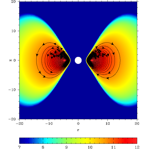
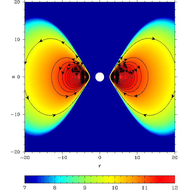
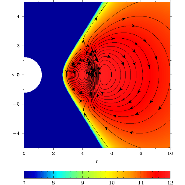
Figure 1: Initial conditions for the Low torus momentum (upper left panel), Quadrupole 1 (upper right panel), and Quadrupole 2 (lower panels) models. Initial distribution of the density logarithm and the initial magnetic field are shown by colours and lines, respectively.

2 Physical processes

2.1 Equation of state.

For the simulations we use the equation of state

$$P_{g}\equiv P(\rho,T)=P_{0}(\rho)+n_{b}kT+\frac{\sigma T^{4}}{3},$$ (1)

where $k$ is the Boltzmann constant, $\sigma$ is the radiation energy density constant, $n_{b}=\rho/m_{p}$ is concentration of baryons, $m_{p}$ is the mass of proton, $P$ is the pressure, $\rho$ is the density and $T$ is the temperature; $P_{0}(\rho)$ describes the ground level for the cold degenerate matter, the expression for $P_{0}(\rho)$ is an approximation of the table function from (Baym et al.1971b, Baym et al.1971a, Malone et al.1975).

The specific energy (per mass unit) was defined thermodynamically as

$$\epsilon=\epsilon_{0}(\rho)+\frac{3kT}{2m_{p}}+\frac{\sigma T^{4}}{\rho}.$$ (2)

The value of $\epsilon_{0}(\rho)$ was taken from (Bisnovatyi-Kogan2001). This equation of state allows us to deal with high-density matter. A more accurate EOS is significantly more expensive in calculations, while the disregarding of the $e^{+}e^{-}$-pair component in the plasma, for instance, can give a relative error in definition of the temperature less than $0.3$ at high temperatures (, Bisnovatyi-Kogan2001).

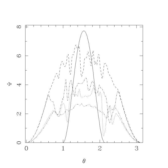
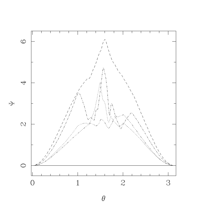
Figure 2: Time evolution of the magnetic flux $\Psi$ through the sphere of radius $r=4.7r_{g}$ (left panel) and through the horizon (right panel) in the case of the Low torus momentum. The fluxes at the moments $t=4.96\cdot 10^{-4}$ s., $t=0.0248$ s., $t=0.0495$ s., $t=0.0991$ s., $t=0.346$ s. are represented by solid, dashed, dot-dashed, dotted, and three-dots-dashed lines, respectively.

2.2 Neutrino cooling

On the grounds discussed in the introduction we ignore effects of neutrino heating in our simulations and take into account only the energy loss due to emission of neutrinos. Approximation formulas for the cooling rates due to $e^{+}e^{-}$ pair annihilation $Q_{p}$, neutrino photo-production $Q_{ph}$, and plasma mechanism $Q_{pl}$ are taken from (Schinder et al.1987), the cooling rate due to URCA processes $Q_{u}$ — from (Ivanova et al.1969), and the cooling rate due to synchrotron neutrino emission $Q_{s}$ — from (Bezchastnov et al.1997):

$$F_{\nu}(\rho,T)=Q_{p}+Q_{ph}+Q_{pl}+Q_{u}+Q_{s}.$$ (3)

The neutrino cooling is introduced by the source term in the energy-momentum equation

$$\partial_{\nu}(\sqrt{-g}T^{\nu}_{\mu})=\sqrt{-g}Su_{\mu},$$ (4)

where $u^{\nu}$ is the plasma four-velocity, $g$ is the determinant of the metric tensor, and $S$ is the cooling rate as measured in the fluid frame.

One of the aims of our research was the investigation of sensitivity of the torus accretion model to the neutrino cooling processes. We compare two cases: with no cooling at all and the optically thin case with neutrino cooling. The first instance is the most popular (, Gammie et al.2004, McKinney & Gammie 2004, McKinney & Narayan 2007, Hawley et al.2006, Beckwith et al.2008b) and less realistic. The second instance well suits for a light torus with the mass of a few per cent of the solar. It could be realized when two neutron stars or a neutron star and a black hole merge. The intermediate optical depth case is considered in Barkov (2008) and can be suitable for a collapsar model when the disk mass reaches several solar masses.

3 Simulation setup and the description of calculational models

3.1 General consideration

We make our calculation in the ideal relativistic MHD approximation using an upwind conservative scheme that is based on a linear Riemann solver and the constrained transport method to evolve the magnetic field. The details of this numerical method and its testing results are expounded in (Komissarov 1999); Komissarov (2004b); (Komissarov 2006).

The gravitational attraction of the black hole is introduced via Kerr metric in the Kerr-Schild coordinates, $\{\phi,r,\theta\}$. We set the black hole mass as $M_{BH}=10M_{\odot}$ which corresponds to $r_{g}=14.847$ km (we define $r_{g}\equiv GM_{BH}/c^{2}$). The two-dimensional axisymmetric computational domain is $(r_{in}<r<r_{out},0\leq\theta\leq\pi)$, where $r_{in}\equiv(1+\sqrt{1-a^{2}}/2)\;r_{g}$, $a\equiv cJ_{BH}/GM^{2}_{BH}$ is the dimensionless angular momentum of the black hole ($J_{BH}$ is the black hole angular momentum), and $r_{out}\equiv 200r_{g}\simeq 2969$ km. We adopt free-outflow as the outer and the inner boundary conditions. The inner boundary is located just inside the event horizon and adopts the free-flow boundary conditions. It is worthy of notice that the inner boundary is inside of the outer event horizon - this choice is possible since the horizon coordinate singularity is absent in the Kerr-Schild coordinates. The total mass within the domain is small (less than 25%) as compared with the mass of the black hole, which allows us to ignore its self-gravity. The grid is uniform over $\theta$, where it has 320 cells, and is almost uniform over $\log(r)$, where it has 459 cells, the linear size of each cell being the same in both directions.

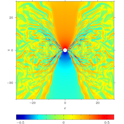
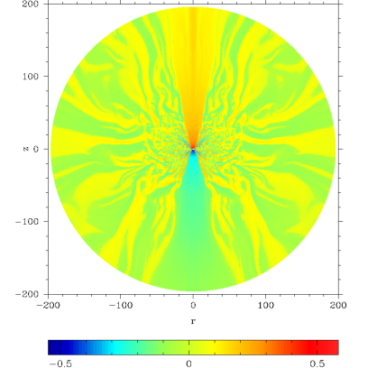
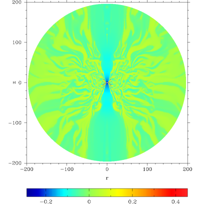
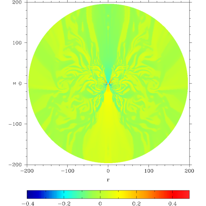
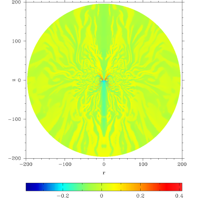
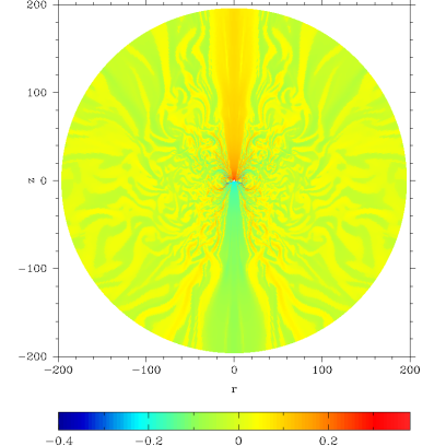
Figure 3: Distribution of $sign(B_{r})(|B_{r}|/10^{16}G)^{1/4}$ ($B_{r}$ is the radial component of the magnetic field). The upper panel represents the distribution at the moment $t=0.208$ s. for the central part of the Low torus momentum model (left picture), general view of the Low torus momentum model (central picture), and Quadrupole 1 model (right picture). The lower panel represents the distribution for the Quadrupole 2 model at the moments $t=0.1288$ s., $t=0.2278$ s., and $t=0.4259$ s.

As the initial distribution we consider an equilibrium torus (, Fishbone & Moncrief1976, Abramowicz et al.1978, Komissarov 2006) which is a ”torus” of plasma with the black hole in the centre. The value of the specific angular momentum $l_{0}$ determines the total effective potential which can be written as

$$W(r,\theta)=\frac{1}{2}\ln\left|\frac{L}{A}\right|,$$ (5)

where

$$L=g_{t\phi}g_{t\phi}-g_{tt}g_{\phi\phi}$$ (6)

and

$$A=g_{\phi\phi}+2l_{0}g_{t\phi}+l_{0}^{2}g_{tt}$$ (7)

Our numerical scheme cannot operate with vacuum. To avoid this difficulty, we have to introduce minimum possible values of the density and pressure that limit how small they can be. We also check the magnetic field and do not allow it to drop below the value defined by the equations $\rho_{min}\leq\dfrac{1}{6}\dfrac{B^{2}}{8\pi c^{2}}$ and $p_{min}\leq\dfrac{1}{100}\dfrac{B^{2}}{8\pi}$. For the magnetization typical of the task considered these inequalities are usually satisfied with a margin of three orders. The magnetic field strength is limited by the pair production by the neutrino-antineutrino annihilation and the Compton up scattering pair production (, Beskin et al.1992).

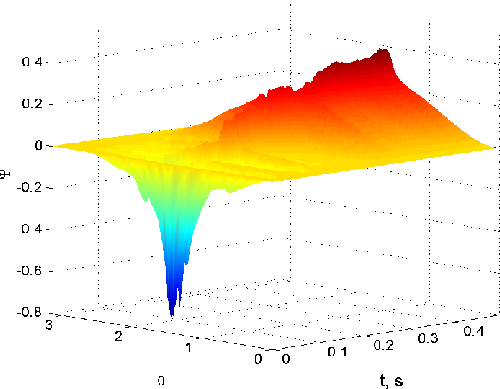
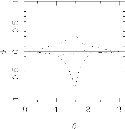
Figure 4: Time evolution of the magnetic flux $\Psi$ through the horizon for the Quadrupole 2 model. The left panel represents the time sections at $t=4.96\times 10^{-4}$ s., $t=0.0248$ s., $t=0.1238$ s., and $t=0.4452$ s. (solid, dashed, dotted, and three-dots-dished lines, respectively)

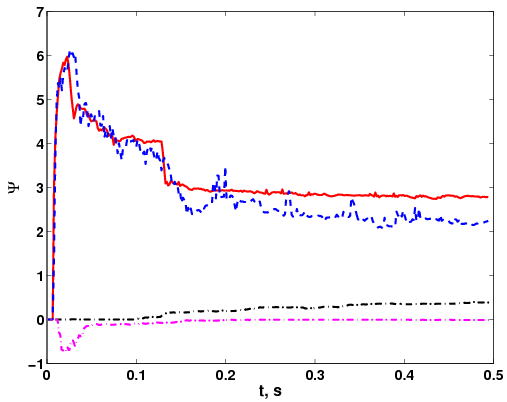
Figure 5: Time evolution of the maximum of the magnetic flux $\Psi$ through the horizon for the models: Low torus momentum (dashed line), Neutrino cooling (solid line), and Quadrupole 2 (dot-dashed-line)

3.2 Model choice

The parameter we are most interested in is the energy release effectiveness

$$\eta\equiv\frac{\int_{0}^{T}\dot{E}^{tot}dt}{\int_{0}^{T}\dot{M}_{BH}c^{2}dt}$$ (8)

where $\dot{E}^{tot}$ is the total energy flux at radius $180r_{g}$ and $\dot{M}_{BH}$ is the accretion rate on the horizon of the black hole. In order to test the effectiveness dependence on the accretion conditions, we introduce several models with various initial magnetic fields and other parameters.

The initial magnetic field structure in the disk is mainly determined by the dynamo effect. Dynamo in accretion disks was investigated by many authors (, Torkelsson & Branderburg1994; Arlt & Rüdiger, 1999; Bardou et al., 2001) in the context of $\alpha$-$\Omega$ model. Depending on the dynamo parameters, stationary dipole or quadrupole magnetic fields were obtained. Some models showed time oscillations. The calculations gave only a rough estimation of the magnetic field strength. To reproduce this simulations, we have chosen three different topologies of the initial magnetic field (similar to (Beckwith et al.2008a)).

Due to a strong dependence of the toroidal field component on the poloidal one, we initially introduce a purely poloidal magnetic field. This field can be described by a vector potential with a single nonzero component $A_{\phi}$. In our calculations we use

$$A_{\phi}\propto\left\{\begin{array}[]{cc}W(r,\theta)^{3}&\;\mbox{dipole field}\\ -W(r,\theta)^{3}\tanh\left(\frac{\theta-{\pi}/{2}}{w_{\theta}}\right)&\;\mbox{{\it Quadrupole 1} model}\\ -W(r,\theta)^{3}\tanh\left(\frac{r-r_{c}}{w_{r}r_{c}}\right)&\;\mbox{{\it Quadrupole 2} model}\end{array}\right.$$ (9)

where $w_{\theta}=0.05$ and $w_{r}=0.1$ are the parameters of the vector potential. We adopt a dipole initial magnetic field for Low torus momentum, High torus momentum, Neutrino cooling, Schwarzschild, and Low magnetized models. Model Quadrupole 1 possesses a quadrupole-like field generated by two dipoles: one is above and the second is below the equatorial plane. Quadrupole 2 model also has a quadrupole field, but the two dipoles are situated closer and farther from the black hole, which reproduces time oscillating magnetic field in the accretion disk. The topology of magnetic field is presented in Fig. 1. In all the cases the initial field is normalized so that the maximum of the magnetic to gas pressure ratio $\beta=P_{m}/P_{g}$ does not exceed $3\cdot 10^{-2}$, except for the Low magnetized model, where $\beta\leq 3\cdot 10^{-4}$. We have chosen the small value of $\beta$ in order to avoid strong influence of the magnetic pressure on the initial hydrodynamical equilibrium of the configuration.

The dimensionless angular momentum of the black hole is $a=0.9$ for all the models except for the Schwarzschild one, where $a=0$. The collapsing torus specific angular momentum and mass are equal to $l=2.8\cdot r_{g}c=1.247\cdot 10^{17}\;cm^{2}sec^{-1},M_{tor}=2.55M_{\odot}$ for Low torus momentum, Neutrino cooling, Quadrupole 1, Quadrupole 2 models and $l=4.0\cdot r_{g}c=1.782\cdot 10^{17}\;cm^{2}sec^{-1},M_{tor}=1.87M_{\odot}$ for High torus momentum, Schwarzschild, Low magnetized models. In all the models, except for Neutrino cooling, we neglect the neutrino cooling. The summary of the model parameters see in tab. 1.

Table 1: The list of model initial parameters.

model name	$l/(r_{g}c)$	$a$	$M_{tor}$	Neutrino cooling	Magnetic field type	$max(P_{m}/P_{g})$
Quadrupole 1	2.8	0.9	2.55	No	Up-down Quadrupole	$0.03$
Quadrupole 2	2.8	0.9	2.55	No	Farther-closer Quadrupole	$0.03$
Low torus momentum	2.8	0.9	2.55	No	Dipole	$0.03$
Neutrino cooling	2.8	0.9	2.55	Yes	Dipole	$0.03$
High torus momentum	4.0	0.9	1.87	No	Dipole	$0.03$
Schwarzschild	4.0	0.0	1.87	No	Dipole	$0.03$
Low magnetized	4.0	0.9	1.87	No	Dipole	$0.0003$

4 Results

All the models (except the Schwarzschild) after the first relaxation gave rise to the same standard configuration: a highly magnetized jet, a thick disk and the wind from it. Let us discuss the influence of various parameters of the system on the accretion rate and energy yield.

4.1 Magnetic field topology

Poloidal magnetic field plays a crucial role in the evolution and dynamics of the accretion disks. Magneto-rotational instability (MRI) defines the accretion rate and could be the source of the magnetic dynamo mechanism in the disk. Due to the 2D approach MRI cannot lead to the magnetic dynamo appearance in our calculations. It is easy to see that by the magnetic flux

$$\Psi(\theta)=\int^{\theta}_{0}\mn@boldsymbol{B_{p}}\!\cdot\!\mn@boldsymbol{dS}$$ (10)

decreases with time (Fig. 2, Low torus momentum model). First of all, we investigate the influence on our system of various magnetic field topologies.

A dipole-type Low torus momentum model exhibits a fast MRI growth in the disk. At first, we can see a powerful burst of energy extraction. It seems to be an effect of switching, after a while the flux becomes stationary. The accretion runs actively. Magnetosphere of the black hole is dipole-like (see Fig. 2). The magnetic flux through the horizon is of the same order as the initial one; the effectiveness of the total energy extraction $\eta$ is $\sim 7.4\times 10^{-4}$.

Quadrupole 1 model shows a slower growth of MRI. The magnetosphere of the black hole is monopole-like (see Fig. 3) and does not significantly change with time. The magnetic flux through the horizon is ten times reduced, compare to the initial one that results in a low energy extraction rate: $\eta$ is $1.1\times 10^{-5}$.

The magnetic field structure of the Quadrupole 2 model actually represents a configuration of two current frames on the different radii in the equatorial plane. In this case, the magnetosphere is dipole-like, but time variant. One can see on Fig. 3 that initially the magnetic lines near the black hole are predominantly oriented upward. As the inner currant frame is falling under the horizon, the magnetic field lines get the opposite direction. The mean magnetic flux is also ten times less than the initial one. The efficiency coefficient $\eta$ of the jet is $2.2\cdot 10^{-5}$.

In our calculations the accretion rate to the black hole is proportional to the maximum value of the magnetic flux module in the torus. On the other hand, the energy release in both the quadrupole cases drops down dramatically (up to 250 times, see tab. 2).

In the case of the Low magnetized model, the MRI grows very slowly. Accretion starts after a long ($0.6$ sec) phase of the field linear amplification in the torus up to $(P_{m}/P_{g})\sim 1$. When the accretion starts, the system takes on the standard appearance: a jet, an accretion disk and the wind from it. The energy release and the accretion rate are very low (see tab. 2). The efficiency $\eta$ of the wind is $2.0\times 10^{-5}$ and of the jet is $4.9\times 10^{-7}$.

4.2 Angular momenta of the torus and of the black hole

In the models Low torus momentum, Quadrupole 1, and Quadrupole 2 we put the torus angular momentum $l=2.8\cdot r_{g}c$ which is very close to the limit configuration, and even small perturbations lead to accretion. If the initial momentum is augmented to $l=4.0\cdot r_{g}c$ (High torus momentum model), it decreases the accretion rate thirty times but the energy release does not drop so strongly (see tab. 2), since a significant part of the field accretes on the black hole increasing the magnetic flux near it. As a result, the effectiveness of energy extraction in this case is high $\eta=3.0\times 10^{-3}$.

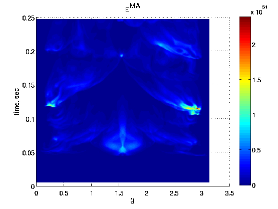
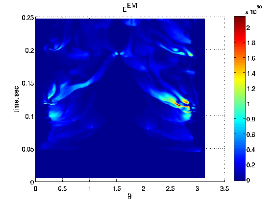
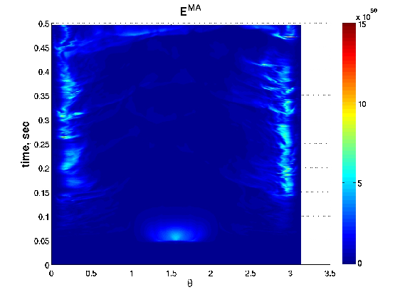
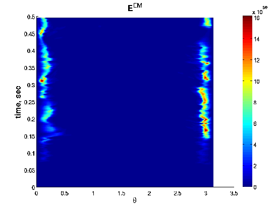
Figure 6: Dependence on $\theta$ and time of the matter ($\dot{E}^{MA}$, left panels) and electromagnetic ($\dot{E}^{EM}$, right panels) energy fluxes per unit angle at the radius $R=180r_{g}$ for the Schwarzschild (upper row) and High torus momentum (lower row) models.

Another important parameter is the angular momentum of the black hole $a$. Detailed investigations of its influence on the jet formation has been made in (Gammie et al.2004, McKinney & Gammie 2004); (McKinney2005); (Hawley et al.2006). The structure of the solution significantly changes if $a=0$ (Schwarzschild model, see tab. 2). The central highly magnetized jet does not appear at all, the energy is released through the subrelativistic magnetized wind. The total energy flux of the system jet-wind is almost the same for the Schwarzschild and the High torus momentum models, whereas the accretion rate in the former case is $27$ times higher.

Let us consider the time-space evolution of the energy flux at the distance $R=180\cdot r_{g}$. The total flux can be divided in two parts: electromagnetic ${\dot{E}}^{EM}$ and carried out by matter ${\dot{E}}^{MA}$. In the case of High torus momentum (Fig. 6, the lower row), it is easy to see that the flux is predominantly electromagnetic in the jets and matter-dominated in the wind. The maximal electromagnetic flux propagates near (not on) the axes. The maxima of the matter energy flux are strongly correlated with the electromagnetic maxima, as the main part of matter energy flux is driven by shock waves appearing at the boundary between the relativistic jets and the non-relativistic wind (the lines going up from the jet to the equatorial region). The jets very effectively heat the surrounding wind and can produce a hot corona around the disk.

In the case of Schwarzschild model, the situation is different (fig.6, the upper row): electromagnetic and matter energy fluxes have much wider angular distribution. A highly magnetized zone does not appear, and we can see a matter dominated magnetized outflow. Magnetic braking of the black hole produces the wind that carries out the magnetic field.

4.3 Neutrino cooling

In the initial torus configuration radiation and degenerated matter produce $80\%$ and $20\%$ of the total pressure, respectively. Therefore, neutrino cooling becomes very important.

Intensive neutrino cooling in the Neutrino cooling model (where the system is not opaque for neutrino propagation) leads to a significant disbalance in the initial distribution. The originally stable torus collapses to a new configuration with negligible thermal pressure. One can see the influence of neutrino cooling on the structure of the torus in Fig. 7. The torus without cooling keeps the initial size and shape. The cooling leads to a collapse of the initial configuration. The maximum density increases up to ten times and reaches the value $10^{13}$ g/cm³.

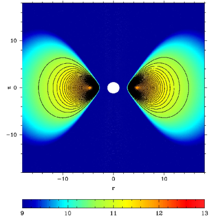
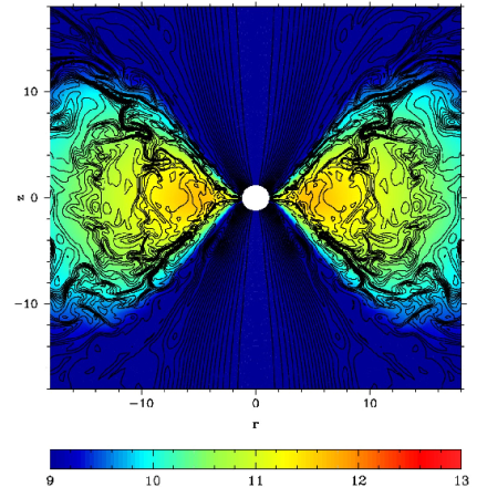
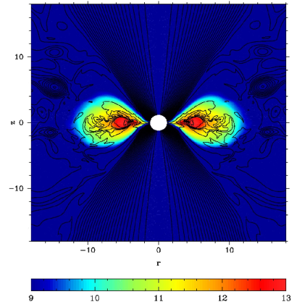
Figure 7: Distribution of $\log_{10}(\rho)$ and magnetic lines. Left panel represents the initial distribution. Central and right panels represent the distributions after 0.2075 s. of evolution for the Low torus momentum and Neutrino cooling models are shown on the central and right panel, respectively.

The structure of the accretion flow does not change significantly: the Neutrino cooling model flow is similar to High torus momentum (Fig. 7) and thinner than in Low torus momentum model. The Low torus momentum model has a much smaller and less stable highly magnetized jet region than in the Neutrino cooling case (Fig. 8). Despite the fact that the Neutrino cooling accretion rate is two times lower than the Low torus momentum one (tab. 2), the energy release and the magnetic flux through the horizon are even slightly higher in the Neutrino cooling model (Fig. 5). So Neutrino cooling and High torus momentum models have the same effectiveness coefficient $\eta\sim 0.003$ that is $2-4$ times greater than for the Low torus momentum model.

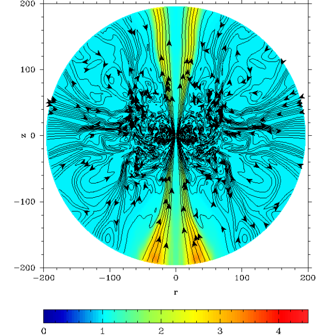
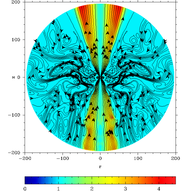
Figure 8: Lorenz factor distribution for $t=0.2075$ s. Left panel represents the Low torus momentum model with no cooling, the right one — Neutrino cooling model.

At the inception of the calculations the central region of the torus rapidly cools down and falls to the potential hollow, while the outer parts do not cool at first. Intensive neutrino cooling leads to a disbalance in the accretion torus. Due to asymmetry of the potential well, uncompensated gravitational forces give rise to oscillations (Fig. 9, similar results were obtained by (Zanotti et al.2005); (Montero et al.2007)). So the cooling produces intensive radiative shock waves, that (as well as the poloidal magnetic field) strongly increases the effective viscosity. When we neglect the cooling, the oscillations do not appear, the mean radius increases due to the strong wind outflow. In the optically thin case, the oscillations appear with the amplitude ${\Delta r^{m}/r^{m}}=0.05$, where $r^{m}=\int_{M}|r|dm/\int_{M}dm$ is the mean mass radius, and quickly degrade due to the high viscosity. We can estimate the relaxation time as $t_{relax}=t_{osc}\times Q$, where $Q=|(\Delta r_{i}^{m}+\Delta r^{m}_{i+1})/2(\Delta r^{m}_{i}-\Delta r^{m}_{i+1})|\simeq 3.8$ and $\Delta r^{m}_{i}$ is the maximal deviation from the equilibrium of the $i$-th oscillation. In our case $t_{relax}\approx 0.027$ sec. The same oscillations were obtained in the case of intermediate neutrino optical depth (Barkov, 2008).

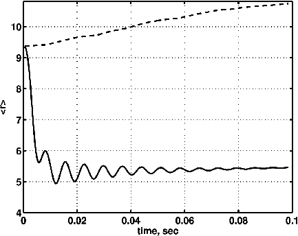
Figure 9: Mean radius $r^{m}$ evolution for Low torus momentum (dashed line) and Neutrino cooling (solid line) models.

Table 2: Main results.

model	$l$	$a$	$\dot{M}_{BH}$	$\dot{M}_{w}$	${\dot{E}}^{EM}_{51}$	${\dot{E}}^{MA}_{51}$	${\dot{E}}^{tot}_{51}$	$\eta$
Low torus momentum	2.8	0.9	1.3937	0.0189	0.777	1.076	1.8530	$7.4\times 10^{-4}$
Neutrino cooling	2.8	0.9	0.8588	0.0134	1.5024	1.4014	2.9039	$1.9\times 10^{-3}$
Quadrupole 1	2.8	0.9	0.3976	0.00023	0.0022	0.0058	0.0080	$1.1\times 10^{-5}$
Quadrupole 2	2.8	0.9	0.2126	0.00034	0.0019	0.0065	0.0083	$2.2\times 10^{-5}$
High torus momentum	4.0	0.9	0.053	0.0026	0.1283	0.1541	0.2824	$3.0\times 10^{-3}$
Schwarzschild model	4.0	0.0	1.411	0.0086	0.0216	0.2320	0.2536	$1.0\times 10^{-4}$
Low magnetized	4.0	0.9	0.0023	$5.5\times 10^{-6}$	$2.0\times 10^{-6}$	$8.16\times 10^{-5}$	$8.36\times 10^{-5}$	$2.0/0.049\times 10^{-5}$

Here $l$ is the dimensionless angular momentum of the accreting matter; ${\dot{M}_{BH}}$ — accretion rate $M_{\odot}\mbox{s}^{-1}$; $\dot{M}_{w}$ – wind mass loss rate $M_{\odot}\mbox{ s}^{-1}$ at radius $180r_{g}$; ${\dot{E}}^{EM}_{51}$, ${\dot{E}}^{MA}_{51}$, ${\dot{E}}^{tot}_{51}$ are electromagnetic energy, matter energy, and the total energy fluxes at radius $180r_{g}$, $10^{51}\mbox{ erg }\mbox{s}^{-1}$ ; $\eta$ — accretion effectiveness (8) (for the Low magnetized model we present separately the effectiveness of the electromagnetic energy extraction). Notice that in the case of the Low magnetized model the accretion starts only after $0.75$ s., while the calculation ends at $0.99$ s.

5 Discussion

Topology and strength of the magnetic field play a crucial role in the process of accretion on a black hole. In our simulations the energy release effectiveness varies over two orders of magnitude when we change the magnetic field topology from the dipole (Neutrino cooling, High torus momentum models) to the quadrupole one(Quadrupole 1, Quadrupole 2 models). Due to the 2D approach we cannot consider the dynamo effect. However, we can see temporal increases of the magnetic field intensity owing to the MRI-driven turbulence growth and magnetic line twist.

The Blandford-Znajek mechanism plays a leading role in accreting black hole energy release. For a force-free monopole magnetosphere the Blandford-Znajek power is given by

$$\dot{E}_{BZ}=\frac{1}{6c}\left(\frac{\Omega\Psi}{4\pi}\right)^{2},$$ (11)

We assume $\Omega=\Omega_{h}/2$, were $\Omega_{h}=a/2(1+\sqrt{1-a^{2}})$ is the angular velocity of the black hole and $\Psi$ is the magnetic flux (10) threading the black hole.

Our estimations of the energy release effectiveness differ by a factor of $3$ from (McKinney2005) and by a factor of up to $25$ from Barkov & Komissarov (2008b); (Komissarov & Barkov 2009). We explain it by distinctions between the initial magnetic fields: in (Komissarov & Barkov 2009), for instance, the magnetic field flux was $4.8$ times higher.

Neutrino cooling processes significantly suppress the wind from the accretion disk, but do not diminish appreciably the energy release; moreover, sometimes they can stabilize the outflow. The neutrino driven oscillations (Fig. 9) look like an artificial effect of turning on the initial conditions: more realistic conditions like (MacFadyen et al.1999); Barkov & Komissarov (2008a) do not lead to significant radial oscillations. But even if the effect is real, the oscillations (, MacFadyen et al.1999) can scarcely be observed by gravitational wave detectors.

Highly magnetized jets appear in all the models considered, where the black hole possesses angular momentum. The obtained parameters of the plasma acceleration in the jets (Fig. 8) are in good agreement with Komissarov et al. (2007a); Barkov & Komissarov (2008b); Komissarov et al. (2009).

The boundary between the jet and the wind is unstable (the perturbation growth is most pronounced in Fig. 8, Neutrino cooling case, in the south hemisphere in the radius interval $100-150r_{g}$. (McKinney2006) reported about a similar effect). The jet speed is much higher than the sound speed in the wind, and the boundary perturbations generate strong shock waves propagating to the wind region (Fig.6). The shocks effectively heat the wind and can produce a hot corona around the accretion disks like in the SS433 system (, Cherepashchuk et al.2006).

If we adopt the effectiveness coefficient $\eta\sim 0.003$ of the models Neutrino cooling and High torus momentum, it allows us to estimate the total energy release of the torus accretion as $E_{tot}\approx\eta M_{torus}c^{2}\approx 1.3\cdot 10^{52}$ erg. This value of $\eta$ however, need not to be universal: as we saw, other magnetic field topologies can have a significantly different efficiency.

The scenario considered in this article is a possible alternative to the magnetar-driven hypernova scheme (Komissarov & Barkov, 2007b). Both the scenarios predict the appearance of collimated jets energetic enough to explain GRB as well as hypernovae phenomena. Accurate calculations are needed to find characteristic features and distinguish these two schemes. By now we can say that the chemical composition of matter in the jets should be different. In the collapsar scenario we expect a highly Poynting-dominated jet ($\epsilon_{field}/\epsilon_{matt}\sim 1000$, where $\epsilon_{field}$ and $\epsilon_{matt}$ are the field and the matter energy flux densities, respectively), mainly made up of $e^{+}e^{-}$-pairs, while in the magnetar-driven scenario the jet is baryon-dominated and intermediately magnetized ($\epsilon_{field}/\epsilon_{matt}\sim 1-100$).

The effect of the magnetic field sign change found in the jet of the Quadrupole 2 model, may be the key to understanding of the ”surprising evolution of the parsec-scale Faraday rotation gradients in the jet of the BL Lac object B1802+784” (, Mahmud et al. 2009). Complicated topology of the magnetic field in the accretion disk can lead to variations of the magnetic field direction in the jet. In this case, the jet constitutes a chain of regions with various magnetic field orientations.

6 Conclusion

The accretion rate and energy release are governed by four main parameters: magnetic field structure, angular momentum of the black hole, specific angular momentum of the accreting matter, accretion disk mass or accreting part of the star envelop. To have a long-time accretion, angular momentum of the accreting matter should be high enough to form an accretion disk around the black hole. As it has been demonstrated by the Schwarzschild model, if the black hole has deficient angular momentum, the powerful magnetized jet does not appear at all, which totally changes the picture of the accretion. Moreover, a comparison of the Low and High torus momentum models shows us that a respectively small variation of the angular momentum of the accreting matter leads to a change of the accretion efficiency. Neutrino losses do not prevent energy release and can even stabilize the magnetized jet outflow.

The least understood and a very important factor defining the accretion efficiency is the disk magnetic field structure. As we could see from the calculations, a mere replacing of the dipole field by the quadrupole one decreases the energy release by two orders of magnitude. The magnetic flux $\Psi$ governs the energy extraction from ergosphere (11), while the black hole magnetosphere is formed and supported by the disk. In our calculations we preset the initial magnetic field in the torus. It is clear, however, that self-consistent numerical calculations of the magnetic dynamo in the disk are necessary in order to elucidate the problem.

Nevertheless, our calculations show that a very intensive electromagnetic and matter energy flux can be evolved during massive torus accretion on a rotating black hole with mass $\sim 10M_{\odot}$. The total energy budget is quite sufficient to explain hypernova explosions like GRB 980425 or GRB 030329. The magnetized matter accretion on a rotating black hole is a very promising model of the central engine of these phenomena.

In addition, we have found that the instability of the boundary between the jet and the wind generates shock waves propagating to the wind region and heating it. This effect can give rise to a hot corona around the binary system similar to SS433.

References

- (1) Abramowicz M., Jaroszynski M., Sikora M., 1978, A&A, 63, 221
- Aloy et al. (2000) Aloy M.A., Müller E., Abner J.M., Marti J.M., MacFadyen A.I., 2000, ApJ, 531, L119
- Ardeljan et al. (2005) Ardeljan N.V., Bisnovatyi-Kogan G.S., Moiseenko S.G., 2005, MNRAS, 359, 333
- Arlt & Rüdiger (1999) Arlt R., Rüdiger G., 1999, A&A, 349, 334
- Bahcall (1964) Bahcall J.N., 1964, Phys. Rev. B, 136, 1164
- Bardou et al. (2001) Bardou A., von Rekowski B., Dobler W. , Brandenburg A., Shukurov A., 2001, A&A, 370, 635
- Balbus & Hawley (1991) Balbus S.A., Hawley J.F., 1991, ApJ, 376, 214
- Barkov (2008) Barkov M.V., 2008, in COOL DISCS, HOT FLOWS, AIP Conference Proceedings, v. 1054, p. 79
- Barkov & Komissarov (2008a) Barkov M.V., Komissarov S.S., 2008a, MNRAS, 385, L28
- Barkov & Komissarov (2008b) Barkov M.V., Komissarov S.S., 2008b, IJMP D, 17, 1669
- Barkov & Komissarov (2009) Barkov M.V., Komissarov S.S., 2009, in preparation
- Baushev & Chardonnet (2009) Baushev A.N., Chardonnet P., 2009, in press (arXiv:0905.4071)
- (13) Baym G., Bethe H., Pethick Ch., 1971, NP, A175, 255
- (14) Baym G., Pethick Ch., Sutherland P., 1971, ApJ, 170, 306
- (15) Beckwith K., Hawley J., Krolik J., 2008, ApJ, 678, 1180
- (16) Beckwith K., Hawley J., Krolik J., 2008, MNRAS, 390, 21
- (17) Beskin V.S., Istomin Ya.N., Par’ev V.I., 1992, SvA, 36, 642
- (18) Bezchastnov V.G., Haensel P., Kaminker A.D., Yakovlev D.G., 1997, A&A, 328, 409
- (19) Birkl R., Aloy M.A., Janka H.Th., Müller E., 2007, A&A, 463, 51
- (20) Bisnovatyi-Kogan G.S., 2001, Springer, Stellar physics. Vol.1
- (21) Blandford R.D. and Znajek R.L.,1977,MNRAS,179,433
- (22) Blandford R.D., Payne D.G.,1982,MNRAS,199,883
- (23) Blinnikov S.I., Postnov K.A., Kosenko D.I., Bartunov O.S., 2005, Astron. Lett., 31, 6, 365
- (24) Bloom J.S., Kulkarni S.R., Djorgovski S.G., 2002, AJ, 123, 1111
- (25) Chandrasekhar S., 1960, Proc. Nat. Acad. Sci. USA, 46, 253
- (26) Cherepashchuk A.M., Sunyaev R.A., Seifina E.V., Antokhina E.A., Kosenko D.I., Molkov S. V., Shakura N. I., Postnov K. A. et al., 2006, astro-ph/0610235
- (27) De Villiers J.P., Hawley J.F., Krolik J.H., 2003, ApJ, 599, 1238
- (28) Fishbone L.G., Moncrief V., 1976, ApJ, 207, 962
- (29) Fishman G.J., Meegan C.A., 1995, Ann. Rev. Astron. Ap., 333, 415
- (30) Fruchter A.S., Levan A.J., Strogler L., Vreeswijk P.M., Thorsett S.E., Bersier D., Burud I., Castro Cerón J.M. et al., 2006, Nature, 441, 7092, 463
- (31) Galama T.J., Vreeswijk P.M., van Paradijs J., Kouveliotou C., Augusteijn T., Böhnhardt H., Brewer J.P., Doublier V. et al., 1998, Nature, 395, 6703, 670
- (32) Greiner J., Peimbert M., Estaban C., Kaufer A., Jaunsen A., Smoke J., Klose S., Reimer O., 2003, GCN 2020
- (33) Gammie C.F., McKinney J.C., 2004, ApJ, 602, 312
- (34) Hawley J.F., Krolik J.H., 2006, ApJ, 641, 103
- (35) Hjorth J., Sollerman J., Møller P., Fynbo J.P.U., Woosley S.E., Kouveliotou C., Tanvir N.R., Greiner J. et al., 2003, Nature, 423, 6942, 847
- (36) Ivanova L.N., Imshennik V.S., Nadezhin D.K., 1969, NI, 13, 3
- (37) Klebesadel R.W., Strong I.B., Olson R.A., 1973, ApJL, 182, L85
- (38) Kouveliotou C., Meegan C.A., Fishman G.J., Bhat N.P., Briggs M.S., Koshut T.M., Paciesas W.S., Pendleton G.N. , 1993, ApJL, 413, L101
- (39) Komissarov S.S., 1999, MNRAS, 303, 343
- Komissarov (2004b) Komissarov S.S., 2004b, MNRAS, 350, 1431
- (41) Komissarov S.S., 2006, MNRAS, 368, 993
- Komissarov & Barkov (2007b) Komissarov S.S., Barkov M.V., 2007, MNRAS, 382, 1029
- Komissarov et al. (2007a) Komissarov S.S., Barkov M.V., Vlahakis N., Königl A., 2007b, MNRAS, 380, 51
- Komissarov et al. (2009) Komissarov S.S., Vlahakis N., Königl A., Barkov M.V., 2009, MNRAS, 394, 1182
- (45) Komissarov S.S., Barkov M.V., 2009, arXiv:0902.2881, accepted by MNRAS
- (46) MacFadyen A.I., Woosley S.E., 1999, ApJ, 524, 262
- (47) Malone R.C., Johnson M.B., Bethe H.A., 1975, ApJ, 199, 741
- (48) Matheson T., Garnavich P.M., Stanek K.Z., Bersier D., Holland S.T., Krisciunas K., Caldwell N., Berlind P. et al., 2003, ApJ, 599, 394
- (49) Mazets E.P. and Golenetskii S.V., 1981, Ap&SS, 75, 1, 47
- (50) MacFadyen A.I., Woosley S.E, 1999, ApJ,524, 262
- (51) Mahmud M., Gabuzda D.C., Bezrukovs V., 2009, arXiv:0905.2368
- (52) McKinney J.C., Gammie C.F., 2004, ApJ, 611, 977
- (53) McKinney J.C., ApJL, 630, L5
- (54) McKinney J.C., MNRAS, 368, 1561
- (55) McKinney J.C., Narayan R., 2007, MNRAS, 375, 513
- (56) McKinney J.C., Blandford R.D., 2009, MNRAS, 394, L126
- (57) Montero P.J., Zanotti O., Font J.A., Rezzolla L., 2007, MNRAS, 378, 1101
- (58) Nagataki S., Takahashi R., Mizuta A., Takiwaki T., 2007, ApJ, 659, 512
- (59) Nagataki S., 2009, arXiv:0902.1908
- (60) Pian E., Amati L., Antonelli L.A., Butler R.C., Costa E., Cusumano G., Danziger J., Feroci M. et al., 2000, ApJ, 536, 778
- (61) Popham R., Woosley S.E., Fryer C., 1999, ApJ, 518, 356
- Proga et al. (2003) Proga D., MacFadyen A.I., Armitage P.J., Begelman M.C., 2003, ApJ, 629, 397
- (63) Shakura N.I., Sunyaev R.A., 1973, A&A, 24, 337
- (64) Schinder P. J., Schramm D. N., Wiita P. J., Margolis S. H., Tubbs D. L., 1987, ApJ, 313, 531
- (65) Shibata M., Sekiguchi Yu, Takahashi R., 2007, PThPh, 118, 2, 257
- (66) Soffitta P., Feroci M., Piro L., in ’t Zand J., Heise J., di Ciolo L., Muller J.M., Palazzi E. et al., 1998, IAU Circular No. 6884
- (67) Sokolov V.V., Fatkhullin T.A., Komarova V.N., Kurt V.G., Lebedev V.S., Castro-Tirado A.J., Guziy S., Gorosabel J. et al., 2003, BSAO, 56, 5
- (68) Thompson T.A., Burrows A., Meyer B.S., 2001, ApJ, 562, 887
- (69) Torkelsson U., Brandenburg A., 1994, A&A, 283, 677
- (70) Tubbs D.L., Schramm D.N., 1975, ApJ, 201, 467
- (71) Uzdensky D.A., MacFadyen A.I., 2006,ApJ,647,1192
- (72) Velikhov E.P., 1959, Sov. Phys. JETP, 36, 995
- (73) Woosley S.E., 1993,ApJ,405,273
- (74) Zalamea I., Beloborodov A.M., 2008, arXiv:0812.4041
- (75) Zanotti O., Font J.A., Rezzolla L., Montero P.J., 2005, MNRAS, 356, 1371