Fictitious-time wave-packet dynamics in atomic systems

Abstract

Gaussian wave packets (GWPs) are well suited as basis functions to describe the time evolution of arbitrary wave functions in systems with nonsingular smooth potentials. They are less so in atomic systems on account of the singular behavior of the Coulomb potential. We present a time-dependent variational method that makes the use of GWPs possible in the description of propagation of quantum states also in these systems. We do so by a regularization of the Coulomb potential, and by introduction of a fictitious time coordinate in which the evolution of an initial state can be calculated exactly and analytically for a pure Coulomb potential. Therefore in perturbed atomic systems variational approximations only arise from those parts of the potentials which deviate from the Coulomb potential. The method is applied to the hydrogen atom in external magnetic and electric fields. It can be adapted to systems with definite symmetries, and thus allows for a wide range of applications.

1 Introduction

Wave packets in atomic systems can be excited experimentally, e.g., with microwaves [1, 2, 3] or short laser pulses [4, 5]. Theoretically, the time evolution of wave packets can be calculated accurately by numerically solving the time-dependent Schrödinger equation [6], or by using approximation methods, such as semiclassical [7] or time-dependent variational [8] methods. The topic of wave packet dynamics in systems with Coulomb interactions covers a large body of problems ranging from atomic physics to physics of solid state, where Coulomb interaction plays an important, often crucial, role. In many-body physics, in particular, in the physics of solid state, theoretical methods well suited for studying the effects stemming from Coulomb interactions are still lacking. The majority of the available methods, e.g., the method of pseudopotentials in atomic physics and the Fermi and the Luttinger liquid theories for solid conductors, are basically indirect and substantiated neither from the theoretical nor from the experimental side. For this reason they still remain, to a certain extent, disputable. The time-dependent variational principle (TDVP) applied to Gaussian wave packets (GWPs) lead to exact results for the harmonic oscillator potential. GWPs have turned out to be also well suited for describing the time evolution of arbitrary wave functions in smooth and nearly harmonic potentials [9, 10] but they are bound to fail for atomic systems because of the singularity of the Coulomb potential. It is the objective of this Letter to make the GWP method applicable to the description of the time evolution of arbitrary quantum states also in these systems.

For the one-dimensional (1D) Coulomb potential, attempts already have been made [11, 12, 13] to use GWPs as trial wave functions, based on a local harmonic approximation. For the full 3D Coulomb potential, which we will consider, a way to remove the singularity is, as is well known, the transformation to 4D Kustaanheimo-Stiefel (KS) coordinates [14, 15], which converts the Coulomb potential into a sum of two 2D harmonic oscillator potentials, adapted to the use of GWPs, but also introduces an additional constraint on the wave functions. The regularization implies a fictitious time coordinate. Various approaches have been made to construct coherent states for the hydrogen atom [16, 17, 18, 19, 20] in the fictitious time in analogy with the coherent states of the harmonic oscillator. These approaches construct the coherent states as the eigenstates of the lowering operators associated with the harmonic potential.

We will present a variant of the GWP method in coordinate space, which describes wave packet propagation in the Coulomb problem exactly. Therefore it is only deviations from the Coulomb potential which require a variational treatment. As prime examples we will apply the method to wave packet propagation in the hydrogen atom in a magnetic field, and in crossed electric and magnetic fields. Both systems have attracted considerable attention over the past decades because classically they exhibit a transition from regular to chaotic motion and thus can be used in the search for quantum signatures of chaos [21, 22]. If the method can be further extended to larger systems with more degrees of freedom it will allow for a wide range of future applications in different branches of physics.

2 Restricted Gaussian wave packets

The Hamiltonian for an electron under the combined action of the Coulomb potential and external perpendicularly crossed electric and magnetic fields has the form (in atomic units, with $F_{0}=5.14\times 10^{9}$ V/cm, $B_{0}=2.35\times 10^{5}$ T)

$$H_{3}=\frac{1}{2}{\bf p}^{2}-\frac{1}{r}+\frac{1}{2}Bl_{z}+\frac{1}{8}B^{2}(x^{2}+y^{2})+Fx\;.$$ (1)

Here we have assumed that the electric field is oriented along the $x$ axis, and the magnetic field along the $z$ axis. We regularize the singularity of the Coulomb potential by switching to KS coordinates ${\bf u}$ with $x=u_{1}u_{3}-u_{2}u_{4}$, $y=u_{1}u_{4}+u_{2}u_{3}$, and $z=\frac{1}{2}(u_{1}^{2}+u_{2}^{2}-u_{3}^{2}-u_{4}^{2})$. Introducing scaled coordinates and momenta ${\bf u}\to n_{\rm eff}^{1/2}{\bf u}$, ${\bf p}_{u}\to n_{\rm eff}^{-1/2}{\bf p}_{u}$ one obtains

$$H\psi=\left[\frac{1}{2}{\bf p}_{u}^{2}+V({\bf p}_{u},{\bf u})\right]\psi=2n_{\rm eff}\,\psi\;,$$ (2)

where the scaled potential $V$ depends on the parameters

$$\alpha\equiv-n_{\rm eff}^{2}E\;,\quad\beta\equiv n_{\rm eff}^{2}B\;,\quad\zeta\equiv n_{\rm eff}^{3}F\;,$$ (3)

which can be chosen constant. Eq. (2) is an eigenvalue problem for the effective quantum number $n_{\rm eff}$, and for any quantized $n_{\rm eff}$ the energy $E$ and field strengths $B$ and $F$ of the physical state are obtained from Eq. (3). In KS coordinates physical wave functions must fulfill the constraint

$$(u_{2}p_{1}-u_{1}p_{2}-u_{4}p_{3}+u_{3}p_{4})\,\psi=0\;.$$ (4)

For $\alpha=1/2$ and vanishing external fields ($\beta=0$, $\zeta=0$) Eq. (2) describes the 4D harmonic oscillator with $V=\frac{1}{2}{\bf u}^{2}$, and $n_{\rm eff}=n$ becomes the principal quantum number of the field-free hydrogen atom.

Eq. (2) can be extended to the time-dependent Schrödinger equation in a fictitious time $\tau$ by the replacement $2n_{\rm eff}\to i\frac{\partial}{\partial\tau}$, viz.

$$i\frac{\partial}{\partial\tau}\psi=\left(\frac{1}{2}{\bf p}_{u}^{2}+V\right)\psi=H\psi\;.$$ (5)

When the TDVP is used to solve Eq. (5) the wave function $\psi$ depends on a set of appropriately chosen parameters whose time-dependences are obtained by solving ordinary differential equations. As the regularized Hamiltonian without external fields (2) becomes that of a harmonic oscillator basis trial wave functions in the form of GWPs

$$g(A,{\bf q},{\bm{\pi}},\gamma)=e^{i[({\bf u}-{\bf q})A({\bf u}-{\bf q})+{\bm{\pi}}\cdot({\bf u}-{\bf q})+\gamma]}$$ (6)

with time-dependent parameters are a natural choice. In (6) $A$ designates a complex symmetric $4\times 4$ width matrix with positive definite imaginary part, ${\bm{\pi}}$ and ${\bf q}$ are the expectation values of the momentum and position operator, and the phase and normalization are given by the complex scalar $\gamma$. In KS coordinates physical wave functions must fulfill the constraint (4). Inserting the ansatz (6) into (4) leads to restrictions for the admissible variational parameters, viz. ${\bf q}=0$, $\bm{\pi}=0$, and the special form of the width matrix

$$A=\left(\begin{array}[]{crcr}a_{\mu}&0&a_{x}&a_{y}\\ 0&a_{\mu}&a_{y}&-a_{x}\\ a_{x}&a_{y}&a_{\nu}&0\\ a_{y}&-a_{x}&0&a_{\nu}\end{array}\right)\;,$$ (7)

which depends only on four parameters $(a_{\mu},a_{\nu},a_{x},a_{y})$ [23, 24]. The “restricted Gaussian wave packets” obeying Eq. (4) are located around the origin with zero mean velocity and thus at first glance might not appear appropriate for dynamical calculations. However, they are the key for both the exact analytical derivation of the fictitious time wave packet dynamics in the field-free hydrogen atom and the time-dependent variational approach to the perturbed atom.

The restricted GWPs are not a complete basis set for the four-dimensional harmonic oscillator but they are in the 3D space, i.e., any physically allowed state can be expanded in that basis. This can be verified by transforming the restricted GWP in KS coordinates back into 3D Cartesian coordinates,

$$g({\bf y}) =e^{i({\bf u}A{\bf u}+\gamma)}$$ (8a)

$$=e^{i[(a_{\mu}+a_{\nu})r+(a_{\mu}-a_{\nu})z+2a_{x}x+2a_{y}y+\gamma]}$$ (8b)

$$=e^{i(p_{r}r+{\bf p}\cdot{\bf x}+\gamma)}\;.$$ (8c)

In (8c) the set of parameters $(a_{\mu},a_{\nu},a_{x},a_{y},\gamma)$ is replaced with an equivalent set ${\bf y}=(p_{r},{\bf p},\gamma)$ with

$$p_{r}=a_{\mu}+a_{\nu}\,,\;{\bf p}=(p_{x},p_{y},p_{z})=(2a_{x},2a_{y},a_{\mu}-a_{\nu})\;.$$ (9)

For $p_{r}=0$ and real valued parameters $p_{x},p_{y},p_{z}$ the restricted GWP in Cartesian coordinates (8c) reduces to a plane wave. Since plane waves form a complete basis we have the result that the restricted GWPs (8) are also complete, or even over-complete.

3 Time-dependent variational principle

The propagation of the wave packets is investigated by applying the TDVP. Briefly, the TDVP of McLachlan [25], or equivalently the minimum error method [26], requires to minimize the deviation between the right-hand and the left-hand side of the time-dependent Schrödinger equation with the trial function inserted. The quantity

$$I=||i\phi(\tau)-H\psi(\tau)||^{2}\overset{!}{=}\min$$ (10)

is to be varied with respect to $\phi$ only, and then $\dot{\psi}\equiv\phi$ is chosen, i.e., for any time $\tau$ the fixed wave function $\psi(\tau)$ is supposed to be given and its admissible time derivative $\dot{\psi}(\tau)$ is determined by the requirement to minimize $I$. As trial functions we consider superpositions of $N$ restricted GWPs (8a), i.e.,

$$\psi(\tau)=\psi({\bf z}(\tau))=\sum_{k=1}^{N}g({\bf y}^{k})\equiv\sum_{k=1}^{N}g^{k}\;,$$ (11)

which are parameterized by a set of $5N$ time-dependent complex parameters ${\bf z}=({\bf y}^{k},k=1,\dots,N)$ [instead of $15N$ complex parameters when using the most general superposition of Gaussian wave packets (6) in 4D coordinate space]. The equations of motion for the variational parameters ${\bf z}(\tau)$ are obtained as

$$\dot{A}^{k} =-2(A^{k})^{2}-\frac{1}{2}V_{2}^{k}\;,$$ (12a)

$$\dot{\gamma}^{k} =i\,{\rm tr}\,A^{k}-v_{0}^{k}\;,$$ (12b)

where we have introduced the time-dependent scalars $v_{0}^{k}$ and matrices $V_{2}^{k}$, which induce couplings between the restricted GWPs. Since the special structure of the matrices $A^{k}$ in Eq. (7) is maintained in the squared matrices $(A^{k})^{2}$, that structure carries over to the $4\times 4$ complex symmetric matrices $V_{2}^{k}$. Therefore, they have only four independent coefficients $(V_{\mu}^{k},V_{\nu}^{k},V_{x}^{k},V_{y}^{k})$, in the notation of Eq. (7). The parameters $v_{0}^{k}$ and $V_{2}^{k}$ are calculated at each time step by solving a $5N$ dimensional set of linear equations. All integrals required for the setup of that linear system have the form $\langle g^{l}|f({\bf u},{\bf p}_{u})|g^{k}\rangle$, with $f({\bf u},{\bf p}_{u})$ a polynomial in the KS coordinates and momenta, and can be calculated analytically [24].

For the field-free hydrogen atom one finds $v_{0}^{k}=0$ and $V_{2}^{k}={\bm{1}}$, i.e., the equations of motion (12) simplify to the uncoupled equations $\dot{A}=-2A^{2}-\frac{1}{2}{\bm{1}}$, $\dot{\gamma}=i\,{\rm tr}\,A$ for the parameters of each each basis state. These equations can be solved analytically [23] and yield for the time evolution of the restricted GWP the explicit form

$$g(\tau)=\frac{1}{\mathcal{N}(\tau)}\exp\left\{i\,\frac{\mathcal{Z}(\tau)}{\mathcal{N}(\tau)}\right\}\;,$$ (13)

with

$${\mathcal{Z}(\tau)} ={\bf p}^{0}\cdot{\bf x}+p_{r}^{0}r\cos 2\tau+\frac{r}{2}[(p_{r}^{0})^{2}-({\bf p}^{0})^{2}-1]\sin 2\tau\;,$$ (14a)

$${\mathcal{N}(\tau)} =1+[(p_{r}^{0})^{2}-({\bf p}^{0})^{2}](1-\cos 2\tau)+p_{r}^{0}\sin 2\tau\;,$$ (14b)

and where $p_{r}^{0}$ and ${\bf p}^{0}$ are the parameters (9) of the initial GWP at time $\tau=0$. This is an important result for the field-free hydrogen atom: The time evolution of a restricted GWP (8c) can be calculated analytically, and takes the compact form (13), which is a periodic function of the fictitious time $\tau$ with period $\pi$. In the physical time wave packets disperse in the hydrogen atom. By contrast, the wave packets in the fictitious time show an oscillating behavior, with no long-time dispersion in $\tau$.

4 Gaussian wave packet dynamics

We now investigate the propagation of 3D Gaussian wave packets which are localized around a given point ${\bf x}_{0}$ with width $\sigma$ in coordinate space, and around ${\bf p}_{0}$ in momentum space. As mentioned above any physical state can be expressed in terms of the complete basis set of the restricted GWPs (8). The Fourier decomposition of the initial 3D GWP has the form

$$\psi = (2\pi\sigma^{2})^{-3/4}\exp\left\{-\frac{({\bf x}-{\bf x}_{0})^{2}}{4\sigma^{2}}+i{\bf p}_{0}\cdot({\bf x}-{\bf x}_{0})\right\}$$ (15)

$$= \left(\frac{\sigma^{2}}{2\pi^{3}}\right)^{3/4}\int d^{3}p\,e^{-\sigma^{2}({\bf p}-{\bf p}_{0})^{2}-i{\bf p}\cdot{\bf x}_{0}}\,g({\bf y})\;,$$

where the $g({\bf y})$ are the restricted GWPs (8c) for the set of parameters ${\bf y}$ given as $(p_{r}=0,{\bf p},\gamma=0)$.

In numerical computations it is convenient to approximate the initial 3D Gaussian wave packet by a finite number of restricted GWPs rather than using the integral representation (15). This is most efficiently achieved by evaluating the integral in (15) by a Monte Carlo method using importance sampling of the momenta. The initial wave packet then reads

$$\psi=(2\pi\sigma^{2})^{-3/4}\frac{1}{N}\sum_{k=1}^{N}g\left({\bf y}^{k}\right)\,e^{-i\,{\bf p}^{k}\cdot{\bf x}_{0}}\;,$$ (16)

with ${\bf y}^{k}=(i\epsilon,{\bf p}^{k}-i\epsilon{\bf x}_{0}/|{\bf x}_{0}|,0)$, and the ${\bf p}^{k}$ distributed randomly according to the normalized Gaussian weight function $w({\bf p})=(\sigma^{2}/\pi)^{3/2}\exp\{-\sigma^{2}({\bf p}-{\bf p}_{0})^{2}\}$. A small $\epsilon>0$ has been introduced for damping of the restricted GWPs at large radii $r$, which is convenient in numerical computations. The wave function $\psi$ in Eq. (16) is an approximation to the 3D Gaussian wave packet (15), and the accuracy depends on how many restricted GWPs are included. However, it is important to note that a localized wave packet can be described even with a rather low number $N$ of restricted GWPs. The time propagation of an initial state (16) in the fictitious time $\tau$ is now obtained exactly and fully analytically by replacing the initial restricted GWPs $g({\bf y}^{k})$ in Eq. (16) with the corresponding time-dependent solutions (13). Results for the wave packet propagation in the field-free hydrogen atom are given elsewhere [23].

Here we present example calculations for the hydrogen atom in external fields. In crossed electric and magnetic fields the propagation of 3D GWPs is computed for the time-dependent Schrödinger equation (2) with parameters $\alpha=0.5$, $\beta=0.05$, and $\zeta=0.01$ in Eq. (3). The choice of an appropriate initial state $\psi(0)$ is very important for the successful application of the TDVP. We achieved optimal results by choosing a 3D initial Gaussian wave packet in physical Cartesian coordinates as given in (15). The external fields lead to couplings between the basis states and the time-dependence of the variational parameters must be determined by the numerical integration of Eq. (12). For better numerical performance we resort to the TDVP with constraints [27].

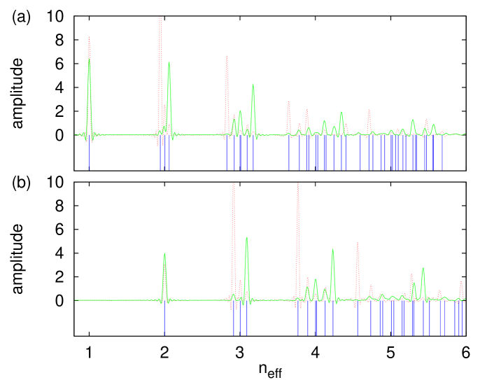
Figure 1: Spectra with (a) even and (b) odd $z$ parity of the Hamiltonian (2) with $\alpha=0.5$, $\beta=0.05$, $\zeta=0.01$ obtained from the propagation of two different 3D GWPs. Green and red line: ${\bf x}_{0}=(6,0,0)$, ${\bf p}_{0}=(0,\pm 1/\sqrt{2},1/\sqrt{2})$, respectively. The eigenvalues are extracted from the autocorrelation function by Fourier transform. The peak positions agree very well with the numerically exact eigenvalues of the effective quantum number marked by blue lines.

Once a time-dependent wave packet (11) is determined the eigenvalues $n_{\rm eff}$ of the stationary Schrödinger equation (2) and thus a quantum spectrum of the hydrogen atom in external fields can be obtained by frequency analysis of the time signal

$$C(\tau)=\langle\psi(0)|\psi(\tau)\rangle=\sum_{j}c_{j}e^{-2in_{\rm eff}^{(j)}\tau}\;,$$ (17)

with the amplitudes $c_{j}$ depending on the choice of the initial wave packet. In perpendicularly crossed fields the $z$ parity is conserved. Spectra with even and odd $z$ parity obtained from the Fourier transforms of the autocorrelation functions $C^{\pm}(\tau)=\langle\psi^{\pm}(0)|\psi^{\pm}(\tau)\rangle$ of the parity projected wave packets are shown in Fig. 1. The green and red lines result from the propagation of two different initial 3D GWPs with $\sigma=3.5$, $\epsilon=0.15$, the same initial position but different initial mean momenta. $N=41$ and $N=31$ basis states were coupled in the calculations. The line widths, i.e., the resolution of the spectra is determined by the length of the time signal $\tau_{\max}$. The eigenvalues obtained by numerically exact diagonalizations of the stationary Hamiltonian (2) are shown by the blue lines. The line-by-line comparison shows very good agreement between the exact spectrum and the results obtained from the wave packet propagation. The amplitudes of levels indicate the excitation strengths of states with higher or lower angular momentum $l_{z}$ by the two initial wave packets rotating clockwise or anticlockwise around the $z$-axis.

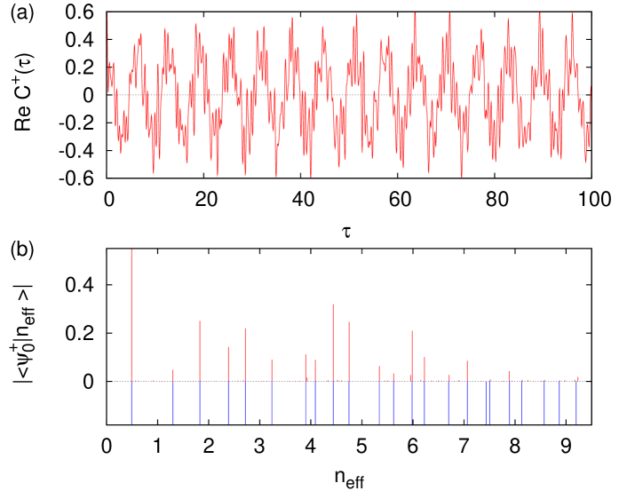
Figure 2: (a) Real part of the even $z$-parity autocorrelation function and (b) spectrum of the diamagnetic hydrogen atom extracted from the signal $C^{+}(\tau)$ by harmonic inversion at the field-free ionization threshold $E=0$, $\beta=n_{\rm eff}^{2}B=0.5$. For comparison the exact eigenvalues in (b) are marked by blue lines. They are in excellent agreement with the variational results (red lines).

The method presented can be especially adapted to systems with, e.g., cylindrical or spherical symmetries. For the hydrogen atom in a magnetic field we consider the very challenging regime around the field-free ionization threshold $E=0$ where the Coulomb and the Lorentz force are of comparable strength, resulting in a fully chaotic classical dynamics. The real part of the even $z$-parity autocorrelation function is shown in Fig. 2(a). A number of $N=90$ basis states was used in the computation. The eigenvalues are extracted from the signal $C^{+}(\tau)$ by the high-resolution harmonic inversion method [28] and drawn in Fig. 2(b). The agreement between the eigenvalues computed variationally (red lines) and the numerically exact results (blue lines) is very good. Some lines are lacking in the variational computation because of a nearly zero overlap of the respective eigenstates $|n_{\rm eff}\rangle$ and the initial GWP, but can be revealed by choosing different initial GWPs.

5 Conclusion

In this Letter we have extended the Gaussian wave packet method in such way that it can also be applied to quantum systems with singular Coulomb potentials. We have shown that the evolution in fitctious time can be calculated analytically in the pure quantum Coulomb problem. Therefore in applying the time-dependent variational principle to the description of time evolution of wave packets in perturbed atomic systems approximations arise only from the non-Coulombic parts of the potentials. The method can be adapted to special symmetries, such as axisymmetric or spherical, and opens the way to a wide range of applications in systems with Coulomb potentials.

References

- [1] J. E. Bayfield, P. M. Koch, Multiphoton ionization of highly excited hydrogen atoms, Phys. Rev. Lett. 33 (1974) 258–261.
- [2] E. J. Galvez, B. E. Sauer, L. Moorman, P. M. Koch, D. Richards, Microwave ionization of H atoms: Breakdown of classical dynamics for high frequencies, Phys. Rev. Lett. 61 (1988) 2011–2014.
- [3] H. Maeda, J. H. Gurian, T. F. Gallagher, Nondispersing Bohr wave packets, Phys. Rev. Lett. 102 (2009) 103001.
- [4] R. R. Jones, D. You, P. H. Bucksbaum, Ionization of Rydberg atoms by subpicosecond half-cycle electromagnetic pulses, Phys. Rev. Lett. 70 (1993) 1236–1239.
- [5] R. R. Jones, Creating and probing electronic wave packets using half-cycle pulses, Phys. Rev. Lett. 76 (1996) 3927–3930.
- [6] J. Parker, C. R. Stroud, Coherence and decay of Rydberg wave packets, Phys. Rev. Lett. 56 (1986) 716–719.
- [7] G. Alber, O. Zobay, Semiclassical interferences and catastrophes in the ionization of Rydberg atoms by half-cycle pulses, Phys. Rev. A 59 (1999) R3174–R3177.
- [8] M. Horbatsch, J. K. Liakos, Generation of harmonic radiation by hydrogen atoms in intense laser fields, Phys. Rev. A 45 (1992) 2019–2024.
- [9] E. J. Heller, Time-dependent approach to semiclassical dynamics, J. Chem. Phys. 62 (1975) 1544–1555.
- [10] E. J. Heller, Time dependent variational approach to semiclassical dynamics, J. Chem. Phys. 64 (1976) 63–73.
- [11] I. M. S. Barnes, M. Nauenberg, M. Nockleby, S. Tomsovic, Semiclassical theory of quantum propagation: The Coulomb potential, Phys. Rev. Lett. 71 (1993) 1961–1964.
- [12] I. M. S. Barnes, M. Nauenberg, M. Nockleby, S. Tomsovic, Classical orbits and semiclassical wavepacket propagation in the Coulomb potential, J. Phys. A 27 (1994) 3299–3321.
- [13] I. M. S. Barnes, Semiclassical wavepacket propagation in a hydrogen atom, Chaos, Solitons & Fractals 6 (1995) 531–537.
- [14] P. Kustaanheimo, E. Stiefel, Perturbation theory of Kepler motion based on spinor regularization, Journal für die reine und angewandte Mathematik 218 (1965) 204–219.
- [15] E. Stiefel, G. Scheifele, Linear and Regular Celestial Mechanics, Springer, 1971.
- [16] C. C. Gerry, Coherent states and the Kepler-Coulomb problem, Phys. Rev. A 33 (1986) 6–11.
- [17] T. Toyoda, S. Wakayama, Coherent states for the Kepler motion, Phys. Rev. A 59 (1999) 1021–1024.
- [18] B.-W. Xu, G.-H. Ding, Nonspreading coherent states for the hydrogen atom, Phys. Rev. A 62 (2000) 022106.
- [19] N. Unal, Parametric time-coherent states for the hydrogen atom, Phys. Rev. A 63 (2001) 052105.
- [20] S. A. Pol’shin, Coherent states for the hydrogen atom: discrete and continuous spectra, J. Phys. A 34 (2001) 11083–11094.
- [21] H. Friedrich, D. Wintgen, The hydrogen atom in a uniform magnetic field – An example of chaos, Phys. Rep. 183 (1989) 37–79.
- [22] H. Hasegawa, M. Robnik, G. Wunner, Classical and quantal chaos in the diamagnetic Kepler problem, Prog. Theor. Phys. Suppl. 98 (1989) 198–286.
- [23] T. Fabčič, J. Main, G. Wunner, Fictitious-time wave-packet dynamics: I. Nondispersive wave packets in the quantum Coulomb problem, Phys. Rev. A 79 (2009) 043416.
- [24] T. Fabčič, J. Main, G. Wunner, Fictitious-time wave-packet dynamics: II. Hydrogen atom in external fields, Phys. Rev. A 79 (2009) 043417.
- [25] A. D. McLachlan, A variational solution of the time-dependent Schrodinger equation, Mol. Phys. 8 (1964) 39–44.
- [26] S.-I. Sawada, R. Heather, B. Jackson, H. Metiu, A strategy for time dependent quantum mechanical calculations using a Gaussian wave packet representation of the wave function, J. Chem. Phys. 83 (1985) 3009–3027.
- [27] T. Fabčič, J. Main, G. Wunner, Time propagation of constrained coupled Gaussian wave packets, J. Chem. Phys. 128 (2008) 044116.
- [28] Dž. Belkić, P. A. Dando, J. Main, H. S. Taylor, Three novel high-resolution nonlinear methods for fast signal processing, J. Chem. Phys. 113 (2000) 6542–6556.