Clustering of K-band selected local galaxies

Abstract

We present detailed clustering analysis of a large K-band selected local galaxy sample, which is constructed from the 2MASS and the SDSS and consists of $82,486$ galaxies with $10<K<13.5$ and $0.01<z<0.1$. The two-point correlation function of the magnitude-limited sample in real space at small scales is well described by a power law $\xi(r)=(r/6.44\pm 0.23)^{-1.81\pm 0.02}$. The pairwise velocity dispersion is derived from the anisotropic two-point correlation function and find the dispersion $\sigma_{12}=685\pm 17\ {\rm km\,s^{-1}}$ if its scale invariance is assumed, which is larger than values measured in optical bands selected galaxy samples. We further investigate the dependence of the two-point correlation function and the $\sigma_{12}$ on the $g-r$ color and the $K$-band luminosity, obtain similar results to previous works in optical bands. Comparing a mock galaxy sample with our real data indicates that the semi-analytical model can not mimic the $\sigma_{12}$ in observation albeit it can approximate the two-point correlation function within measurement uncertainties.

1 Introduction

The track of galaxy formation and evolution keeps still one of the pivotal but intricate problems in modern astrophysical research. While there are large portion of prominent results mainly derived in optical bands, it is worth of addressing that observations of galaxies at distinct wave bands actually depict galaxies’ intrinsic properties in different aspects, which is essential to our attempt to an unbiased understanding of the formation and evolution of galaxies. The Near-Infrared (NIR) observation is of particular interests. A K-band $(2.15\mu m)$ selected galaxy sample has several advantages in studying galaxy. The K-correction in the K-band is a relatively small and better understood quantity comparing with the optical K-correction, galaxy’s K-band light is 5 – 10 times less sensitive to dust and stellar populations, and moreover is independent of galaxy spectral types at $z<1$ (e.g. Mobasher et al., 1986; Cowie et al., 1994). Therefore K-band observation enables a much homogeneous sampling of galaxy types. It is even advantageous that the K-band luminosity is tightly correlated with galaxy’s stellar mass, so that the analysis at K-band is a better probe of galaxy properties and relevant evolution history related to the stellar component than those measurements in B- and $r$-bands.

Studying clustering strength using the two-point correlation function (2PCF), of galaxies at different redshift bins is one of the most straightforward and effective methods of exploring how galaxy properties are related to the underlying dark matter distribution and henceforth to the macro history of galaxy formation and evolution. For example, the clustering of galaxies selected at $3.6\mu m$ with median redshift $z\sim 0.5$ offered by the Spitzer Wide-area Infrared Extragalactic (SWIRE) survey is directly compared to the results of local galaxy samples selected at K-band centered at $2.15\mu m$ (Waddington et al., 2007). Unfortunately in contrast with prolific photometric galaxy surveys available in NIR bands, spectroscopic information of these galaxies falls behind, it is not strange to see that majority of the clustering analysis of NIR galaxies resorts to angular correlation functions $\omega(\theta)$ (e.g. Baugh et al., 1996; McCracken et al., 2000; Roche et al., 2003; Waddington et al., 2007), the spatial correlation function $\xi(r)$ is applicable only occasionally (Carlberg et al., 1997).

In principle one can invert the angular 2PCF to the real space spatial correlation function through the Limber’s equation (see p. 194 of Peebles, 1980). The problem is the precision of the inversion relies significantly on the radial selection function of galaxies and the assumptions of small angle approximation and a power law $\xi(r)$, which introduces apparent uncertainties to its interpretation (Bernardeau et al., 2002), e.g. setting up the empirical evolution model of the real space two-point correlation function by $\xi(r,z)=(r/r_{0})^{-\gamma}\times(1+z)^{\gamma-3-\epsilon}$ (Phillipps et al., 1978).

Thanks to the Two-Micron All Sky Survey Extended Source Catalogue (2MASS XSC Jarrett et al., 2000) and the Sloan Digital Sky Survey (SDSS York et al., 2000), we are able to construct a large K-band selected local galaxy sample to measure spatial two point correlation function, and thus to built clustering reference of local NIR galaxies. By combining two-point correlation functions in both redshift and real spaces, we are also able to derive quantities on the galaxies’ peculiar velocities which are largely ignored in characterizing clustering of galaxies. Actually to appropriately descibe galaxy distribution, we should work in the phase space supported by both of the position and the peculiar velocity, especially in the nonlinear regime. Thus measurement of the pairwise peculiar velocity dispersion is robust, providing an important statistics to identify galaxy populations and test galaxy formation models (e.g. Zhao et al., 2002; Yoshikawa et al., 2003; Jing & Börner, 2004; Slosar et al., 2006; Li et al., 2007).

A brief summary of the sample used is presented in Section 2, as well as the estimation method of 2PCF, including technical issues such as random sample construction, correction to the fibre collision. In Section 3 we present measurements of the full, flux-limited sample in both redshift- and real-spaces, in together with the redshift-space distortion parameter and the pairwise velocity dispersion. In Section 4 the full sample is divided into different sub-samples according to their color and luminosity to probe the clustering as functions of these properties.

Throughout this paper, galaxy distances are obtained from redshifts assuming a cosmology with $\Omega_{m}=0.3,\Omega_{\Lambda}=0.7$, quoted in units of $\,h^{-1}{\rm Mpc}$. Absolute magnitudes quoted for galaxies assume $h=1$ to avoid the $-5\log_{10}h$ factor.

2 Samples and estimation procedure

2.1 the K-band sample of local galaxies

Our K-band galaxy sample is selected from the 2MASS XSC. Redshifts for this smaple are obtained from the SDSS. The two catalogues actually have been combined by Blanton et al. (2005) into the New York University Value-Added Galaxy Catalog (NYU-VAGC) to form a local redshift sample(mostly below $z\sim 0.3$) , with a coverage of 9938 $deg^{2}$ for photometric imaging and 6750 $deg^{2}$ for spectroscopic observation.

The completeness of the cross-matched 2MASS+SDSS Catalogue has been extensively discussed (e.g. Bell et al., 2003). Following these practices, we select the galaxies by the extinction-corrected Kron magnitudes in the range $10\leq K\leq 13.5$, and redshifts in the range $0.01\leq z\leq 0.1$. In the apparent magnitude limits adopted here, the bright end is chosen to avoid incompleteness due to the large angular sizes of galaxies, while the faint end is such to match the magnitude limit of 2MASS. We also use a low redshift cut rejects galaxies with redshifts seriously affected by Hubble flow. The final flux-limited sample, our main sample, accumulates 78,339 galaxies with redshifts in total, with a median redshift $\sim 0.06$.

Figure 1: The K-corrected g - r color vs. K-band absolute magnitude for all galaxies. The vertical line demarcates a simple cut at g - r = 0.7

Table 1: The K-selected samples including both red and blue populations. All samples are in the range of $10<K<13.5$ and $0.01<z<0.1$. $M^{*}$ and $\alpha$ are fitted parameters of the Schechter luminosity function (Schechter, 1976). $r_{0}$ and $\gamma$ are obtained from fit to the projected 2PCF $w_{p}(\sigma)$. The numbers of galaxies quoted here include those lack of redshift due to fibre collision.

label	$N_{\mathrm{gal}}$	$M^{*}$	$\alpha$	$r_{0}(\,h^{-1}{\rm Mpc})$	$\gamma$	$\beta$
Main	82,486	-23.38	-0.94	6.44 $\pm$ 0.23	1.81 $\pm$ 0.02	0.39 $\pm$ 0.17
Red	46,689	-23.31	-0.48	7.62 $\pm$ 0.32	1.87 $\pm$ 0.03	0.35 $\pm$ 0.20
Blue	35,797	-23.08	-1.11	4.92 $\pm$ 0.14	1.67 $\pm$ 0.02	0.50 $\pm$ 0.15

The K-selected sample is further divided into two sub-samples according to their SDSS color $(g-r)$: the blue sample with $(g-r)<0.7$ and red sample with of $(g-r)>0.7$ (Figure 1 and Table 1). Both red and blue samples have similar space densities, but galaxies in the red sample are systematically more luminous and therefore mainly inhabit at higher redshift: the median redshift of red galaxies is $z_{med}\sim 0.065$ whereas for the blue $z_{med}\sim 0.054$.

A set of volume-limited sub-samples within different absolute magnitude bins are also constructed for analysis (Table 2).

Table 2: Volume-limited sub-samples and their 2PCF parameters. ${\bar{n}}$ is the mean number density in unit of $10^{-3}h^{3}{\rm Mpc}^{-3}$, and $r_{0}$ is in unit of $\,h^{-1}{\rm Mpc}$. All galaxy samples are of $10<K<13.5$, $0.01<z<0.1$. $r_{0}$ and $\gamma$ are obtained from $w_{p}(\sigma)$, the numbers in parentheses are values of corresponding luminosity sub-samples of the mock galaxy catalogue.

Abs. Mag.	Redshift range	$N_{\mathrm{gal}}$	${\bar{n}}$	$r_{0}$	$\gamma$
-25 – -24	0.033 – 0.100	14,152	0.87	$7.17\pm 0.30$ ($6.93\pm 1.10$)	$1.87\pm 0.03$ ($1.82\pm 0.07$)
-24 – -23	0.021 – 0.067	19,714	3.83	$5.52\pm 0.28$ ($4.97\pm 0.23$)	$1.83\pm 0.03$ ($1.87\pm 0.03$)
-23 – -22	0.013 – 0.042	8,969	7.08	$5.23\pm 0.65$ ($4.50\pm 0.24$)	$1.83\pm 0.04$ ($1.86\pm 0.04$)
-22 – -21	0.010 – 0.026	2,232	7.19	$4.46\pm 0.57$ ($4.79\pm 0.29$)	$1.86\pm 0.10$ ($1.92\pm 0.04$)

2.2 mock galaxy catalogue

We also compare our sample with a mock galaxy catalogue to scout for the performance of semi-analytical models for hierarchical galaxy formation (see Baugh, 2006, and references there in). The mock catalogue is derived from a high-resolution pure dark matter cosmological simulation with $512^{3}$ particles in a box of size $100\,h^{-1}{\rm Mpc}$ run by the GADGET2 code (Springel, 2005). The fundamental cosmological parameters for the simulation are set as $\Omega_{\Lambda}=0.762,\ \Omega_{m}=0.238,\ h=0.73,\ \sigma_{8}=0.74,\ n=1$, rest simulation parameters are the same as those in the pure dark matter run by Lin et al. (2006), e.g. the particle mass is $5.5\times 10^{8}h^{-1}M_{\sun}$ and the soft length is $4.5h^{-1}{\rm kpc}$. We generate the mock galaxies at $z=0.05$ from the output of the simulation by the semi-analytical model of Kang et al. (2005). Luminosities are the only derived property for the mock galaxies, thus we divide the mock galaxies into a set of luminosities bins and study galaxy and dark halo properties in each bin.

2.3 estimation of the two-point correlation functions

Two types of 2PCFs for this sample are measured to capture the clustering patterns: one is the isotropic $\xi(s)$ with $s$ denoting the separation of a pair of galaxies in redshift space, and the other is the two-dimensional function $\xi(\sigma,\pi=\sqrt{s^{2}-\sigma^{2}})$ with $\pi$ indicating the separation of a pair of galaxies parallel to the line-of-sight and the $\sigma$ being the separation perpendicular to the line-of-sight. The latter is mainly utilised to obtain the redshift distortion free function, the projected 2PCF $w_{p}(\sigma)=\int\xi(\sigma,\pi){\rm d}\pi$, and consequently the real space function $\xi(r)$ after proper inversion (e.g. Davis & Peebles, 1983; Hawkins et al., 2003).

The 2PCFs are measured using the estimator of Landy & Szalay (1993),

$$\xi=\frac{DD-2DR+RR}{RR}\ ,$$ (1)

in which $DD$ is the normalised number of weighted galaxy-galaxy pairs at given separation, $RR$ is the normalised number of random-random pairs within the same separation in the random catalogue and $DR$ is the normalised number of weighted galaxy-random pairs. In general the scale $s$ of $\xi(s)$ is binned uniformly in logarithm scale, and for $\xi(\sigma,\pi)$, $\sigma$ and $\pi$ are binned in linear scale.

To proceed the estimation with Eq. 1, an auxiliary sample of completely random points in the exactly the same geometric window as the galaxy sample is prerequisite. The random samples should have the same redshift, magnitude and mask constraints as the real data, with a smooth selection function matching the $N(z)$ of the real data. The luminosity functions of the flux-limited samples, used to generate the selection function, are computed with the STY method (Sandage et al., 1979) in form of the Schechter function (Table 1). We generate a random sample ten times larger than the observed K-selected sample, and the random samples for red and blue samples are 15 times larger than observed ones.

A weight is assigned to each galaxy and random point according to their redshift and angular position to minimize the variance in estimated $\xi$ (Efstathiou, 1988; Hamilton, 1993),

$$\omega_{i}=\frac{1}{1+4\pi\,n(z)\Phi_{i}\,J_{3}(s)}\ ,$$ (2)

where $\Phi_{i}$ is the selection function at the location of $i$th galaxy, $n(z)$ is the mean number density, and $J_{3}(s)=\int_{0}^{s}\xi(s)s^{2}ds$. The $J_{3}(s)$ is computed using a power-law $\xi(s)$ with correlation length $s_{0}=12\,h^{-1}{\rm Mpc}$ and $\gamma_{0}=1$, we find that the difference between our estimate and that using a raw measured $\xi(s)$ is negligible, in agreement with the conclusion of Hawkins et al. (2003). To normalize the pair counts properly, we assure that the sum of weights of the random catalogue equal the sum of weights of the real galaxy catalogue, both are a function of scale.

We need to correct the incompleteness in the spectroscopic sample due to the effect of collided fiber constraints. The design of the SDSS instrument means that fibers can not be placed closer than 55 arcsec on the same tile, members of a close pair of galaxies cannot be targeted in a single fibre configuration so that the survey misses a large fraction of close pairs. Because 2PCF will be systematically underestimated without taking account of fiber collisions effect, several methods are developed to correct this bias (Zehavi et al., 2002; Hawkins et al., 2003). We adopt the method of Zehavi et al. (2002) by assigning the redshift of the observed galaxy in a pair to the pair member whose redshift was absent. Then we obtain “collision corrected” redshift. At large scales, where both members of the pair contribute to the same separation bin, this method is equivalent to double weighting. We argue this method should perform better on small scales because it retains information about the known angular positions. Zehavi et al. (2005) showed that this method is an adequate treatment: residual systematics for the redshift space correlation function were considerably smaller than the statistical errors, and this was even more true for the projected 2PCF $w_{p}(\sigma)$.

The covariance matrix is computed with the jack-knife technique (Lupton, 1993; Zehavi et al., 2002), the galaxy sample is splitted into thirty separate regions of approximately equal sky area, and then we perform the analysis thirty times, each time leaving a different region out. The estimated statistical covariance of 2PCF measured in two bins of $i$ and $j$ is then

$${\rm Cov}(\xi_{i},\xi_{j})=\frac{N-1}{N}\sum_{\ell=1}^{N}(\xi_{i,\ell}-\overline{\xi_{i}})(\xi_{j,\ell}-\overline{\xi_{j}})\ ,$$ (3)

in which $N$ is the number of jack-knife sub-samples.

3 Clustering of the main sample

3.1 2PCF in redshift space

The first one we calculated is the 2PCF $\xi(s)$ for the main sample from $s=0.01\,h^{-1}{\rm Mpc}$ to $s=100\,h^{-1}{\rm Mpc}$ in redshift space. $s$ is divided into equally logarithmic bins of width $\Delta\log_{10}(s/\,h^{-1}{\rm Mpc})=0.125$. $\xi(s)$ is not a single power law at all scales (Figure 2), rather

$$\xi(s)=(\frac{s}{s_{0}})^{-\gamma_{s}},\ \ (s_{0},\gamma_{s})=\begin{aligned} &(11.69\pm 0.89,0.98\pm 0.02),\ if\ s\in(0.1,3)\ ;\\ &(7.64\pm 0.41,1.60\pm 0.05),\ if\ s\in(3,10)\ .\end{aligned}$$ (4)

It is known that $\xi(s)$ also consists of the contribution from the galaxy peculiar velocities causing the redshift distortion, in addition to the true spatial correlation of galaxies (Kaiser, 1987; Hamilton, 1998). Thus we need to break the degeneracy between the spatial clustering and the velocity correlation before making direct comparison of $\xi(s)$ in different redshift bins.

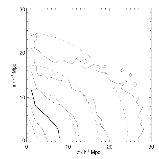
Figure 2: 2PCFs of the main sample. Top-left: $\xi$ in redshift space, the dot-dashed line is the power law at scales $0.1<s<3\,h^{-1}{\rm Mpc}$ and the dashed line is the fit at scales $3<s<10\,h^{-1}{\rm Mpc}$ (Eq. 4). Top-right: $\xi(\sigma,\pi)$ contours, $\sigma$ and $\pi$ are separations perpendicular and parallel to the line of sight respectively, solid contours are measurements at levels of $4,2,1,0.5,0.25,0.125$ outwards and dotted lines are the isotropic 2PCF expected in the absence of redshift-space distortion. Bottom-left: projected 2PCF $w_{p}(\sigma)$(solid points), the solid line is the power law fit. Bottom-right: 2PCF $\xi(r)$ in real space inverted from $w_{p}$ through Eq. 7, solid line is the power law transformed from the fit to the $w_{p}$ on the left. Error bars in these plots are the $1\sigma$ scatters of jackknife sub-samples.

3.2 The projected 2PCF

Galaxy’s peculiar motion only cause drifting of the radial position. To minimize this effect, we can calculate the correlation function as a function of $\sigma$ and $\pi$, where $\sigma$ is perpendicular to the line-of-sight and $\pi$ is parallel to the line-of-sight. Then the projection of $\xi(\sigma,\pi)$ onto the $\sigma$ plane is independent to redshift space distortion and gives the information of real space correlation function.

The effect of redshift distortion is clearly seen in the $\xi(\sigma,\pi)$ contour of the main sample in Figure 2: the contours are elongated along the line-of-sight direction at small $\sigma$ separation, exhibiting the phenomenon of fingers-of-God by the random pairwise velocity; at large $\sigma$ scales, the contours are squashed in the $\pi$ direction due to gravitational coherent inflow (Hawkins et al., 2003).

Integrating the anisotropic $\xi(\sigma,\pi)$ over $\pi$ gives the projected 2PCF,

$$w_{p}(\sigma)=\int_{-\pi_{max}}^{+\pi_{max}}\xi(\sigma,\pi)d\pi=\sum_{i}\xi(\sigma,\pi_{i})\Delta{\pi_{i}}\ ,$$ (5)

which has practically an upper limit $\pi_{max}=50\,h^{-1}{\rm Mpc}$. We tested that there is little difference if using a larger cutoff.

$w_{p}$ is related to the 2PCF in real space through the Abel transform (Davis & Peebles, 1983)

$$w_{p}(\sigma)=2\int_{\sigma}^{\infty}\frac{r\xi(r)\,dr}{\sqrt{r^{2}-\sigma^{2}}}\ ,$$ (6)

where the inversion renders $\xi(r)$ assuming a step function-like $w_{p}(\sigma)=w_{i}$ at each bin centered at $\sigma_{i}$

$$\xi(\sigma_{i})=\frac{1}{\pi}\sum_{j\geq i}\frac{w_{j+1}-w_{j}}{\sigma_{j+1}-\sigma_{j}}\ln\left(\frac{\sigma_{j+1}+\sqrt{\sigma^{2}_{j+1}-\sigma_{i}^{2}}}{\sigma_{j}+\sqrt{\sigma_{j}^{2}-\sigma_{i}^{2}}}\right)$$ (7)

for $r=\sigma_{i}$ (Saunders et al., 1992). Mathematically the inversion is not stable but in practice works well in $r<30\,h^{-1}{\rm Mpc}$. If we simply assume $\xi(r)=(r/r_{0})^{-\gamma}$ , the integral in Eq. 6 can be done analytically, yielding

$$w_{p}=A\sigma^{1-\gamma},\ with\ A=r_{0}^{\gamma}\Gamma(\frac{1}{2})\Gamma(\frac{\gamma-1}{2})/\Gamma(\frac{\gamma}{2}),$$ (8)

where $\Gamma$ is the Gamma function. It is true that $w_{p}$ for our main sample is a power law function at small scales (Figure 2), the best-fit parameters are $\gamma=1.81\pm 0.02$ and $r_{0}=6.44\pm 0.23$ in the regime of $0.1\,h^{-1}{\rm Mpc}<\sigma<18\,h^{-1}{\rm Mpc}$.

Table 3 lists the results of our K-selected sample and those selected in the other bands for comparison: $b_{J}$ of 2dFGRS and $r$ of SDSS. We conclude that the correlation function will have larger amplitude and steeper slope if the galaxies are selected at longer wavelength band.

Table 3: Clustering of galaxies selected at different bands. $r$-band (SDSS) result comes from Zehavi et al. (2002, 2005) and the $b_{J}$-band (2dFGRS) is given by Hawkins et al. (2003).

band	$N_{\mathrm{gal}}$	$r_{0}$ ($\,h^{-1}{\rm Mpc}$)	$\gamma$	$\sigma_{12}$ ($\ {\rm km\,s^{-1}}$)
Ks	82,486	6.44 $\pm$ 0.23	1.81 $\pm$ 0.02	685 $\pm$ 17
r	154,014	5.59 $\pm$ 0.11	1.84 $\pm$ 0.01	640 $\pm$ 60
$b_{J}$	165,659	4.95 $\pm$ 0.27	1.72 $\pm$ 0.04	506 $\pm$ 52

3.3 the pairwise velocity dispersion

Currently there is no precise theory on the full scale range redshift distortion (Scoccimarro, 2004). But we can still approach to this topic with reasonable assumptions. Intuitively redshift distortion can be approximated by certain convolution of two components dominated in different regimes, coherent infall is responsible for the clustering enhancement at large scales while the smearing of correlation strength at small scales is attributed to random motions.

Kaiser (1987) found that at large scales the boost to the power spectrum by the peculiar velocities takes a particularly simple form, which was later completed and translated to the real space by Hamilton (1992),

$$\xi^{\prime}(\sigma,\pi)=\xi_{0}(s)P_{0}(\mu)+\xi_{2}(s)P_{2}(\mu)+\xi_{4}(s)P_{4}(\mu)\ ,$$ (9)

where $P_{\ell}(\mu)$ is Legendre polynomials, $\mu=\cos(\theta)$ with $\theta$ being the angle between $r$ and $\pi$. Assuming $\xi=(r/r_{0})^{-\gamma}$ then renders

$$\xi_{0}(s) =\xi(s)=\left(1+\frac{2\beta}{3}+\frac{\beta^{2}}{5}\right)\xi(r)$$ (10)

$$\xi_{2}(s) =\left(\frac{4\beta}{3}+\frac{4\beta^{2}}{7}\right)\left(\frac{\gamma}{\gamma-3}\right)\xi(r)$$

$$\xi_{4}(s) =\frac{8\beta^{2}}{35}\left(\frac{\gamma(2+\gamma)}{(3-\gamma)(5-\gamma)}\right)\xi(r)\ ,$$

where $s$ and $r$ have the correspondent values, $\beta$ is the linear redshift distortion parameter, $\beta\approx\Omega_{0}^{0.6}/b$, and $b$ is the linear bias parameter. The first equation is independent on the form of $\xi(r)$.

To incorporate effects of random motion, the anisotropic 2PCF in redshift space is then approximated by the convolution of the $\xi^{\prime}(\sigma,\pi)$ by Eq. 9 with the distribution function of the pairwise velocity $f(v_{12})$ (c.f. Peebles, 1993),

$$\xi(\sigma,\pi)=\int_{-\infty}^{+\infty}\xi^{\prime}(\sigma,\pi-\frac{v_{12}}{H_{0}})f(v_{12})dv_{12}\ ,$$ (11)

and in general $f(v_{12})$ is assumed to be an exponential distribution of dispersion $\sigma_{12}$

$$f(v_{12})=\frac{1}{\sigma_{12}\sqrt{2}}\exp\left(-\frac{\sqrt{2}v_{12}}{\sigma_{12}}\right)\ .$$ (12)

After measuring $\xi(s)$ and $\xi(r)$ at large scales, we can obtain the redshift distortion parameter $\beta$ via the first equation in Eq. 10 easily. Then we combine Eq. 9 – Eq. 12 to fit the $\xi(\sigma,\pi)$ data grid to determine other model parameters. However there are implicit assumptions in the prescription: (1) the linear bias parameter $b$ is forced to be scale-independent; (2) the pairwise velocity dispersion $\sigma_{12}$ is presumed invariant to the separation $\pi$ along the line-of-sight but could be a function of the perpendicular separation $\sigma$. Therefore the resulting $\sigma_{12}$ in the model is not the actual true pairwise velocity dispersion. To have meaningful comparison with simulations, we need to estimate the $\sigma_{12}$ from the 2PCFs of the simulation data in the same way as of the galaxy sample.

Figure 3 shows the ratio of the redshift-space 2PCF to the real-space 2PCF, and the derived $\sigma_{12}$ as function of $\sigma$. $\xi(s)/\xi(r)$ increases with scales, and becomes roughly constant in the range $4\,h^{-1}{\rm Mpc}<r<13\,h^{-1}{\rm Mpc}$ as expected, however, the ratio increases again at larger scales. If we exclude the galaxies in the Sloan Great Wall region ($11^{h}<{\rm R.A.}<14^{h}$), the $\xi(s)/\xi(r)$ ratio indeed does not show the up-shooting anymore. Nevertheless, there are no appealing arguments about whether chopping off galaxies in the Sloan Great Wall guarantees fairness, we just pick up points in the scale range $(4,13\,h^{-1}{\rm Mpc})$ to fit to a constant and get $\xi(s)/\xi(r)=1.29\pm 0.14$, or $\beta=0.39\pm 0.17$, considering the fact that the final $\sigma_{12}$ is not sensitive to the $\beta$ at all (Li et al., 2006a).

Figure 3: Left: ratios of $\xi(s)/\xi(r)$ of the full sample (solid circles) in comparison with that of the sample without the Sloan Great Wall (open triangle), the dotted line corresponds to $\beta=0.39$. Right: the derived pairwise velocity dispersion $\sigma_{12}(\sigma)$. Error bars are obtained by jackknife re-sampling.

The $\sigma_{12}$ as a function of projected separation $\sigma$ shown in Fig. 3 has a classical shape as many other measurements (e.g. Jing & Börner, 2004; Li et al., 2007): $\sigma_{12}$ rises from $650\ {\rm km\,s^{-1}}$ up to $750\ {\rm km\,s^{-1}}$ as $\sigma$ increases from $0.1\,h^{-1}{\rm Mpc}$ to $0.3\,h^{-1}{\rm Mpc}$, forms a plateau till to $\sigma\sim 1\,h^{-1}{\rm Mpc}$, then drops down again at larger scales. If a scale independent $\sigma_{12}$ is assumed, the best fitted $\sigma_{12}=685\pm 17\ {\rm km\,s^{-1}}$ within $0.1\,h^{-1}{\rm Mpc}<r<18\,h^{-1}{\rm Mpc}$. Our $\sigma_{12}$ are significantly higher than that of $b_{J}$-band sample (2dFGRS, Hawkins et al., 2003) and slightly larger than the $r$-band sample (SDSS, Zehavi et al., 2002).

4 color sub-samples

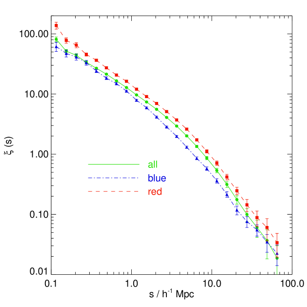
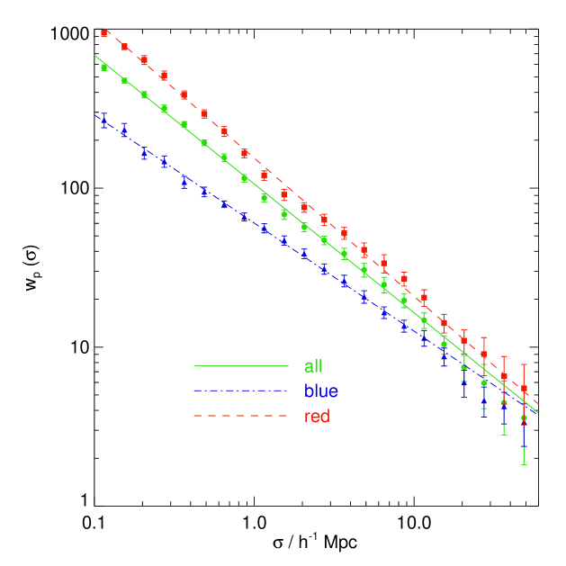
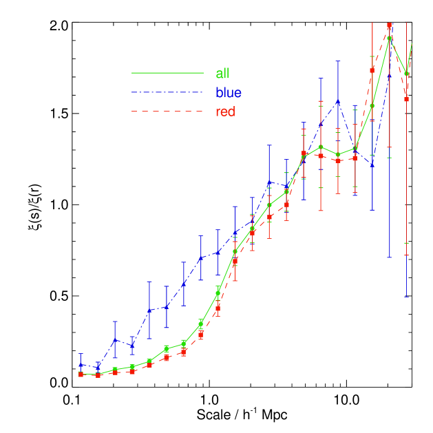
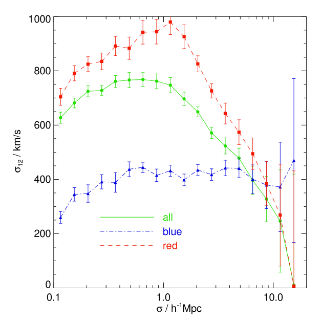
Figure 4: $g-r$ color dependence of 2PCFs and $\sigma_{12}$. All error bars are derived from jackknife sub-samples.

Figure 4 displays the clustering dependence on the color of galaxies, from $\xi(s)$ and $w_{p}$ as numerous works already revealed that spatial clustering for red galaxies is much stronger than for blue galaxies (see also Table 1). The slope of the 2PCF is a direct indicator of strength of the galaxy dynamic non-linearity, thus red galaxies with steeper 2PCF are more harassed by the gravitational turbulence at small scales or local structures than blue galaxies. In the scheme of halo models, the slope of 2PCF is determined by the percentage of contribution from the one-halo term and two-halo terms, rather than the mass of the halo in which the galaxy resides (Cooray & Sheth, 2002). A steeper 2PCF at small scales contains more power from the one-halo term. If galaxies are simply centrals and satellites in dark halo, it leads to a conclusion that the satellite fraction in the red sub-sample is higher than in the blue sub-sample, although red galaxies incline to occupy more massive halos than blue galaxies. In fact the interpretation is confirmed by the velocity information: $\sigma_{12}(\sigma)$ of blue galaxies is very flat and has much lower amplitude than red galaxies over wide range of projected separation, which is exactly what is observed in simulations when reducing satellite fraction in mock galaxy samples (Slosar et al., 2006). We also note that the color dependence of $\sigma_{12}$ is very similar to the simulation results of the old and young populations galaxies demonstrated by Weinberg et al. (2004).

5 volume-limited sub-samples and comparison with mock catalogue

We construct four volume-limited sub-samples to investigate the luminosity dependence of clustering (Table 2). The main sample is divided to 4 absolute magnitude bins centered approximately from $M^{*}+2$ to $M^{*}-1$, where $M^{*}=-23.38$ is the characteristic luminosity of the Schechter function (Schechter, 1976). The number density for galaxies in the lowest luminosity bin is 8 times higher than that in the highest luminosity bin.

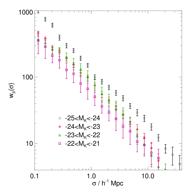
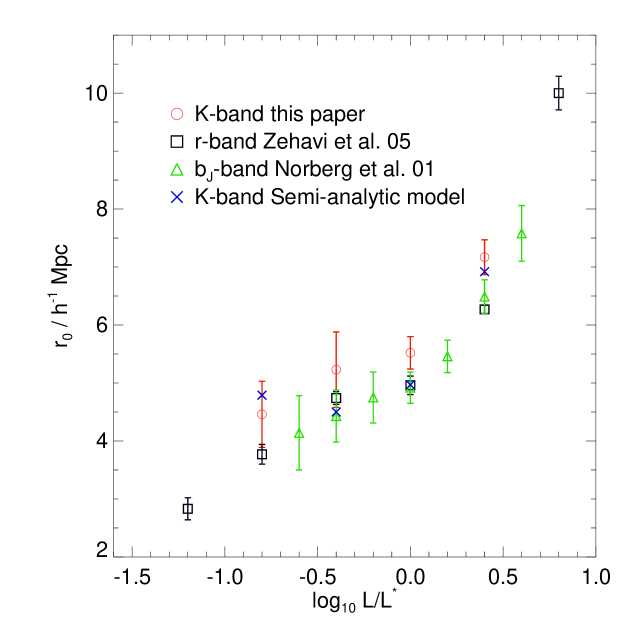
Figure 5: Top: projected correlation functions $w_{p}(\sigma)$ for the volume-limited sub-samples. Bottom: luminosity dependence of the comoving correlation lengths and the linear bias parameters of different galaxy samples and the mock galaxy sample. The relative bias factors $b/b^{*}$ is defined by the amplitude of $w_{p}(\sigma)$ measured at $\sigma=2.7\,h^{-1}{\rm Mpc}$ divided by the same quantity of the $-24<M_{K}<-23$ sub-sample ($L\approx L^{*}$), the dotted curve is at the $b_{J}$-band of the 2dFGRS survey $b/b^{*}=0.85+0.15L/L^{*}$ (Norberg et al., 2001), the solid curve is from the SDSS $r$-band power spectrum $b/b^{*}=0.85+0.15L/L^{*}-0.04(M-M^{*}$) (Tegmark et al., 2004), and the dashed curve is a fit to the $w_{p}(\sigma)$ of stellar mass sub-samples $b/b^{*}=0.896+0.097M/M^{*}$ (Li et al., 2006b) in which $M$ and $M^{*}$ refer to stellar mass.

Figure 5 shows the projected correlation functions $w_{p}(\sigma)$ of volume-limited samples, and Table 2 lists the parameters $r_{0}$ and $\gamma$ for power law $\xi(r)$ models by fitting $w_{p}(r_{p})$ in the range $0.1\,h^{-1}{\rm Mpc}<\sigma<13\,h^{-1}{\rm Mpc}$. The slopes of these sub-samples are roughly constant with errorbars, indicating weak dependence on luminosity; but the correlation length $r_{0}$ does increase with luminosity, thus being consistent with earlier studies (Norberg et al., 2001; Zehavi et al., 2005; Li et al., 2006b), and the $r_{0}$ – $L$ relation follows the same law as the relations in other bands and simulations (Figure 5).

We also explore the relative bias factor $b/b^{*}$ computed using the ratio of the $w_{p}(2.7\,h^{-1}{\rm Mpc})$ of our four sub-samples to the $w_{p}(2.7\,h^{-1}{\rm Mpc})$ of the $-24<M_{K}<-23$ sub-sample ($L\approx L^{*}$). This fiducial separation of $2.7\,h^{-1}{\rm Mpc}$ is chosen because it is well out of the extremely non-linear regime, but still small enough so that the correlation functions are very accurately measured for all sub-samples. In the bottom right panel of Figure 5, we compared our measured $b/b^{*}$ to the models of Norberg et al. (2001), Tegmark et al. (2004) and Li et al. (2006b) together with data from simulations. Within the estimated uncertainties, the models of Norberg et al. (2001) and Tegmark et al. (2004) are basically consistent with our estimations, but the model of Li et al. (2006b) and the semi-analytical model fail to produce enough clustering power in the highest luminosity bin.

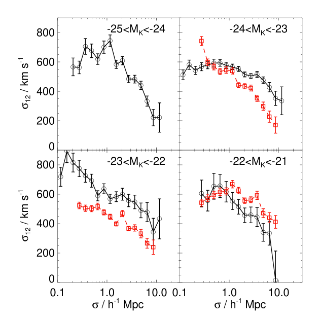
Figure 6: $\sigma_{12}$ of volume limited sub-samples (circles) against semi-analytical modelling (squares).

The luminosity dependence of $\sigma_{12}$ is rather much complicated as already realized by Jing & Börner (2004) and Li et al. (2006a). It is pointed out that, at small separation, $\sigma_{12}$ has a trough at $L^{*}$, becomes relative flat at lower luminosity end and increasing rapidly at $L>L^{*}$. This has not been reproduced by any current halo models. Figure 6 shows that the $\sigma_{12}$ curve of $L^{*}$ sub-sample at $\sigma<1\,h^{-1}{\rm Mpc}$ is fairly flat and has smaller amplitude than other luminosity sub-samples, implying a relative smaller fraction of satellites within the luminosity bin or the stellar mass range. Interestingly that $\sigma_{12}$ curves of the brightest sub-sample and the faintest sub-sample have very similar shape although amplitudes differ slightly, it seems that the two sub-samples contain similar fraction of satellites although their occupied halos have very different masses, since the brightest sub-sample has a much bigger bias than the faintest sub-sample.

The semi-analytical model works well for galaxies with low K-band luminosity, but displays significant discrepancies at high luminosity end despite the rough agreement in spatial clustering (Table 2). The case in K-band is different to the discovery of Li et al. (2007) at $r$-band where there are less differences between the semi-analytical model and the data at lower luminosity end. However the inconsistency of the semi-analytical model may be cuased by the limited size of the simulation, henceforth deficiency in large mass halos to provide sufficient number of galaxies of high stellar masses.

6 summary and discussion

For furnishing the clustering evolution of NIR galaxies, a local galaxy catalogue limited by K-band magnitudes of $10<K<13.5$ is generated by cross-matching the 2MASS data with the SDSS survey, then we carefully measured the 2PCFs and the pairwise velocity dispersion of the galaxy sample, as well as their color and luminosity dependence respectively.

In the redshift space, the 2PCF $\xi(s)$ of the flux-limited sample complies with shallower power law at scales of $s<\sim 3\,h^{-1}{\rm Mpc}$ than that at larger scales, but in real space the 2PCF $\xi(r)$ derived from the projected 2PCF $w(\sigma)$ is perfectly approximated by a single power law with $r_{0}=6.44\pm 0.23\,h^{-1}{\rm Mpc}$ and $\gamma=1.81\pm 0.02$ for $r<1\sim 10\,h^{-1}{\rm Mpc}$ (Figure 2). The estimated correlation length supports the conclusion of Waddington et al. (2007) that the clustering of NIR galaxies evolves very slow upto $z\sim 0.5$. The pairwise velocity dispersion at small scales is directly related to the spatial distribution in the halo (Slosar et al., 2006), our $\sigma_{12}$ of local NIR galaxies has shape analogous to those found in simulations, showing a bump at scales around $1\,h^{-1}{\rm Mpc}$, but is larger than in optical bands, being $685\pm 17\ {\rm km\,s^{-1}}$ if assuming scale invariant $\sigma_{12}$ (Table 3). The phenomenon could be rooted in different luminosity functions at these bands, it is likely that the distribution of $K$-band luminosity or stellar mass of satellite galaxies is more concentrated in the range defining our sample than that of central galaxies. Regrettably we do not have a large NIR galaxy sample at high redshift with redshift, otherwise comparison of $\sigma_{12}$ would enable us peering into the evolution of the positioning of NIR galaxies in their host halos, or the velocity biasing of galaxies relative to the dark matter.

The optical color dependence of the clustering of NIR galaxies is similar to optical bands selected galaxies, blue galaxies of $g-r<0.7$ are much less clustered than red galaxies, and displaying a very flat and low $\sigma_{12}$ in nonlinear regime as consequences of having smaller fraction of satellite galaxies. And the luminosity dependence of 2PCF and $\sigma_{12}$ of our NIR galaxies is not different with that of optical galaxies in spite of the very different luminosity functions. As the $K$-band luminosity is tightly correlated with the stellar mass, it is somehow surprising to discover that the empirical formula of relative biasing by stellar mass in Li et al. (2006b) under-predict the bias of the brightest volume-limited sample. Also, the transition of the shape and amplitude of $\sigma_{12}$ at $L^{*}$ might infer that the luminosity distribution of satellite galaxies in low mass halos are very different to that in high mass halos.

Examination of our galaxy sample against mock galaxy sample reveals that the $K$-band luminosity dependence of the 2PCF can be approximately reproduced by semi-analytical modelling within measurement errors, but the $\sigma_{12}$ of the mock deviates from observation significantly in aspects of amplitude, shape and luminosity dependence, especially for bright galaxies. The peculiar velocity of galaxy is a conundrum in galaxy formation models both in theories and simulations, accurate modelling requires exquisite fabrication of galaxies in halos and corresponding evolution paths, it seems so far there is still a long way to go.