.

The role of a delay time on the spatial structure of chaotically advected reactive scalars

Abstract

The stationary-state spatial structure of reacting scalar fields, chaotically advected by a two-dimensional large-scale flow, is examined for the case for which the reaction equations contain delay terms. Previous theoretical investigations have shown that, in the absence of delay terms and in a regime where diffusion can be neglected (large Péclet number), the emergent spatial structures are filamental and characterized by a single scaling regime with a Hölder exponent that depends on the rate of convergence of the reactive processes and the strength of the stirring measured by the average stretching rate. In the presence of delay terms, we show that for sufficiently small scales all interacting fields should share the same spatial structure, as found in the absence of delay terms. Depending on the strength of the stirring and the magnitude of the delay time, two further scaling regimes that are unique to the delay system may appear at intermediate length scales. An expression for the transition length scale dividing small-scale and intermediate-scale regimes is obtained and the scaling behavior of the scalar field is explained. The theoretical results are illustrated by numerical calculations for two types of reaction models, both based on delay differential equations, coupled to a two-dimensional chaotic advection flow. The first corresponds to a single reactive scalar and the second to a nonlinear biological model that includes nutrients, phytoplankton and zooplankton. As in the no-delay case, the presence of asymmetrical couplings among the biological species results in a non-generic scaling behavior.

1 Introduction

The transport and stirring of reactive scalars is a problem that naturally arises in many environmental and geophysical situations as well as in engineering applications. Important examples of reactive scalars may be found in oceanic ecosystems e.g. interacting nutrient and plankton populations, in atmospheric chemistry e.g. stratospheric ozone as well as in microfluidics and combustion. In all of these examples, fine-scale strongly-inhomogeneous structures, usually in the form of filaments, characterize the spatial structure of the corresponding reactive scalar fields [2, 26, 29, 35, 33, 17]. Understanding the main mechanisms controlling the nature of these small-scale structures is important as they can have a large-scale impact for instance on the global ozone depletion [12] or on the total plankton production [21].

It is now well known that small-scale filamentary structures arise naturally through chaotic advection in spatially smooth (differentiable) and time-dependent velocity fields [3, 10, 8], relevant to a broad set of applications ranging from stably stratified flows in the atmosphere and the ocean [15] to microfluidic devices [4]. Scalar mixing is induced through the continual stretching and folding of fluid elements by which large-scale scalar variability is transferred into small scales until it is dissipated by molecular diffusion. The rate at which the scalar is mixed is insensitive to the details of the diffusion and depends primarily on the stirring strength of the flow. A measure for the latter is given by the exponential rate at which neighboring fluid parcel trajectories separate in backward time. Following previous work [31, 30] on dynamical systems theory applied to chaotic advection, we call this rate the flow Lyapunov exponent. More precisely, it is the most positive Lyapunov exponent associated with the backward dynamics.

A non-trivial stationary-state spatial distribution is obtained in the presence of a large- scale space-dependent forcing [5]. In the presence of reactions whose dynamics are stable and for a spatially smooth force, the distribution is filamental or smooth depending on whether the stirring of the flow is stronger or weaker than the rate of convergence of the reaction dynamics. The latter is measured by the set of Lyapunov exponents associated with the reaction dynamics, better known as the chemical Lyapunov exponents [27], whose values depend on the reaction system and, to a lesser extent, on the driving induced by chaotic advection. A useful way to characterize the scaling behavior of the spatial distribution is by investigating the scaling exponents of statistical quantities such as structure functions. For closed chaotic flows (bounded flow domain) and at scales for which diffusion can be neglected, the small-scale structure of all the reactive scalar fields is shared and characterized by a single scaling regime (special conditions that give rise to exceptions will be discussed later). The theoretical prediction for the Hölder exponent, the scaling exponent associated with the field’s first-order structure function, was found by [27] to be determined by the ratio of the least negative chemical Lyapunov exponent to the flow Lyapunov exponent (as defined previously) (see also [16] for an extension to a multi-species reaction model).

This theoretical prediction, deduced for reaction systems that are based on ordinary differential equations, was found to be in contradiction with the numerical results that [1] obtained for a reaction model that is based on delay differential equations. The latter is a model that describes the biological interactions among nutrients, phytoplankton and zooplankton and is in this paper referred to as the delay plankton model. The numerical results of [1] appeared to show that introducing a delay time into the reactions led to the decoupling among the phytoplankton and zooplankton distributions at all length scales. Moreover, as the value of the delay time was increased, the zooplankton distribution was found to become increasingly filamental, ultimately behaving like a passive, non-reactive scalar, in agreement with most oceanic observations at the mesoscale [19, 20, 34].

The relation between the numerical work of [1] for the system with delay and the theoretical and numerical work of [27] and [16] for the system without delay has recently been addressed in [36]. Based on an alternative numerical method that permits the study of smaller length scales, a new set of carefully performed numerical simulations revealed that for sufficiently small length scales, the phytoplankton and zooplankton distributions share the same small-scale structure, as would be expected in the absence of delay. However, at scales larger than a transition length scale, a second scaling regime appeared in which the scaling behavior that [1] observed was reproduced.

The main focus of this paper is to present a theory for the spatial properties of reactive scalar fields whose reactions explicitly contain a delay time and which are stirred by a chaotic advection flow. One motivation is better understanding of the delay plankton model discussed above, but broader motivation comes from the wide application of delay equations to model chemical [32] and biological [25] systems. By varying the delay time as well as the stirring strength of the flow and the reactions, two main issues are here investigated: firstly, the origin of the second scaling regime and secondly the parameters that control the transition length scale and scaling behavior in each of these two regimes. In order to obtain a theoretical understanding of such a system, models of increasing complexity will be considered starting with a single linear delay reactive scalar field and moving on to a system of nonlinearly interacting scalar fields. Scalar fields evolving according to reaction equations containing a delay time are in the following referred to as delay reactive scalar fields. The theoretical development is accompanied by a set of numerical results obtained for (i) a single linear delay reactive scalar and (ii) the delay plankton model, both coupled to a two-dimensional, unsteady and incompressible flow via a large scale spatially smooth source.

This paper is organized into two parts. The first part, Sec. 2, is solely devoted to the theoretical development of a single delay reactive scalar, complemented in the Appendix for a system of such fields. A set of scaling laws are deduced describing the Hölder exponents associated within three scaling regimes. The transition length scale dividing small-scale and intermediate-scale regimes is found to depend on the product of the delay time and the stirring strength of the flow. The second part of the paper, Sec. 3, consists of the numerical simulations to verify the theoretical results obtained in Sec. 2. The paper concludes with a summary and conclusion.

2 Theoretical Development

2.1 Reactive Scalar Evolution Models

The spatial and temporal evolution of passively advected reactive tracers is described by the Advection Diffusion Reaction (ADR) equations. For the case of an incompressible velocity field, $\bm{v}(\bm{x},t)$, and for $t>0$, the typical form of these equations is

$$\frac{\partial}{\partial t}\bm{c}(\bm{x},t)+\bm{v}(\bm{x},t)\cdot\nabla\bm{c}(\bm{x},t)=\bm{\mathcal{F}}_{-\tau}+D\nabla^{2}\bm{c}(\bm{x},t),$$ (1)

where the fields $\bm{c}(\bm{x},t)=(c_{1}(\bm{x},t),c_{2}(\bm{x},t),\ldots,c_{n}(\bm{x},t))$, $n$ being the number of chemical species, are assumed to diffuse independently from one another with the same constant diffusivity $D$.

The interactions among these scalar fields e.g. chemical reactions or predator-prey interactions, are described by the forcing term $\bm{\mathcal{F}}_{-\tau}\equiv\bm{\mathcal{F}}(\bm{c}(\bm{x},t),\bm{c}(\bm{x},t-\tau),\bm{x})$ in which the effects of sources and sinks are also included. The main feature of the forcing term is its dependence on a delay time $\tau$ associated with, e.g. the time it takes for a biological species to mature. Note that for Eq. (1) to be well-defined, $\bm{c}(\bm{x},t)$ needs to be initialized for $t\in[-\tau,0]$.

The explicit dependence of the forcing term on the spatial coordinate $\bm{x}$ accounts for the inhomogeneous distributions of these sources and sinks e.g. due to a spatially varying nutrient field, or for the spatial dependence of the reproduction and predation rates of biological species e.g. due to a temperature dependence. If the forcing term does not depend on the spatial coordinate, the reactions are not coupled to the flow and any initial inhomogeneity in the concentration fields is stirred down by advection and eventually smoothed out by diffusion.

We will here concentrate on a forcing term that in the absence of advection has a single, stable, fixed point of equilibrium. In this case, as it will be clear later, for a time $t$ that is large enough, $\bm{c}(\bm{x},t)$ is assumed [27] to reach a statistical equilibrium.

To tackle Eq. (1) one can either consider the fields in the space domain the fluid is defined [9] - the Eulerian approach - or instead consider their evolution along the trajectory traced by each fluid parcel that constitutes the fluid - the Lagrangian approach. The approach we will adopt is the Lagrangian one.

For cases for which advective transport dominates diffusion i.e. large Péclet number, a natural approach is to set $D=0$. The chemical evolution of a fluid parcel is then independent of all such parcels and Eq. (1) is reduced into a low-dimensional dynamical system given by

$$\frac{d\bm{X}(t)}{dt} =\bm{v}(\bm{X}(t),t),$$ (2a)

$$\frac{d\bm{C}_{\bm{X}(t)}(t)}{dt} =\bm{\mathcal{F}}_{-\tau}(\bm{C}_{\bm{X}(t)}(t),\bm{X}(t)),$$ (2b)

where $\bm{X}(t)$ denotes the fluid parcel’s trajectory and $\bm{C}_{\bm{X}(t)}(t)$ is a vector of its chemical concentration fields, satisfying $\bm{C}_{\bm{X}(t)}(t)=\bm{c}(\bm{x}=\bm{X}(t),t)$. The implication of the neglect of diffusion is that any predictions concerning the spatial structure apply only above a certain spatial cut-off scale whose value approaches zero for smaller and smaller diffusivities (see [18] where this argument is developed for a linearly decaying reactive scalar).

The principal aim here is to examine the small-scale structure of the scalar fields once statistical equilibrium has been attained and characterize this structure in terms of Hölder exponents. To do so, the concentration difference between neighboring points, given by $\delta\bm{c}(\delta\bm{x};\bm{x},t)\equiv\bm{c}(\bm{x}+\delta\bm{x},t)-\bm{c}(\bm{x},t)$, needs to be investigated as a function of $\delta\bm{x}$ from where the Hölder exponents $\bm{\gamma}=(\gamma_{1},\gamma_{2},\ldots,\gamma_{n})$, defined by

$$|\delta c_{i}(\delta\bm{x};\bm{x},t)|\sim|\delta\bm{x}|^{\gamma_{i}},\quad|\delta\bm{x}|\rightarrow 0,$$ (3)

can de deduced. For a smooth field (i.e. differentiable) $\gamma_{i}=1$ at $\bm{x}$ while the range $0<\gamma_{i}<1$ corresponds to an irregular (e.g. filamental) field. This concentration difference can be estimated by considering the concentration difference between two neighboring fluid parcels $\bm{X}(t)$, $\bm{X}+\delta\bm{X}(t)$ with

$$\delta\bm{c}(\delta\bm{x};\bm{x},t)=\delta\bm{C}_{\delta\bm{X}(t);\bm{X}(t)}\equiv\bm{C}_{\bm{X}+\delta\bm{X}(t)}-\bm{C}_{\bm{X}(t)}.$$ (4)

In order to simplify the analysis, in the following we will concentrate on the following simple example,

$$\frac{d}{dt}C(t)=-aC(t)-bC(t-\tau)+C_{0}(\bm{x}(t)),$$ (5)

where $a,b,\tau$ are constants with $a,\tau>0$ and $C_{0}(\bm{x})$ is a spatially smooth source. The more general case (2b) is considered in the Appendix. We will only consider two-dimensional flows, however the theory presented is readily extendable to large-scale flows in higher dimensions.

2.2 Key Properties of Forced Linear Delay Equations

To understand the role that a delay time plays on the fields’ scaling behavior, the general properties of forced linear delay differential equations (DDEs) need to be considered. An overview of those is now presented. For more complete treatments see [14], [6] and [11].

Take the one-dimensional forced, linear DDE

$$\dot{y}=-ay(t)-by(t-\tau)+f(t),$$ (6)

where $a$, $b$ and $\tau$ are the same as before and $f$ is a real continuous function. In order for $y(t)$ to be uniquely determined, it is necessary to prescribe an initial function on the interval $[-\tau,0]$. Denoting this function by $\phi(t)$, it follows that

$$y(t) =\phi(t),\quad\text{for $t\in[-\tau,0]$,}$$ (7a)

$$y(t) =e^{-at}\phi(0)+$$

$$\phantom{=}\int_{0}^{t}e^{-a(t-t^{\prime})}[-by(t^{\prime}-\tau)+f(t^{\prime})]dt^{\prime},\quad\text{for $t>0$,}$$ (7b)

where Eq. (7b) is easily deduced using the well-known variation of constants (or parameters) formula. Based on Eq. (7), an expression for $y(t)$ for $t\in[0,\tau]$ is readily determined. Substituting this expression into (7b), $y(t)$ can be calculated for $t\in[\tau,2\tau]$ and so on for larger time intervals. This method is called the method of steps.

In a similar way to ordinary differential equations (ODEs), the characteristic equation for the homogeneous part of Eq. (6) is obtained by looking for solutions of the form $ce^{\lambda t}$, where $c$ is a constant and $\lambda$ is complex. The scalar equation

$$\dot{y}=-ay(t)-by(t-\tau)$$ (8)

has a nontrivial solution, $ce^{\lambda t}$, if and only if

$$h(\lambda)\equiv\lambda+a+be^{-\lambda\tau}=0.$$ (9)

Eq. (9) is transcendental and thus the number of roots is infinite. At the same time, because $h(\lambda)$ is an entire function, the number of roots is finite within any compact region in the complex plane. Because $a$, $b$ and $\tau$ are real, the roots must come in complex conjugate pairs. It can be shown [14] that the real part of each root is bounded. Moreover, for $a>|b|$ and for all $\tau>0$, $\mathrm{Re\,}\lambda<0$. The latter is the necessary condition for the solution to Eq. (8) to be stable.

The solution to the forced delay equation (6) is closely dependent on a particularly initialized solution of the homogeneous delay equation (8), called the fundamental solution. This function, denoted by $Y(t)$, is defined as the solution of (8) which satisfies the following initial condition

$$Y(t)=\left\{\begin{array}[]{rl}0,&\mbox{ $t<0$,}\\ 1,&\mbox{ $t=0$.}\end{array}\right.$$ (10)

For $0\leq t\leq\tau$, an exact expression for $Y(t)$ may be obtained using the method of steps. Substituting into Eq. (7b) the initial conditions given by Eq. (10) and setting $f=0$ gives

$$Y(t)=e^{-at}.$$ (11)

For $t>\tau$, an expression for $Y(t)$, obtained using the method of steps, is no longer useful. This is because the expression involves terms in powers of $t$ and thus for large values of $t$ it is difficult to extract any insight into the behavior of $Y(t)$. Using Laplace transforms, it is possible to express $Y(t)$ in terms of an infinite sum of eigenfunctions. Taking the Laplace transform of Eq. (8) with initial conditions given by Eq. (10) leads to

$$\mathcal{L}(Y)(\lambda)\equiv\int_{0}^{\infty}e^{-\lambda t}Y(t)\,dt=h^{-1}(\lambda),$$ (12)

where $\mathcal{L}$ stands for Laplace transform. Employing the inversion theorem,

$$Y(t)=\int_{(\gamma)}e^{\lambda t}h^{-1}(\lambda)d\lambda,\quad t>0,$$ (13)

where $\int_{(\gamma)}\equiv\lim_{T\rightarrow\infty}\,\frac{1}{2\pi i}\,\int_{\gamma-iT}^{\gamma+iT}$ with $\gamma>\text{max}\{\mathrm{Re\,}\lambda:h(\lambda)=0\}$. Using the Cauchy residue theorem to integrate $e^{\lambda t}h^{-1}(\lambda)$ along a suitably chosen contour, $Y(t)$ can be expressed as an infinite series of eigenfunctions

$$Y(t)=\sum_{j=1}^{\infty}\underset{\lambda=\lambda_{j}}{\text{Res}}\phantom{x}e^{\lambda t}h^{-1}(\lambda),\quad t>0,$$ (14)

that is uniformly convergent in $t$ (see [37]). Since the roots are either real or come in complex conjugate pairs, Eq. (14) can be re-written as

$$Y(t)=\lim\limits_{N\rightarrow\infty}{Y_{N}(t)},\quad t>0,$$ (15a)

with $$Y_{N}(t)$$ defined by

$$Y_{N}(t)\equiv\sum_{\begin{subarray}{c}j=1\\ \{\lambda_{j}^{+}:\,\mathrm{Im\,}\lambda_{j}\geq 0\}\end{subarray}}^{N}P_{j}(\lambda_{j}^{+},t)\,e^{\mathrm{Re\,}\lambda_{j}^{+}t},\quad t>0$$ (15b)

where $$\lambda_{j}^{+} \mathrm{Re\,}\lambda_{j}^{+}>\mathrm{Re\,}\lambda_{j+1}^{+} j$$ represents a root of (9) with a positive or zero imaginary part satisfying for all with

$$P_{j}(\lambda_{j}^{+},t)=2^{\mathcal{H}(\mathrm{Im\,}\lambda_{j}^{+})}\cos(\mathrm{Im\,}\lambda_{j}^{+}t-\phi_{j}^{+})|h^{\prime}(\lambda_{j}^{+})|^{-1},$$ (15c)

and

$$\phi_{j}^{+}=\tan^{-1}\left(\frac{\mathrm{Im\,}h^{\prime}(\lambda_{j}^{+})}{\mathrm{Re\,}h^{\prime}(\lambda_{j}^{+})}\right).$$ (15d)

$$\mathcal{H}(x)$$ is defined as

$$\mathcal{H}(x)=\begin{cases}\phantom{x}1,&\text{if $x>0$},\\ \phantom{x}0,&\text{if $x\leq 0$}.\end{cases}$$ (15e)

Note that by a suitable choice of parameters, all roots of (9) are distinct and thus $e^{\lambda t}h^{-1}(\lambda)$ only has simple poles.

It follows that for sufficiently large values of $t$, $Y(t)$ is dominated by its slowest decaying eigenfunction and thus

$$Y(t)\sim Y_{1}(t).$$ (16)

$Y(t)$ is numerically determined and plotted for two sets of parameters $(a,b,\tau)$ in Fig. 1. Both sets share the same $\mathrm{Re\,}\lambda_{1}\simeq-0.68$; the difference is that $\lambda_{1}$ is real in Fig. 1(a) and imaginary in Fig. 1(b). Also plotted in Fig. 1 are the functions $Y_{1}(t)$ and $Y_{5}(t)$. The roots of the characteristic equation are determined using the DDE-BIFTOOL [13]. In both cases, $Y_{1}(t)$, is found to be in good agreement with $Y(t)$ for $t\gtrsim\tau$. This indicates that within this period, the remaining eigenfunctions have decayed sufficiently for $Y_{1}(t)$ to dominate the behavior of $Y(t)$. However for $0\leq t\leq\tau$, its dominant behavior depends on the contribution of many eigenfunctions, the number of which increases as $t\rightarrow 0$. Instead, one needs to refer to Eq. (11).

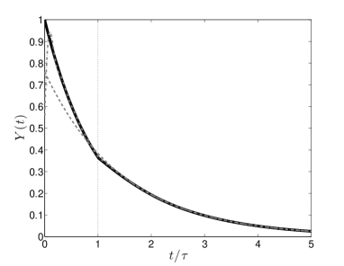
(a) $a=1$, $b=-0.16$, $\tau=1$

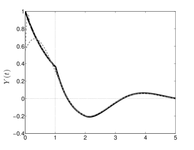
(b) $a=1$, $b=0.9$, $\tau=1$

Figure 1: The fundamental solution, $Y(t)$, plotted as a function of $t/\tau$ (solid black). Also plotted are $Y_{1}(t)$ (dashed gray) and $Y_{5}(t)$ (dashed/dotted gray) (see Eq. (15b)). In both parameter sets $\mathrm{Re\,}\lambda_{1}\simeq-0.68$.

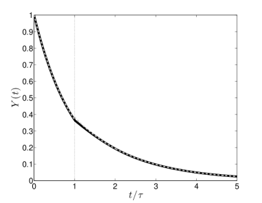
(a) $a=1$, $b=-0.16$, $\tau=1$

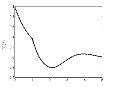
(b) $a=1$, $b=0.9$, $\tau=1$

Figure 2: Same as Fig. 1 but this time the fundamental solution is compared to expression (17). $Y_{1}(t)$ is plotted (dashed gray) for $t>\tau$ and $e^{-at}$ for $0\leq t\leq\tau$ (dashed gray).

The above can be summarized into the following expression for the fundamental solution:

$$Y(t)=\left\{\begin{array}[]{rll}&e^{-at},&\mbox{ $0\leq t\leq\tau$,}\\ \sim&Y_{1}(t),&\mbox{ $t>\tau$.}\end{array}\right.$$ (17)

The validity of expression (17) is clearly depicted in Fig. 2 where it is plotted and compared to $Y(t)$ for the two sets of parameters already shown in Fig. 1.

Notice the central difference between the fundamental solution of an ODE and a DDE. While in the former case, the behavior of the fundamental solution remains unaltered at all times, in the latter case, a distinct transition takes place at $t=\tau$. At the same time, for $t\leq\tau$, the fundamental solution of a DDE is identical to the fundamental solution of the ODE that is obtained by omitting from the DDE the terms that contain a delay time i.e. equivalent to setting $b=0$ in Eq. (6).

The reason for which so much attention is given to the fundamental solution is that the general solution to the forced delay equation (6) can be expressed in terms of it. To see this, consider the Laplace transform of Eq. (6) with initial conditions given by (7a). Provided that the forcing $f(t)$ is exponentially bounded,

$$\begin{split}h(\lambda)\,\mathcal{L}(y)(\lambda)=\phi(0)-be^{-\lambda\tau}&\int_{-\tau}^{0}e^{-\lambda\theta}\phi(\theta)\,d\theta\\ +&\int_{0}^{\infty}e^{-\lambda t}f(t)dt.\end{split}$$ (18)

Use of the convolution and inversion theorems leads to the following expression for the general solution

$$y(\phi,f)(t)=y(\phi,0)(t)+\int_{0}^{t}Y(t-t^{\prime})f(t^{\prime})\,dt^{\prime},$$ (19a)

where $$y(\phi,0)(t)$$ represents the solution to the (unforced) homogeneous delay equation (8) and is given by

$$y(\phi,0)(t)=Y(t)\phi(0)-b\int_{-\tau}^{0}Y(t-\theta-\tau)\phi(\theta)\,d\theta.$$ (19b)

Because of its similarity to ordinary differential equations, the representation of $y(\phi,f)(t)$ in this form is often referred [14] to as the variation of constants formula. Using this representation, it is easily deduced that the solution of any, either homogeneous or forced, linear delay equation is governed by its fundamental solution with the roots of the characteristic equation controlling its asymptotic behavior.

2.3 Scaling Behavior

Having presented some basic properties concerning linear DDEs, the next objective is to consider their coupling to a chaotic advection flow. For a chemical system satisfying Eq. (5), the evolution of the chemical difference between a pair of fluid parcels can be obtained by simultaneously linearizing the chemical (5) and trajectory (2a) evolution Eqs. around a fluid parcel. Using the variation of constants formula (19),

$$\begin{split}\delta C(t)=Y(t)\delta C(0)&-b\int_{-\tau}^{0}Y(t-\theta-\tau)\,\delta C(\theta)\,d\theta\\ &+\phantom{b}\int_{0}^{t}Y(t-t^{\prime})\,\left(\frac{\partial C_{0}}{\partial\bm{X}}\cdot\delta\bm{X}(t^{\prime})\right)\,dt^{\prime},\end{split}$$ (20)

where $\{\delta\bm{X}(t);\bm{X}(t)\}$, the label on the fluid parcel difference, has been suppressed for brevity. For $t\in[-\tau,0]$, $\delta C(t)=\phi(t)$ where $\phi(t)$ is a prescribed initial function.

To analyze the scaling behavior of the delay scalar field at statistical equilibrium, the long-time limit of Eq. (20) needs to be considered. A useful property for $Y(t)$ is that it is bounded with $|Y(t)|<K\exp[\mathrm{Re\,}\lambda_{1}t]$ where $K>0$ (see [14]). We impose that $a>|b|$, thus ensuring that $\mathrm{Re\,}\lambda_{1}<0$ for all $\tau>0$ (see §2.2). It follows that in the long-time limit, the first two terms that describe the evolution of the initial conditions vanish. Note that this is not the case for either marginally stable ($\mathrm{Re\,}\lambda_{1}=0$) or unstable ($\mathrm{Re\,}\lambda_{1}>0$) chemical dynamics.

At the same time, since the source depends smoothly on space, its spatial derivatives do not increase or decrease in a systematic way. Thus, the evolution of $|\delta_{\bm{X}}C_{0}(t^{\prime})|$ is closely related to the evolution of the separation between the pair of fluid parcels i.e. $\delta_{\bm{X}}C_{0}(t^{\prime})=\frac{\partial C_{0}}{\partial\bm{X}}\cdot\delta\bm{X}(t^{\prime})\sim|\delta\bm{X}(t^{\prime})|$. To obtain an expression for $|\delta\bm{X}(t^{\prime})|$ in terms of $|\delta\bm{X}(t)|$, Eq. (2a) is linearized around $\bm{X}(t^{\prime})$ from where it can be deduced that for $t>t^{\prime}$,

$$\delta\bm{X}(t^{\prime})=\bm{N}(t^{\prime},t)\delta\bm{X}(t),$$ (21a)

with

$$\bm{N}(t^{\prime},t)=\exp\left[\int_{t}^{t^{\prime}}\frac{\partial\bm{v}}{\partial\bm{X}}ds\right],$$ (21b)

where $|\delta\bm{X}(t)|$ is considered to be much less than the characteristic length scale of the velocity field, $L$, where here $L=1$. Consequently, the evolution of $|\delta\bm{X}(t^{\prime})|$ is dictated by $\bm{N}^{T}\bm{N}(t^{\prime},t)$ once calculated along the fluid parcel trajectory in backward time. Because $\bm{N}^{T}\bm{N}$ is a real, non-negative symmetric matrix, its eigenvalues are positive. Therefore, depending on its orientation at time $t$, as time $t^{\prime}$ decreases $|\delta\bm{X}(t^{\prime})|$ increases or decreases exponentially according to a set of rates whose number equals the dimension of the flow and whose values depend on the eigenvalues of $\bm{N}^{T}\bm{N}$.

In the limit of $t-t^{\prime}\rightarrow\infty$, these rates are defined as the Lyapunov exponents [31, 30]. For a two-dimensional, incompressible flow that is both ergodic and hyperbolic, all trajectories share the same set of Lyapunov exponents $\{h_{0},-h_{0}\}$ with $h_{0}>0$. It follows that for almost all orientations at time $t$, the typical separation between a pair of neighboring fluid parcels increases exponentially in backward time at a rate given by the flow Lyapunov exponent $h_{0}$ with $|\delta\bm{X}(t^{\prime})|\sim|\delta\bm{X}(t)|\exp[h_{0}(t-t^{\prime})]$.

The exponential increase of $|\delta\bm{X}(t)|$ can only be valid for the time period for which its length remains considerably less than the characteristic length scale of the velocity field. This is because for larger length scales ($\gtrsim 0.1$), linearizing the trajectory Eq. (2a) is no longer valid. For these larger length scales, finite-size effects become important and the value of $|\delta\bm{X}(t)|$ saturates at the length of the characteristic length scale of the velocity field. The time it takes for $|\delta\bm{X}(t)|$ to saturate in backward evolving time is here referred to as the stir-down time and is denoted by $T_{\delta X}$. By choosing $|\delta\bm{X}(t)|$ to be sufficiently small, an approximate expression for $T_{\delta X}$ is given by

$$T_{\delta X}=\frac{1}{h_{0}}\log(1/|\delta\bm{X}|),\quad\text{for $|\delta\bm{X}|\ll 1$}.$$ (22)

It follows that qualitatively, the evolution of a typical separation between two fluid parcels can be divided into two parts: the first one corresponding to the period that it exponentially increases and the second one to the rest of the time during which its value remains saturated. Therefore,

$$|\delta\bm{X}(t^{\prime})|\sim\begin{cases}\,|\delta\bm{X}(t)|\,e^{h_{0}(t-t^{\prime})},&\text{ for $0<t-t^{\prime}\leq T_{\delta X}$},\\ \,1,&\text{ for $t-t^{\prime}>T_{\delta X}$}.\end{cases}$$ (23)

The asymptotic behavior of the chemical difference between any two fluid parcels, and thus from (4), between any two neighboring points, may be deduced by substituting expression (23) into Eq. (20) (replacing $\bm{X}$ with $\bm{x}$ and $\delta\bm{X}$ with $\delta\bm{x}$). After making a change of variables from $t^{\prime}$ to $\Delta t=t-t^{\prime}$ and taking the limit of $t\rightarrow\infty$, the small-scale behavior ($|\delta\bm{x}\ll 1|$) is given by

$$\delta c_{\infty}(\delta\bm{x})\sim\int_{0}^{\infty}Y(\Delta t)\,\text{min}\{|\delta\bm{x}|e^{h_{0}\Delta t},1\}\,d\Delta t$$ (24)

where a number of space- and time- factors are omitted since they do not affect the scaling laws. Note that within the approximation made here, the rate of exponential increase of the separation between fluid parcels, $h_{0}$, is taken to be independent of the individual trajectories and therefore the dependence of $\delta c_{\infty}$ on $\bm{x}$ is dropped. In reality, this rate will depend on the trajectory thus modifying the average scaling behavior of the field. (See [28] for discussion of the implication of this for a linearly decaying reactive scalar. The extension of this discussion for the delay case is left for future work.)

Transition length scale

An expression equivalent to (24) was obtained by [27, 16] in the context of an ordinary reactive scalar whose reactions involve no delay time. In both cases, delay and ordinary, the asymptotic behavior of the concentration field is governed by the convolution in time of the fundamental solution associated with the chemical subsystem with the separation between fluid parcels. However, a fundamental difference between the delay reactive scalar and the ordinary reactive scalar will significantly affect the asymptotic scaling behavior of the delay scalar field and modify it with respect to the scaling behavior of the ordinary reactive scalar. This difference lies in the fundamental solution.

As discussed in §2.2, the behavior of $Y(t)$ associated with a linear DDE is distinctly different depending on whether $t/\tau$ is larger than or less than $1$. It follows that the asymptotic behavior of $\delta c_{\infty}(\delta\bm{x})$ must differ according to whether $T_{\delta x}/\tau$ is larger than or less than $1$. Since the value of $T_{\delta x}$ depends on $|\delta\bm{x}|$, this transition must occur at a certain length scale, denoted by $\delta x_{c}$, here named the transition length scale. An approximate expression for $\delta x_{c}$ may be obtained by considering the value of $|\delta\bm{x}|$ for which

$$T_{\delta x_{c}} \sim\tau,$$ (25)

from where it can be deduced that $$\delta x_{c}$$ must then approximately be equal to

$$\delta x_{c} \sim e^{-h_{0}\tau}.$$ (26)

Thus, the magnitude of the transition length scale is controlled by the product of the delay time with the flow Lyapunov exponent while it is independent of the parameter details of the reactions. Expression (26) represents the first key theoretical result of the paper.

Scaling regimes

The scaling behavior of the field is now separately examined for length scales less than and larger than the transition length scale. A good way to gain insight into this behavior is to consider the absolute value of the integrand of Eq. (24). The first function has an exponential decay (perhaps oscillatory) while the second function initially increases exponentially and then saturates. Thus the absolute value of the integrand has a distinct maximum and the dominant contribution to the integral comes from the neighborhood of this maximum. The corresponding dependence of the integral on the value of $\delta x$ implies up to three possible scaling regimes (depending on $\delta x$ and on the other parameters in the problem).

$|Y(t)\,\text{min}\{|\delta\bm{x}|e^{h_{0}t},1\}|$

(a) $T_{\delta X}>\tau$

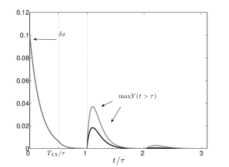
(b) $T_{\delta X}<\tau,\;|b|/ae\lesssim\delta x_{c}$

(c) $T_{\delta X}<\tau,\;|b|/(ae)\gg\delta x_{c}$

Figure 3: (a) $|Y(t)\,\text{min}\{\delta xe^{h_{0}t},1\}|$ plotted for $\delta X=10^{-4}$ ($T_{\delta X}\approx 4\tau$) for the two sets of parameters $(a,b,\tau)$ previously considered in Fig. 1: $(1,-0.16,1)$ (black) and $(1,0.9,1)$ (gray). (b) The same as (a) this time $(1,0.05,10)$ (black) and $(1,0.1,10)$ (gray) with $\delta X=10^{-1}$ so that $T_{\delta X}\approx\tau/2$. (c) The same as (b) this time $(1,0.3,10)$ (black), $(1,0.5,10)$ (dark gray) and $(1,0.75,10)$ (light gray).

Regime I   $\bm{|\delta x|<\delta x_{c}}$

The first scaling regime, Regime I, concerns length scales that are smaller than $\delta x_{c}$. For these length scales, the stir-down times are larger than the delay time and thus the chemical dynamics converge at a rate which, for the linear case considered here, is exactly given by $-\mathrm{Re\,}\lambda_{1}$ (see expressions (15b) and (17) where the ‘+’ sign is omitted since $\mathrm{Re\,}\lambda_{1}=\mathrm{Re\,}\lambda_{1}^{+}$). In analogy to the flow Lyapunov exponent that controls the strength of the flow dynamics, this rate is called the chemical Lyapunov exponent [27].

It therefore follows that within this regime, the scaling behavior of the delay reactive scalar field is no different to the scaling behavior of an ordinary reactive scalar. For both delay and ordinary scalars, the small-scale structure is controlled by the relative strength of the chemical to the flow dynamics: If $-\mathrm{Re\,}\lambda_{1}/h_{0}<1$, the chemical processes are too slow to forget the different spatial histories experienced by the fluid parcels. In this case, the maximum of $|Y(t)\,\text{min}\{|\delta\bm{x}|e^{h_{0}t},1\}|$ occurs at $t=T_{\delta x}$ (see Fig. 3(a)) and its value depends on $|\delta\bm{x}|^{-\mathrm{Re\,}\lambda_{1}/h_{0}}$. Thus, in this case, the field’s spatial structure is filamental i.e. non-differentiable in every direction except the direction along which the filaments grow [27]. On the other hand, for $-\mathrm{Re\,}\lambda_{1}/h_{0}>1$ the chemical processes converge faster to their equilibrium value than the trajectories diverge from each other. The maximum of $|Y(t)\,\text{min}\{|\delta\bm{x}|e^{h_{0}t},1\}|$ occurs at $t=0$ from where it can be deduced that the field’s structure is everywhere smooth. Thus, the Hölder exponent within Regime I is equal to $\gamma_{1}=\text{min}\{-\mathrm{Re\,}\lambda_{1}/h_{0},1\}$.

Regimes II & III  $\bm{|\delta x|>\delta x_{c}}$

Consider now length scales that are larger than $\delta x_{c}$. The corresponding stir down times are smaller than the delay time and thus the chemical dynamics converge at a rate given by $-a$, i.e. the decay rate obtained once the delay term is ignored (see expression (17)).

There exist two local maxima for $|Y(t)\,\text{min}\{|\delta\bm{x}|e^{h_{0}t},1\}|$; the first one is scale-dependent, the second one is a constant (see Figs. 3(b-c)). The value of the first local maximum is given by $\underset{t}{\text{max}}\,|e^{-at}\text{min}\,\{|\delta\bm{x}|e^{h_{0}t},1\}|=|\delta\bm{x}|^{\text{min}\{a/h_{0},1\}}$ (where $Y(t\leq\tau)=e^{-at}$ was employed (see expression (17)). It therefore follows that if this first local maximum is a global maximum, the field’s scaling behavior is described by a Hölder exponent that satisfies $\gamma_{2}=\text{min}\{a/h_{0},1\}$. This scaling regime is denoted by Regime II. Now focus on the second local maximum which is given by $\text{max}\,|Y(t\geq\tau)|$. Since this is a constant, a flat scaling regime will ensue if the second local maximum is larger than the first local maximum. This scaling regime is denoted by Regime III. However, if the second local maximum is smaller than the first local maximum, Regime III does not appear.

To investigate the range of length scales for which Regime III appears, consider in more detail $\text{max}\,|Y(t\geq\tau)|$. Now $|Y(t\geq\tau)|$ has a maximum at either $t=\tau$ or at some $t=t^{\ast}$, where $t^{\ast}$ is defined as the value of $t$ for which $dY(t)/dt$ is first equal to $0$ and thus $aY(t^{\ast})=-bY(t-t\ast)$. First consider the local maximum of $|Y(t\geq\tau)|$ to occur for $\tau<t^{\star}\leq 2\tau$. Within this time period and using the method of steps (see §2.2), $Y(t)$ can be exactly expressed as $Y(t)=e^{-at}-b(t-\tau)e^{-a(t-\tau)}$. Combining this expression with expression (11) for $Y(t)$ for $0<t\leq\tau$, $t^{\star}$ must satisfy $e^{-at^{\star}}-b(t^{\star}-\tau)e^{-a(t^{\star}-\tau)}=-b/ae^{-a(t^{\star}-\tau)}$ from where we can deduce that a local maximum of $|Y(t\geq\tau)|$ occurs if $0<1/a+1/be^{-a\tau}<\tau$. In this case, $\text{max}\,|Y(t>\tau)|=|b|/a\,e^{-1-a/be^{-a\tau}}$. Now consider $t^{\star}>2\tau$. In this case $Y(t\leq 2\tau)$ is monotonically decreasing and thus $\text{max}\,|Y(\tau\leq t\leq 2\tau)|=e^{-a\tau}$. Since $|Y(t^{\ast})|=|b|/a|Y(t-t\ast)|$, $\text{max}\,|Y(t\geq 2\tau)|\leq|b|/a\,e^{-a\tau}$ and therefore $\text{max}\,|Y(t\geq\tau)|=e^{-a\tau}$. Finally, if no $t^{\star}$ exists, then again $\text{max}|Y(t\geq\tau)|=e^{-a\tau}$. All three cases can be summarized by

$$\text{max}|Y(t\geq\tau)|=\text{max}\{e^{-a\tau},\frac{|b|}{a}e^{-1-a/be^{-a\tau}}\}.$$ (27)

Comparing the value of the first local maximum, $|\delta\bm{x}|^{\text{min}\{a/h_{0},1\}}$, with the value of the second local maximum, given by Eq. (27), we are able to obtain the following estimate for $\delta x_{2}$, the length scale that separates Regime II and III:

$$\delta x_{2}\sim\text{max}\,|Y(t\geq\tau)|^{\text{max}\{h_{0}/a,1\}}.$$ (28)

The following points can be noted:

1. If $|b|/(ae)\ll\delta x_{c}$, $\delta x_{2}\ll\delta x_{c}$ and thus there appears no Regime III.

2. If $|b|/(ae)\sim 1$, $\delta x_{2}\gg\delta x_{c}$ and thus Regime III will ensue at all length scales larger than $\delta x_{c}$.

Hölder Exponents

To summarize, the following set of scaling laws describe the spatial structure of the stationary-state delay reactive scalar field as $|\delta\bm{x}|$ varies:

$$|\delta c_{\infty}(\delta\bm{x})|\sim\begin{cases}|\delta\bm{x}|^{\gamma_{1}},&\;\text{for $|\delta\bm{x}|<\delta x_{c}$}\\ \text{flat},&\;\text{for $\delta x_{c}<|\delta\bm{x}|<\text{max}\{\delta x_{2},\delta x_{c}\}$}\\ |\delta\bm{x}|^{\gamma_{2}},&\;\text{for $|\delta\bm{x}|>\text{max}\{\delta x_{2},\delta x_{c}\}$}\end{cases}$$ (29a)

where the Hölder exponents $$\gamma_{1} \gamma_{2}$$ and are given by

$$\gamma_{1} =\text{min}\{1,-\mathrm{Re\,}\lambda_{1}/h_{0}\},$$ (29b)

$$\gamma_{2} =\text{min}\{1,a/h_{0}\}.$$ (29c)

Therefore, Regime II occurs for $|\delta\bm{x}|>\delta x_{2}$ and Regime III for $\delta x_{2}>|\delta\bm{x}|>\delta x_{c}$. It happens that Regime III will not be present if $\delta x_{2}$ and $\delta x_{c}$ are not well separated. Similarly, Regime II will not be present if $\delta x_{2}$ is not sufficiently small.

Expression (29) represents the second key theoretical result of this paper. The more general case for which several interacting chemical species are present is shown in the Appendix to be a slight variant of this expression. Special cases for which the species are not symmetrically coupled with each other may give rise to structures that are characterized by different Hölder exponents for different species. Such a case is the delay plankton model whose behavior is examined in §3.2.

3 Numerical Results: Two Examples

To complement the theoretical results obtained in the previous section, a set of numerical simulations are here performed, firstly for the single linear delay reactive scalar whose evolution within a fluid parcel was introduced in Eq. (5), and secondly for the delay plankton model that [1] first used for his numerical investigations. This model, shortly to be described, serves not only as a test-bench of the theory presented in Sec. 2 but also as an interesting application of it.

In both examples, the fluid parcels are advected by a model strain flow whose velocity field is given by

$$\bm{v}(\bm{x},t)=\left[\begin{array}[]{rl}-\displaystyle{\frac{2}{T}}\Theta(T/2-t\mod T)\cos(2\pi y+\phi)\\[5.69046pt] -\displaystyle{\frac{2}{T}}\Theta(t\mod T-T/2)\cos(2\pi x+\theta)\end{array}\right],$$ (30)

where $\Theta(t)$ is the Heaviside step function defined to be equal to unity for $t\geq 0$ and zero otherwise and $x$ and $y$ are the domain’s horizontal and vertical axis respectively. The phase angles $\theta$ and $\phi$ change randomly at each period $T$, varying the directions of expansion and contraction and hence ensuring that all parts of the flow are equally mixed [7, 30]. Variation of $T$ has an effect on the magnitude of the flow Lyapunov exponent, $h_{0}$, without changing the shape of the trajectories and the spatial structure of the flow. It may be shown that $h_{0}$ is inversely proportional to $T$ with

$$h_{0}\approx 2.33/T,$$ (31)

where the constant is numerically determined.

A large-scale inhomogeneity is injected into the system by introducing a spatially smooth forcing

$$C_{0}(\bm{x})=1-1/2\cos[2\pi(x+y)]),$$ (32)

oriented along the diagonal of the domain to avoid having the same preferred alignment to the flow. The space-dependence of the force couples the reaction dynamics with the flow dynamics and results in the formation of complex spatial patterns.

A statistical steady state is reached after approximately $20T$. To reconstruct the stationary distributions of the corresponding reactive scalars, an ensemble of fluid parcels whose final positions are fixed onto a grid are followed. Using Eq. (30), the parcels are tracked backwards in time up to a point when their initial concentrations are known. Thereafter, knowing their trajectory, their final concentration is determined by integrating the reaction equations forward in time using a second order Runge-Kutta method. This way, to obtain the concentration fields along a one-dimensional transect, it is not necessary to determine the whole two-dimensional field. The absence of interpolation permits greater accuracy at smaller length scales. The initial concentrations are chosen to be equal to their mean equilibrium values, though as long as the reaction dynamics are stable, the final result should be independent of this choice.

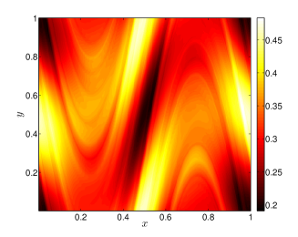
(a) $\tau=0$

(b) $\tau=1$

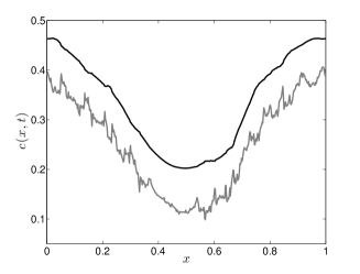
(c) Intersection

Figure 4: (Color online) Snapshots of reactive scalar distributions whose reactions evolve according to Eq. (5) at statistical equilibrium ($t=20T$). The two cases depict (a) a linearly decaying reactive scalar ($a=3$, $b=0$) for which no delay time is present and (b) a linear delay reactive scalar ($a=3$, $b=1$, $\tau=1$). The period $T=1$ such that $h_{0}\approx 2.33$ with $a>h_{0}$. The smoothly varying force is diagonally oriented given by Eq. (32). The bars on the right give the concentration values. (c) One-dimensional transects ($y=0.5$) for the linearly decaying reactive scalar (black line) and the delay reactive scalar (gray line)

The stationary distributions of a linearly decaying reactive scalar and a linear delay reactive scalar, with reactions evolving according to Eq. (5), are depicted respectively in Figs. 4(a) and (b). Notice the distinct difference between the two distributions: Fig. 4(a) contains no delay term whereas Fig. 4(b) contains a delay term and it is this delay term that is responsible for the filamental behavior of the concentration field. This difference is more easily observed in the corresponding one-dimensional transects shown in Fig. 4(c).

The most common method to characterize the scaling behavior of the distributions is to consider their Fourier power spectra. An alternative method is to consider the concentration difference between points separated by a fixed distance. The latter is called the structure function [24] and it is the method we employ here since it allows an easy comparison between the theoretical results of the previous section with the numerical results of this section. The first-order structure function associated with the field $c(\bm{x},t)$ is defined as

$$S(\delta x)\equiv\langle|\delta c(\delta\bm{x};\bm{x},t)|\rangle\sim\delta x^{\gamma},$$ (33)

where $\langle\ldots\rangle$ denotes averaging over different values of $\bm{x}$ and $\delta x\equiv|\delta\bm{x}|$. Recall that $\delta c(\delta\bm{x};\bm{x},t)\equiv\delta c(\bm{x}+\delta\bm{x},t)-\delta c(\bm{x},t)$. For the time being we assume that the $\gamma$ appearing in (33) is precisely the Hölder exponent as predicted by previous theoretical arguments.

For both the delay reactive scalar and the delay plankton model, the parameters are chosen in such a way that all three scaling regimes, described by expression (29), emerge within the range of length scales considered. To control this range, the magnitude of the characteristic length scale that separates the Regime I from Regimes II and III, denoted by $\delta x_{c}$, needs to be considered. Substituting expression (31) into (26), the expression for $\delta x_{c}$ for the model strain flow (30) becomes

$$\delta x_{c}\approx\exp(-2.33\,\tau/T).$$ (34)

Thus, the value of $\delta x_{c}$ is modified by varying the value of $\tau/T$ (see Table 3 where the value of $\delta x_{c}$ is calculated for some key values of $\tau/T$).

An estimate for the characteristic length scale, calculated for the model strain flow (30) for $L=1$ using expression (34). $\tau/T$ $1$ $2$ $3$ $4$ $\delta x_{c}$ $\approx 10^{-1}$ $\approx 10^{-2}$ $\approx 10^{-3}$ $\approx 10^{-4}$

3.1 The Linear Delay Reactive Scalar

We now examine the scaling behavior of the delay reactive scalar distribution as the value of $\tau/T$ varies. In each case, the first-order structure function is calculated over $10$ evenly spaced intersections. The scaling exponent is obtained from the slope of the first-order structure function and it is then compared to the set of scaling laws (29).

Regime I

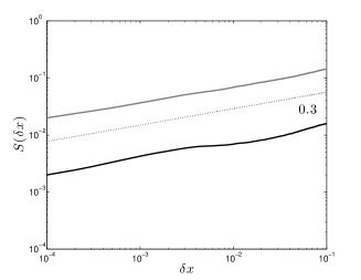
(a) $-\mathrm{Re\,}\lambda_{1}/h_{0}=0.3$

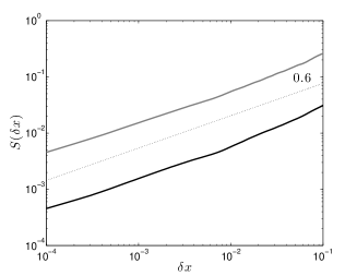
(b) $-\mathrm{Re\,}\lambda_{1}/h_{0}=0.6$

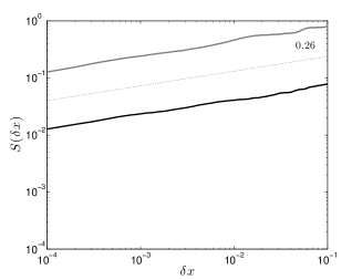
(c) $-\mathrm{Re\,}\lambda_{1}/h_{0}=0.26$

Figure 5: (a) First-order structure functions for the linear delay reactive scalar (5) averaged over $10$ evenly spaced transects (parallel to the $x$-axis). These are calculated at statistical equilibrium ($t=20T$) for the two sets of parameters $(a,b,\tau)$ that were considered in Fig. 1, both with $\mathrm{Re\,}\lambda_{1}=-0.68$ but different $\mathrm{Im\,}\lambda_{1}$: for $(1,-0.16,1)$ (gray solid line) $\lambda_{1}$ is real while for $(1,0.9,1)$ (black solid line) $\lambda_{1}$ is complex. Flow constant is $T=1$. The theoretical prediction is depicted by the dotted line. (b) Same as (a) but $T=2$. (c) Same as (a) but this time $\mathrm{Re\,}\lambda_{1}=-0.03$ with different $b$ and $\tau$ and $T$: $(1,0.92,5)$ (gray solid line), $(1,0.7,10)$ (black solid line) and $T=20$. In all cases, $\tau/T\leq 1$. Black dotted lines correspond to theoretical prediction (29b).

Regime I

Initially, $\tau/T\leq 1$ so that $\delta x_{c}\gtrsim 0.1$ (see Table 3). This way only Regime I will appear within the range of length scales considered (recall that finite-size effects become important for $\delta x>0.1$). The validity of $-\mathrm{Re\,}\lambda_{1}/h_{0}$, the ratio associated with the Hölder exponent within Regime I (see (29b)), is tested. Three different aspects are examined: the first aspect investigates the impact that the imaginary part of $\lambda_{1}$ may have on the scalar field. Recall that $\lambda_{1}$ denotes the root of the characteristic equation (9) that has the least negative real part. According to expression (29b), $\mathrm{Im\,}\lambda_{1}$ does not contribute to the field’s scaling behavior. This is confirmed in the numerical results that are shown in Fig. 5(a). There, the first-order structure functions obtained from two parameter sets, chosen so that both share the same $\mathrm{Re\,}\lambda_{1}$ but different $\mathrm{Im\,}\lambda_{1}$, are found to share the same scaling exponent (their slopes are equal). In particular, for the first set of parameters, $\lambda_{1}$ is real while for the second, $\lambda_{1}$ is complex.

The second aspect investigates how the scaling behavior varies as the value of $T$ (and therefore $h_{0}$) varies. We consider the same set of parameters as the ones in Fig. 5(a), where this time $T=2$ thus leading to a larger value for the Hölder exponent (double than before). The corresponding scaling exponents are in good agreement with the theoretical prediction (29b) (see Fig. 5(b)). Finally, the third aspect explores larger values for both $\tau$ and $T$. For two sets of parameters, both of which share the same $\mathrm{Re\,}\lambda_{1}$, the scaling exponents are in good agreement with the theoretical prediction (29b).

Regimes I & II

The coexistence of the Regimes I and II is now investigated by setting $\tau/T=2$ so that $\delta x_{c}\approx 10^{-2}$. At the same time, $\delta x_{2}\sim|b|/(ae)$ is chosen to be of the same order of magnitude as $\delta x_{c}$. This way, Regime III, whose appearance depends on the value of $\delta x_{2}$ relative to $\delta x_{c}$ (see Eq. 29) is limited. Note that because $-\mathrm{Re\,}\lambda_{1}$ increases as $|b|/a$ increases (to verify consider Eq. (9)), a smaller value of $|b|/(ae)$ results in a larger value for the Hölder exponent within Regime I. Therefore, to obtain an interesting change of behavior from Regime I to Regime II, we are limited on how small we can choose $|b|/(ae)$ to be.

To test the validity of the set of scaling laws (29), we examine the structure functions obtained from two sets of parameters, with different value for $|b|$, shown in Fig. 6(a) (see also Fig. 3(b) for comparison with theory). For the first parameter set the value of $|b|$ is smaller than for the second parameter set which implies that the first parameter set has a larger $-\mathrm{Re\,}\lambda_{1}$ than the second parameter set. Thus within Regime I, the first parameter set has a larger Hölder exponent. At the same time, $a/h_{0}>1$ for both parameter sets and thus the Hölder exponent within Regime II is equal to $1$.

Comparing the theory to the numerics, we can deduce that there is good agreement. $\delta x_{c}$ captures sufficiently well the transition between Regimes I and II. This transition occurs for slightly larger length scales for the second parameter set since it possesses a larger value of $\delta x_{2}$. Within Regime I, the field’s scaling exponent is close enough to its theoretical value, though this agreement is expected to become better for smaller length scales (see e.g. Figs. (5)). Within Regime II, the scaling exponent is, as expected, equal to $1$.

A flatter structure than predicted by theory appears for the intermediate length scales ($10^{-3}<\delta x<10^{-2}$) for which Regime I should continue to hold. It appears that this intermediate structure can be explained by noticing that the rate of exponential increase of the separation between neighboring fluid parcels is distributed. A complete development of this argument is left for future work.

Regimes I & II & III

The coexistence of the Regimes I, II and III is now investigated by keeping $\tau/T=2$ while increasing the value of $\delta x_{2}\sim|b|/(ae)$ by an order of magnitude larger than $\delta x_{c}$. This is achieved by considering the same set of parameters as in Fig. 6(a) but increasing the value of $|b|$. This increase results in an increase in the value of $\delta x_{2}$ and a decrease in the value of $-\mathrm{Re\,}\lambda_{1}$ (the value for $\delta x_{c}$ remains the same).

The structure functions corresponding to three sets of parameters, shown in Fig. 6(b) (see also Fig. 3(c) for comparison with theory), are now examined. As expected, Regime III appears within a wide range of length scales, whose range increases as the value of $|b|$ increases. The value of $\delta x_{2}$ provides a good estimate for the length scale separating Regime II from Regime III. When $|b|\sim 0.75$, $\delta x_{2}\approx 0.27$ in which case the Regime III appears for all length scales larger than $\delta x_{c}$, thus displacing Regime II (see Fig. 6(b)). Similarly to the numerical results shown in Fig. 6(a), a good agreement between theory and numerics is obtained within Regime I, the agreement being better for smaller length scales (the flat regime also appearing here). As before, the field’s scaling behavior within Regime II is smooth.

Regimes I & II

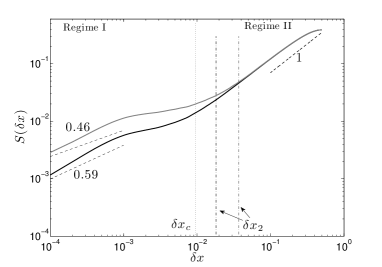
(a) $|b|/(ae)\sim\delta x_{c}$

Regimes I & II & III

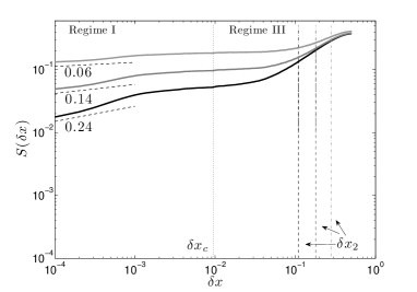
(b) $|b|/(ae)\gg\delta x_{c}$

Figure 6: Same as Fig. 5 but this time $\delta x_{c}\approx 0.01$ ($\tau/T=2$). The set of parameters $(a,b,\tau)$ are: (a) $(1,0.05,10)$ (black) with $\delta x_{2}\approx 0.02$ and $(1,0.1,10)$ (black) with $\delta x_{2}\approx 0.04$. (b) $(1,0.3,10)$ (black) with $\delta x_{2}\approx 0.11$ , $(1,0.5,10)$ (dark gray) with $\delta x_{2}\approx 0.18$ and $(1,0.75,10)$ (light gray) $\delta x_{2}\approx 0.27$. In all cases $T=5$ which leads to $a>h_{0}$. Also shown are the predictions for the Hölder exponents (black dashed lines), $\delta x_{c}$ (black dotted line) and $\delta x_{2}$, based on the estimate given by (28) (dashed-dotted line with different shades for each parameter set).

3.2 The Delay Plankton Model

Having investigated the scaling behavior of the linear delay reactive scalar field, the focus now turns to the delay plankton model. This is a typical nutrient-predator-prey system [25] where the effect of the former is parameterised by the prey carrying capacity, denoted by $C$. The interactions among the biological species are given by the following set of nonlinear delay-differential equations

$$\frac{dC}{dt} =\alpha(C_{0}(\bm{x})-C),$$ (35a)

$$\frac{dP}{dt} =P(1-P/C)-PZ,$$ (35b)

$$\frac{dZ}{dt} =P(t-\tau)Z(t-\tau)-\delta Z^{2},$$ (35c)

where $P$ stands for phytoplankton and $Z$ for zooplankton, $t$ is a dimensionless time scaled to the phytoplankton production rate $r$ ($t/r$ is the real time) and $\alpha$ denotes the rate at which the carrying capacity relaxes to the background source $C_{0}(\bm{x})$. The phytoplankton growth is logistic and grazing takes place according to a simple $PZ$ term. Zooplankton death occurs at a rate $\delta$ and is described by a quadratic in $Z$ term, representing grazing due to higher trophic levels. The key feature of this model is the introduction of the time $\tau$ that represents the time it takes for the zooplankton to mature ($\tau/r$ in real time). For although it is reasonable to assume an instantaneous change in the prey population once prey and predator are encountered, it is not reasonable to assume an instantaneous change in the predator population.

The stationary distributions for $C$, $P$ and $Z$, attained when coupled to the strain model flow (30), are depicted for a particular set of parameters in Fig. 7. Before analyzing any numerical simulations, the particular plankton dynamics need first to be examined. While the scaling behavior of a general system of delay reactive scalar fields has been set out in the Appendix, certain non-generic features are easier to address for each model in question.

For the delay plankton model, the non-generic feature is the existence of asymmetrical couplings between the phytoplankton’s carrying capacity and the subsystem comprising of the phytoplankton and the zooplankton. [16] considered the case of a zero delay time and deduced that the phytoplankton and zooplankton should always share the same small-scale structure. The numerical results that [36] obtained show that the same holds for a non-zero delay time, provided the length scales remain sufficiently small. However, on larger scales, a second scaling regime appears in which the zooplankton structure is flat while the phytoplankton has a structure similar to its carrying capacity. Although the appearance of a second scaling regime is inherent to any system of delay reactive scalar fields, the decoupling among the species is particular to the delay plankton model.

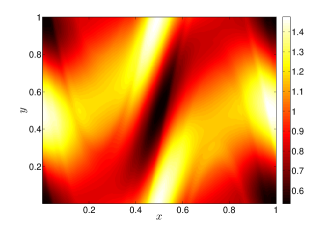
(a) Carrying Capacity

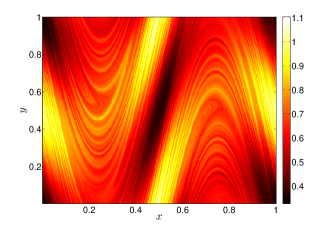
(b) Phytoplankton

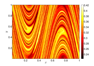
(c) Zooplankton

Figure 7: (Color online) Snapshots of the biological distributions at statistical equilibrium ($t=20T$) for the delay plankton model (35) stirred by the model strain flow (30) with $\tau=20$, $\alpha=0.25$, $\delta=2$ and $T=20$. As before the force is diagonally oriented, described by (32).

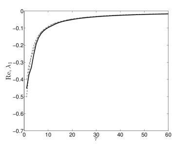
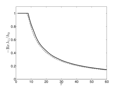
Figure 8: (a) The value of $\mathrm{Re\,}\lambda_{1}$, associated with the rate of the slowest decaying eigenfunction of the linearized phytoplankton-zooplankton subsystem, calculated and plotted as a function of $\tau$ for $C_{0}=1$ (black solid line), $C_{0}=0.5$ (gray dashed line) and $C_{0}=1.5$ (gray dashed-dotted line) ($\delta=2$). Its value is determined by considering the roots of the characteristic Eq. (39). (b) The value of $\text{min}\{-\mathrm{Re\,}\lambda_{1}/h_{0},1\}$, the theoretical value for the Hölder exponent shared between the phytoplankton and the zooplankton, plotted as a function of $\tau$ for $h_{0}\approx 0.117$ ($T=20$) and $C_{0}=1$ (black solid line), $C_{0}=0.5$ (gray dashed line) and $C_{0}=1.5$ (gray dashed-dotted line).

To fully explain the scaling behavior of the delay plankton model, the theory of Sec. 2 must be extended in order to accommodate the particularities of this model. In the absence of advection and within a certain range of parameters, the delay plankton model has a single fixed point of equilibrium, given by

$$C^{\star}=C_{0}(\bm{x}),\;P^{\star}=\delta C^{\star}/(\delta+C^{\star})\;\text{and}\;Z^{\star}=P^{\star}/\delta.$$ (36)

This point is stable for $\tau=0$. For $0.5\leq C_{0}(\bm{x})\leq 1.5$ and $\delta=2$, as in the simulations performed here, this point remains stable for any $\tau>0$. Linearizing the delay plankton model around this point of equilibrium results in the following expressions for the matrices $\bm{A}$ and $\bm{B}$:

$$\bm{A}=\left(\begin{matrix}\alpha&0&0\\ -(P^{\ast}/C^{\ast})^{2}&P^{\ast}/C^{\ast}&P^{\ast}\\ 0&0&2P^{\ast}\end{matrix}\right)$$ (37a)

and

$$\bm{B}=-P^{\ast}\left(\begin{matrix}0&0&0\\ 0&0&0\\ 0&1/\delta&1\end{matrix}\right)$$ , (37b)

where $\bm{A}$ and $\bm{B}$ are the matricial equivalents of $a$ and $b$ for the one-dimensional linear delay reactive scalar (5) (for further details see App. (A)). Certain matrix coefficients (i.e. $-(P^{\ast}/C^{\ast})^{2}$, $P^{\ast}/C^{\ast}$, $2P^{\ast}$) were simplified using (36).

From Eq. (A3), the characteristic matrix is given by $\bm{H}(\lambda)=\lambda\bm{I}+\bm{A}+\bm{B}e^{-\lambda\tau}$. Thus, using Eq. (37),

$$\begin{split}&\bm{H}(\lambda)=\\ &\left(\begin{matrix}\lambda+\alpha&0&0\\ -\left(P^{\ast}/C^{\ast}\right)^{2}&\lambda+P^{\ast}/C^{\ast}&P^{\ast}\\ 0&-e^{-\lambda\tau}P^{\ast}/\delta&\lambda-P^{\ast}e^{-\lambda\tau}+2P^{\ast}\end{matrix}\right).\end{split}$$ (38)

It follows that the characteristic equation corresponding to the linearized delay plankton model satisfies (see Eq. (A3))

$$h(\lambda)\equiv\text{det}\bm{H}(\lambda)=(\lambda+\alpha)\,g(\lambda)=0,$$ (39a)

where $$g(\lambda)=0$$ is the characteristic equation associated with the phytoplankton-zooplankton subsystem.

$$g(\lambda)=\left|\begin{matrix}\lambda+P^{\ast}/C^{\ast}&P^{\ast}\\ -e^{-\lambda\tau}P^{\ast}/\delta&\lambda-P^{\ast}e^{-\lambda\tau}+2P^{\ast}\end{matrix}\right|.$$ (39b)

As in the one-dimensional case, the number of roots are infinite for $g(\lambda)=0$ (and therefore for $h(\lambda)=0$). At the same time, the magnitude of $\mathrm{Re\,}\lambda_{1}$, the root with the least negative real part, decreases as $\tau$ increases with $\mathrm{Re\,}\lambda_{1}\rightarrow 0$ as $\tau\rightarrow\infty$. Its value is determined for fixed $C_{0}$ and $\delta$ and plotted in Fig. 8(a) as a function of $\tau$ for $\delta=2$ and three key values of $C_{0}(\bm{x})$: $1$, $1.5$ and $0.5$ i.e. its average, maximum and minimum (see Eq. (32)). Notice that the difference between the $\mathrm{Re\,}\lambda_{1}$ calculated for these three values of $C_{0}(\bm{x})$ is minor. It is therefore expected that the value for the least negative chemical Lyapunov exponent associated with the nonlinear dynamics of the delay plankton model is close to $-\mathrm{Re\,}\lambda_{1}$.

In the theoretical considerations made in Sec. 2, the scaling behavior of a linear delay reactive scalar was described by the set of scaling laws (29). A similar set of scaling laws holds for a system of nonlinearly interacting scalars (see App. B): the Hölder exponent within Regime I is governed by the ratio of the least negative chemical Lyapunov exponent, -$\mathrm{Re\,}\lambda_{1}$, to the flow Lyapunov exponent, $h_{0}$; within Regime II, the Hölder exponent is governed by $-a_{1}/h_{0}$, where $a_{1}$ is the slowest decay rate associated with the reduced system that is obtained once all delay terms are ignored. As for the single delay reactive scalar, the appearance of a flat scaling regime, Regime III, depends on whether $\delta x_{2}$, the length scale associated with this regime, is larger than $\delta x_{c}$, the transition lengthscale. Note that the value of $\delta x_{2}$ is not necessarily the same for each species (see §B).

This set of scaling laws was deduced for the general case in which the product of the fundamental matrix, the matricial equivalent of the fundamental solution (see §A), with the direction of the forcing in the chemical space has non-zero entries (see Eq. (20)). If that is not the case, the set of scaling laws (29) may need to be modified and different regimes for different species are expected. Note however that in all cases the value of $\delta x_{c}$ is not affected as its value only depends on $\tau$ and not on the particular chemical dynamics.

To examine the existence of zero entries for the linearized delay plankton model, consider first the form of the eigenfunctions that comprise its fundamental matrix. This matrix, denoted by $\bm{M}_{\bm{Y}}(t)$, can be written as an infinite sum of eigenfunctions, each proportional to $e^{\lambda_{i}t}\text{adj}\bm{H}(\lambda_{i})$, where adj is short for adjoint (see Eq. (A7)). In the delay plankton model, the forcing is given by the source $C_{0}(\bm{x})$. Since this is applied only to the carrying capacity, the product of $\text{adj}\bm{H}(\lambda_{i})$ with the forcing direction is given by

$$\text{adj}\bm{H}(\lambda_{i})\cdot\left(\begin{matrix}1\\ 0\\ 0\end{matrix}\right)=\left(\begin{matrix}\phantom{m}g(\lambda_{i})\\ m_{1}(\lambda_{i})\\ m_{2}(\lambda_{i})\end{matrix}\right)$$ (40)

with

$$m_{1}(\lambda_{i}) =(\lambda_{i}-P^{\ast}[e^{-\lambda_{i}\tau}-2])(P^{\ast}/C^{\ast})^{2},$$ (41a)

$$m_{2}(\lambda_{i}) =e^{-\lambda_{i}\tau}{P^{\ast}}^{3}(\delta C^{\ast})^{-1},$$ (41b)

where to deduce the above, Eqs. (38) and (39) were employed.

Examining the behavior of Eq. (40) as a function of $\lambda_{i}$ where $h(\lambda_{i})=0$ and $i=1\ldots\infty$, it can be deduced that as long as these are distinct (achieved by appropriately choosing the parameter range), the only $\lambda_{i}$ for which $g(\lambda_{i})\neq 0$ is $\lambda_{i}=-\alpha$. Therefore, a single eigenfunction governs the scaling behavior of $C$ from where it can be inferred that a single Hölder exponent characterizes its spatial structure. Its value is given by

$$\gamma_{C}=\text{min}\{1,\alpha/h_{0}\}.$$ (42)

This result is hardly surprising as it is easy to observe that the carrying capacity evolves independent of the rest of the species and as the much studied linearly decaying scalar with chemical Lyapunov exponent equal to $-\alpha$.

On the other hand $m_{1}(\lambda_{i})$, $m_{2}(\lambda_{i})\neq 0$ for all $\lambda_{i}$, where $i=1\ldots\infty$ and thus no special considerations are necessary for the phytoplankton and zooplankton; their scaling behavior within Regime I is shared and governed by the least negative chemical Lyapunov exponent, $\mathrm{Re\,}\lambda_{1}$.

However, within Regime II a different scenario takes place. The fundamental matrix corresponding to this regime may be exactly written as $\bm{M}_{\bm{Y}}(t)=\exp[-\bm{A}t]$ (see App. A). Using a singular value decomposition, $\bm{M}_{\bm{Y}}(t)$ can be re-written in terms of $\bm{\hat{a}}_{i}e^{a_{i}t}\bm{\hat{a}}_{i}^{{\dagger}}$ where $\bm{\hat{a}}_{i}$ and $\bm{\hat{a}}_{i}^{{\dagger}}$ correspond to the normalized right and left eigenvectors of $\bm{A}$ with eigenvalue $a_{i}$ where $i=1\ldots 3$. To understand the scaling behavior of the phytoplankton and zooplankton, it is necessary to consider for each $i$, the product of $\bm{\hat{a}}_{i}e^{a_{i}t}\bm{\hat{a}}_{i}^{{\dagger}}$ with the forcing direction. The eigenvalues of $\bm{A}$ are given by

$$\{a_{1},a_{2},a_{3}\} =\{-\alpha,-P^{\ast}/C^{\ast},-2P^{\ast}\},$$ (43a)

while the product of $$\bm{\hat{a}}_{i}e^{a_{i}t}\bm{\hat{a}}_{i}^{{\dagger}}$$ with the forcing direction is given by

$$\left\{\bm{\hat{a}}_{i}e^{-a_{i}t}\bm{\hat{a}}_{i}^{{\dagger}}\cdot\left(\begin{matrix}1\\ 0\\ 0\end{matrix}\right)\right\} =\left\{e^{-\alpha t}\left(\begin{matrix}\cdot\\ \cdot\\ 0\end{matrix}\right),e^{-P^{\ast}/C^{\ast}t}\left(\begin{matrix}0\\ \cdot\\ \cdot\end{matrix}\right),e^{-2P^{\ast}t}\left(\begin{matrix}0\\ 0\\ 0\end{matrix}\right)\right\}.$$ (43b)

where $(\cdot)$ indicates that the dependence on (non-zero) constants has been suppressed for brevity as their magnitude does not increase or decrease in a systematic way and therefore they do not contribute to the fields’ scaling laws (see §B).

It follows that, within Regime II, two terms that are decaying exponentially with rates $-\alpha$ and $-\lambda_{P}=-P^{\ast}/C^{\ast}$ contribute to the scaling behavior of the phytoplankton. The term that corresponds to the smallest decay rate will dominate the scaling behavior of the phytoplankton (see also App. B). Note that in all the simulations performed here, $\alpha<P^{\ast}/C^{\ast}$ where the value of $P^{\ast}/C^{\ast}$ is calculated for $0.5\leq C_{0}(\bm{x})\leq 1.5$, the range of values of $C_{0}(\bm{x})$ (see Eqs. (32) and (36)). It is therefore expected that the scaling behavior of the phytoplankton is dominated by $-\alpha$, the same rate that determines its carrying capacity. Conversely, none of these terms contribute to the scaling behavior of the zooplankton, implying that within Regime II, the zooplankton is decoupled from the biological forcing and thus evolves like a passive tracer. Therefore, within this regime, its spatial structure is flat.

As a consequence Regime III appears in the scaling behavior of the phytoplankton only. The value for $\delta x_{2}$ separating Regimes II and III maybe estimated using Eq. (A22). In all numerical simulations performed here, $\delta x_{2}\lesssim\delta x_{c}$ and therefore this flat regime is not prevalent in the scaling behavior of the phytoplankton.

The following set of expressions for the Hölder exponents associated with the phytoplankton, $\gamma_{P}$, and the zooplankton, $\gamma_{Z}$, describe the distributions scaling behavior within the two regimes:

• For Regime I,

  $$\phantom{X}\gamma_{PZ}=\gamma_{P}=\gamma_{Z}=\text{min}\{\gamma_{C},-\mathrm{Re\,}\lambda_{1}/h_{0}\}.$$ (44a)

• For Regime II,

  $$\begin{split}\quad\gamma_{P}\neq\gamma_{Z}\;\text{with}\;&\gamma_{P}=\text{min}\{\gamma_{C},-\lambda_{P}/h_{0}\},\\ &\gamma_{Z}=0.\end{split}$$ (44b)

To summarize, within Regime I, $P$ and $Z$ share the same small-scale structure characterized by the Hölder exponent $\gamma_{PZ}$. This structure is either shared by $C$ i.e. $\gamma_{PZ}=\gamma_{C}$ (see Eq. (42) for $\gamma_{C}$), or is more filamental than $C$ i.e. $\gamma_{PZ}<\gamma_{C}$. Within Regime II, the small-scale structure of $Z$ is flat (zero Hölder exponent) while that of $P$ is either shared with $C$ or is more filamental than $C$.

The numerical results obtained from a set of simulations performed firstly for a varying value of $\tau$, and secondly for a varying value of $T$ are now analyzed.

Varying $\tau$

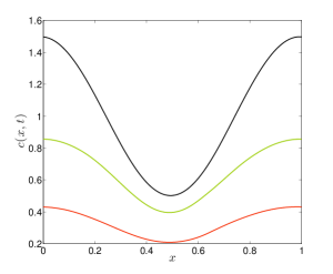
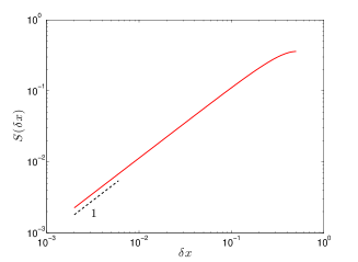
(a) $\tau=1$

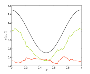
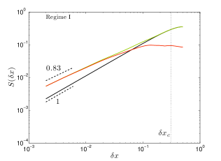
(b) $\tau=10$

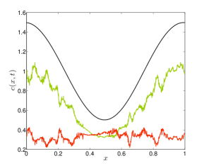
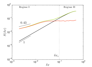
(c) $\tau=20$

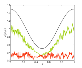
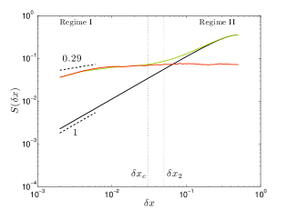
(d) $\tau=30$

Figure 9: (Color online) Representative intersections ($y=0.5$) (left) and their corresponding first-order structure functions averaged over 500 evenly spaced intersections (right) at statistical equilibrium ($t=20T$) for the delay plankton model (35) advected by (30) for $\delta=2$, $T=20$ and $\alpha=0.25>h_{0}\approx 0.117$. Graphs show carrying capacity in black, phytoplankton in light gray (green) and zooplankton in dark gray (red). The value of $\delta x_{c}$ is marked by a vertical dotted black line (if $\delta x_{c}<0.5$) and the value of $\delta x_{2}$ is marked if it is larger than $\delta x_{c}$. A dotted line for each slope of gradient equal to the theoretical value of the Hölder exponent is drawn for reference.

Variation of $\bm{\tau}$

In the set of numerical results shown in Fig. 9, the evolution of the concentration fields (calculated over an intersection) and their first-order structure functions (calculated over $500$ evenly spaced horizontal intersections) corresponding to the zooplankton, phytoplankton and its carrying capacity, are examined as a function of $\tau$. Note that the structure functions have been offset to emphasise that for small $\tau$ all species share the same behavior at all length scales. For larger $\tau$, the phytoplankton and zooplankton share the same structure at small length scales while at larger length scales the phytoplankton shares the same structure as its carrying capacity.

Starting from a small value for $\tau$ for which only Regime I appears and in which all the planktonic distributions are smooth (Fig. 9(a)), the behavior of both the phytoplankton and the zooplankton becomes increasingly filamental as the value of $\tau$ increases (Fig. 9(b-d)). This behavior is in agreement with the prediction that the magnitude of their shared chemical Lyapunov exponent decreases as $\tau$ increases, approaching zero for large values of $\tau$ (see Fig.8(a)). A comparison between theory and numerics within Regime I may be made by consulting Fig. 8(b) where the Hölder exponent, given by $\text{min}\{-\mathrm{Re\,}\lambda_{1}/h_{0},1\}$, is calculated and plotted as a function of $\tau$ for the same values of $C_{0}(\bm{x})$ as in Fig. 8(a). As a reference, a line of the same slope as the theoretical value for the Hölder exponent is drawn for each case depicted in Fig. 9(a-d). The agreement between theory and numerics is very close.

At the same time as the value of $\tau$ increases, the value of the transition length scale decreases according to the theoretical expression (34). This leads to the appearance of Regime II. Within the latter regime, the theoretical prediction is confirmed: the distribution of the phytoplankton is smooth and similar to the distribution of its carrying capacity while that of the zooplankton is flat, equivalent to the distribution of a passive (non-reactive) tracer. The theoretical value for $\delta x_{c}$ predicts sufficiently well the transition between the first and second scaling regime.

For Figs. 9(a-c)), $\delta x_{2}<\delta x_{c}$, thus explaining why no Regime III is observed for the phytoplankton (where to estimate $\delta x_{2}$, Eq. (A22) was used). The only exception is shown in Fig. 9(d) for which $\tau=30$. For this case $\delta x_{2}\sim\delta x_{c}$ and thus within a short region of length scales, a flat regime is predicted to appear for the phytoplankton. Indeed a flat regime is observed but as in the case of the single delay scalar (see §3.1), this flat regime is extended to length scales that lie within Regime I (though still close to $\delta x_{c}$). A larger value of $\delta x_{2}$ is obtained by further increasing the value of $\tau$. This is clearly depicted in Fig. 10(a) where Regime III appears for a substantial range of length scales. For scales larger than $\delta x_{2}$, Regime II appears.

Variation of $\bm{T}$

The evolution of the concentration fields and their first-order structure functions, are now examined as a function of the stirring strength of the flow, the latter parameterised by the value of $T$, and shown in Fig. (10). Starting from Fig. (10(a)), as the value of $T$ increases, so does the value for $\delta x_{c}$ (see Eq. (34)) along with the range of length scales for which Regime I appears. Again, the agreement between theory and numerics is close with $\delta x_{c}$ providing a good prediction for when the transition from Regime I to either Regime III (see Fig. 10(a)) or Regime II (see Figs. 10(b-c)) occurs.

Varying $T$

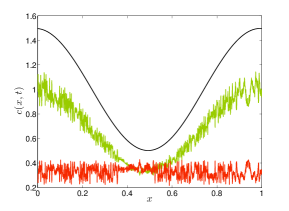
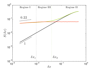
(a) $T=20$

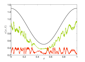
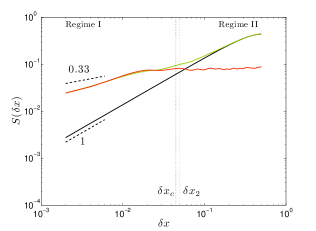
(b) $T=30$

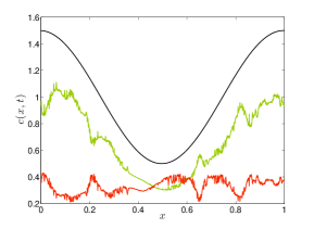
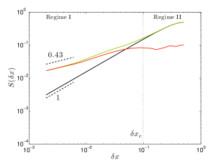
(c) $T=40$

Figure 10: (Color online) Same as Fig. 9 but this time the flow parameter $T$ varies ($\tau=40$, $\delta=2$).

4 Summary and Conclusions

This paper has considered the spatial properties of chaotically advected delay reactive scalar fields, i.e. scalar fields whose reactions explicitly contain a delay time. The investigation was motivated by the need for a theoretical explanation for previous numerical results obtained for a delay plankton model [1, 36] but the results are relevant to other chemical and biological systems [32, 25].

The system considered had stable reaction dynamics in which spatial inhomogeneity is forced by a spatially smooth source and in which the reacting species are advected by a two-dimensional, unsteady and incompressible flow. The case of reactions described by a single linear delay equation was considered in detail as a simple prototype and the results were then extended to a reaction described by a system of nonlinearly interacting delay equations. Two main conclusions were drawn concerning the scaling behavior of the delay reactive scalar fields. The first was that, no matter how large the value of the delay time, at sufficiently small length scales the scaling behavior is characterized by a Hölder exponent whose value depends on the ratio of the slowest decay rate associated with the reaction dynamics, i.e. the least negative chemical Lyapunov exponent, to the flow Lyapunov exponent. Thus, within this scaling regime, denoted as Regime I, the introduction of a delay time into the reactions results in a scaling behavior that is a straightforward generalization of that for which there is no delay time. For the particular case of the delay plankton model, this implies that the phytoplankton and zooplankton share the same scaling behavior at small scales.

On the other hand, when the stirring of the flow is sufficiently strong or the delay time is sufficiently large, the scaling behavior undergoes a change beyond a transition lengthscale. The expression for the transition length scale was deduced to depend on both the stirring strength and the delay time, exponentially decreasing as a function of their product. This change of behavior is inherent to the delay system and may be described by three different scenarios: The first scenario occurs when a second scaling regime, denoted as Regime II, is created to accompany the first scaling regime. This new scaling regime appears at all small-scales that are larger than the transition length scale. The scaling behavior within this second regime is essentially captured by a reduced reaction system in which all reaction terms that contain a delay time are ignored. The value of the corresponding Hölder exponent depends on the ratio of the slowest decay rate associated with the reduced reactive processes to the flow Lyapunov exponent. For the particular case of the delay plankton model, this result explains why the zooplankton assumes a similar distribution to a passive (non-reactive) scalar while the phytoplankton assumes a different less-filamental distribution. A second scenario occurs when the second scaling regime is preceded by a flat scaling regime, denoted as Regime III. In this case there are three scaling regimes present: Regimes I, II and III. For this to happen, the transition length scale needs to be small compared to the ratio of the reaction terms that contain a delay time to those terms that do not. As this ratio increases, so does the range of length scales for which Regime III appears. When this ratio reaches the order of unity, a last scenario occurs in which the Regime III appears at all small-scales that are larger than the transition length scale. In this case Regime II does not appear.

We believe that the investigation presented here resolves the main issues concerning the small-scale spatial structure of chaotically advected delay reactive scalar fields. Although the models under consideration are highly simplified, they can be readily extended to include any number of interacting species or space-dependent productivity and death rates. As long as the reactions are stable, the above conclusions remain unchanged.

There are, however, details that need further examination. This paper has avoided the implications of a distribution of finite-time flow and chemical Lyapunov exponents. Some of the implications of a distribution of finite-time flow Lyapunov exponents have been addressed by [28]. The implications of a distribution of finite-time chemical Lyapunov exponents, avoided in this paper by basing discussion on solutions of model chemical systems with constant coefficients, could be incorporated in a similar way. It is believed that including these effects may give a better description of the fields’ scaling behavior within Regime I for length scales close to the transition length scale.

The primary theoretical predictions of this paper are the parameter dependence of the scaling behavior in three different regimes and the transition length scales between those regimes. This makes it possible to develop a quantitative evaluation of the theory, for example, as applied to observations of ocean plankton distributions at the mesoscale; one of the principal motivations for the line of investigation in this paper. Depending on the time it takes for the zooplankton to mature and the stirring induced by the straining activity of the mesoscale eddies, three, instead of one, scaling regimes may characterize the plankton distributions. Given the differing spatial distributions exhibited by the plankton at the open mesoscale ocean [19, 34, 23], it is worth taking into account the existence of these two new scaling regimes when trying to interpret oceanic measurements at a large range of length scales. A degree of care should be taken however as the ocean is highly complex and the presence of small-scale forcing is ubiquitous in the ocean, reflecting not only the individual zooplankton behavior but also the presence of strong localized upwelling. Because the impact that these processes have on larger scales may be significant [21, 22], it is important to build the complexity of the idealised models considered here by including both more realistic dynamics, in which vertical effects and frontal circulation are taken into account, as well as some of the characteristics of the individual zooplankton behavior such as diurnal vertical migration. Finally, the distinct role that a delay time plays on the formation of structures in reactive scalar distributions is expected to prompt further research on the subject. But it should be emphasized the results presented in this paper have potential application beyond the field of ocean sciences, to any system involving fluid flow and chemical or biological interactions.

Acknowledgments. The authors are grateful to B. Legras, J. H. P. Dawes and A. P. Martin for their useful comments as well as A. Iserles for his insight. AT is currently supported by the Marie Curie Individual fellowship HydraMitra No. 221827.

Appendix: System of Delay Reactive Scalars

In this appendix we extend the theoretical results obtained in Sec. 2 for a single delay reactive scalar to a system of such fields.

A Key Properties of a System of Forced Linear Delay Equations

Consider a system of forced, linear DDEs,

$$\dot{\bm{y}}=-\bm{A}\,\bm{y}(t)-\bm{B}\,\bm{y}(t-\tau)+\bm{f}(t),$$ (A1)

where $\bm{A}$, $\bm{B}$ $\in\mathbb{R}^{n\times n}$ and $\bm{y}$, $\bm{f}$ $\in\mathbb{R}^{n}$. Retracing the same steps as for the single case (6), the characteristic equation that corresponds to the homogeneous part of Eq. (A1),

$$\dot{\bm{y}}=-\bm{A}\,\bm{y}(t)-\bm{B}\,\bm{y}(t-\tau),$$ (A2)

is obtained by looking for solutions of the form $\bm{c}e^{\lambda t}$, where $\bm{c}\in\mathbb{R}^{n}$, and $\lambda\in\mathbb{C}$. The form of the characteristic equation is given by

$$h(\lambda)\equiv\text{det}\bm{H}(\lambda)\equiv|\lambda\bm{I}+\bm{A}+\bm{B}e^{-\lambda\tau}|=0,$$ (A3)

where $\bm{H}(\lambda)$ is defined as the characteristic matrix.

The fundamental matrix, is defined as the matricial solution to (A2) with initial conditions

$$\bm{M}_{\bm{Y}}(t)=\left\{\begin{array}[]{rl}\bm{0},&\mbox{ $t<0$,}\\ \bm{I},&\mbox{ $t=0$.}\end{array}\right.$$ (A4)

For $0\leq t\leq\tau$, an exact expression for $\bm{M}_{\bm{Y}}(t)$ can be obtained using the method of steps (see §2.2). For $t>\tau$ it is more useful to take the Laplace transform of $\bm{M}_{\bm{Y}}(t)$. Using Eq. (A2),

$$\mathcal{L}(\bm{Y})(\lambda)=\bm{H}^{-1}(\lambda)\cdot\bm{1}.$$ (A5)

from where

$$\bm{M}_{\bm{Y}}(t)=\int_{(\gamma)}e^{\lambda t}\bm{H}^{-1}(\lambda)\,d\lambda,\quad t>0,$$ (A6)

where $\gamma>\text{max}\{\mathrm{Re\,}\lambda:h(\lambda)=0\}$. The inverse of $\bm{H}(\lambda)$ can be written in terms of its matrix of cofactors, $\text{adj}\bm{H}(\lambda)$, and its determinant $h(\lambda)$. Integrating $e^{\lambda t}\bm{H}^{-1}(\lambda)$ along a suitably chosen contour results in

$$\bm{M}_{\bm{Y}}(t)=\sum_{j=0}^{\infty}\underset{\lambda=\lambda_{j}}{\text{Res}}e^{\lambda t}\frac{\text{adj}\bm{H}(\lambda)}{h(\lambda)},\quad t>0,$$ (A7)

where, similarly to the single case, the infinite series (A7) is proved [37] to be uniformly convergent in $t$. Because $\bm{A},\bm{B}$ are real, the roots of (A3) are either real or come in complex conjugate pairs. For parameters chosen so that all roots are distinct, $e^{\lambda t}\bm{H}^{-1}(\lambda)$ only has simple poles. By combining the contributions from each complex conjugate pair, (A7) becomes

$$\bm{M}_{\bm{Y}}(t)=\lim\limits_{N\rightarrow\infty}\bm{M}_{\bm{Y}_{N}}(t),\quad t>0,$$ (A8a)

where $$\bm{M}_{\bm{Y}_{N}}(t)$$ is equal to

$$\bm{M}_{\bm{Y}_{N}}(t)=\sum_{\begin{subarray}{c}j=1\\ \{\lambda_{j}^{+}:\,\mathrm{Im\,}\lambda_{j}\geq 0\}\end{subarray}}^{N}e^{\mathrm{Re\,}\lambda_{j}^{+}t}\bm{\hat{H}}(\lambda_{j}^{+},t)$$ (A8b)

with $$\mathrm{Re\,}\lambda_{j}^{+}>\mathrm{Re\,}\lambda_{j+1}^{+} \bm{\hat{H}}(\lambda_{j}^{+},t)$$. is a real matrix equal to

$$\bm{\hat{H}}(\lambda_{j}^{+},t)=2^{\mathcal{H}(\mathrm{Im\,}\lambda_{j}^{+})}\,\mathrm{Re\,}\left(e^{i\mathrm{Im\,}\lambda_{j}^{+}t}\frac{\text{adj}\bm{H}(\lambda_{j}^{+})}{h^{\prime}(\lambda_{j}^{+})}\right),$$ (A8c)

with $\mathcal{H}(x)$ previously defined in Eq. (15e). Hence, for sufficiently large $t$, the behavior of $\bm{M}_{\bm{Y}_{N}}(t)$ is dominated by $\bm{M}_{\bm{Y}_{1}}(t)$. Therefore, $\bm{M}_{\bm{Y}_{N}}(t)$ satisfies the following approximate expression

$$\bm{M}_{\bm{Y}}(t)=\left\{\begin{array}[]{rll}&e^{-\bm{A}t},&\mbox{ $0\leq t\leq\tau$,}\\ \sim&\bm{M}_{\bm{Y}_{1}}(t),&\mbox{ $t>\tau$.}\end{array}\right.$$ (A9)

Thus, similarly to the fundamental solution corresponding to a single DDE (see Eq. (17)), the behavior of the fundamental matrix of a system of linear DDEs is distinctly different to the behavior of the fundamental matrix of a system of linear ODEs. At the same time, for $t\leq\tau$, the fundamental matrix obtained by setting $\bm{B}=\bm{0}$ in Eq. (6) is identical to $\bm{M}_{\bm{Y}}(t)$.

The general solution to Eq. (A1) depends on $\bm{M}_{\bm{Y}}(t)$. Let this solution be denoted by $\bm{y}(\bm{\phi},\bm{f})(t)$, where $\bm{\phi}(t)$ represents the initial conditions given by

$$\bm{y}(t)=\bm{\phi}(t),\quad t\in[-\tau,0].$$ (A10)

Provided that the forcing, $\bm{f}(t)$, is exponentially bounded, $\bm{y}(\bm{\phi},\bm{f})(t)$, is obtained by considering the Laplace transform of Eq. (A1). This leads to

$$\begin{split}\bm{H}(\lambda)\mathcal{L}(\bm{y})(\lambda)=\bm{\phi}(0)-e^{-\lambda\tau}\bm{B}\cdot&\int_{-\tau}^{0}e^{-\lambda\theta}\bm{\phi}(\theta)d\theta\\ +&\int_{0}^{\infty}e^{-\lambda t}\bm{f}(t)dt,\end{split}$$ (A11)

from where it can be deduced that

$$\bm{y}(\bm{\phi},\bm{f})(t)=\bm{y}(\bm{\phi},\bm{0})(t)+\int_{0}^{t}\bm{M}_{\bm{Y}}(t-t^{\prime})\cdot\bm{f}(t^{\prime})\,dt^{\prime},$$ (A12a)

with $$\bm{y}(\bm{\phi},\bm{0})(t)$$ the solution to Eq. (A2),

$$\bm{y}(\bm{\phi},\bm{0})(t)=\bm{M}_{\bm{Y}}(t)\cdot\bm{\phi}(0)-\int_{-\tau}^{0}\bm{M}_{\bm{Y}}(t-\theta-\tau)\cdot\bm{B}\cdot\bm{\phi}(\theta)\,d\theta.$$ (A12b)

Representation (A12) corresponds to the variation of constants formula for a system of forced linear DDEs.

B Scaling Behavior

Consider the chemical activity within a fluid parcel to be given by Eq. (2b) repeated now,

$$\frac{d}{dt}\bm{C}_{\bm{X}(t)}=\bm{\mathcal{F}}_{-\tau}(\bm{C}_{\bm{X}(t)},\bm{X}(t)),$$ (A13)

where once again, $\bm{C}_{\bm{X}(t)}$ represents the fluid parcel’s chemical concentration at a time $t$, with the fluid parcel trajectory evolving according to Eq. (2a).

The evolution of the chemical difference between a pair of fluid parcels may be obtained by linearizing (A13) around a fluid parcel. This gives

$$\frac{d}{dt}\,\delta\bm{C}(t)=\frac{\partial\bm{\mathcal{F}}_{-\tau}}{\partial\bm{C}}\cdot{\delta\bm{C}(t)}+\frac{\partial\bm{\mathcal{F}}_{-\tau}}{\partial\bm{C}_{-\tau}}\cdot\delta\bm{C}(t-\tau)+\frac{\partial\bm{\mathcal{F}}_{-\tau}}{\partial\bm{xX}}\cdot{\delta\bm{X}(t)},$$ (A14)

where again $\{\delta\bm{X}(t)\}$, the label on the fluid parcel difference is suppressed for brevity of notation. The gradient matrices $\partial\bm{\mathcal{F}}/\partial\bm{C},\partial\bm{\mathcal{F}}/\partial\bm{C}_{-\tau}\in\mathbb{R}^{n\times n}$ while $\partial\bm{\mathcal{F}}/\partial\bm{X}\in\mathbb{R}^{n\times d}$, where $d$ is the system’s spatial dimension.

To analyze the scaling behavior of the fields, we first consider that both matrices $\partial\bm{\mathcal{F}}/\partial\bm{C}$ and $\partial\bm{\mathcal{F}}/\partial\bm{C}_{-\tau}$ are constant such that expression (A14) assumes a similar form to Eq. (A1), with

$$\frac{d}{dt}\delta\bm{C}(t)=-\bm{A}\cdot\delta\bm{C}(t)-\bm{B}\cdot\delta\bm{C}(t-\tau)+\frac{\partial\bm{\mathcal{F}}}{\partial\bm{C}}\cdot{\delta\bm{C}(t)},$$ (A15)

where $\bm{A}=-\partial\bm{\mathcal{F}}/\partial\bm{C}$ and $\bm{B}=-\partial\bm{\mathcal{F}}/\partial\bm{C}_{-\tau}$. (The non-constant case is discussed later.)

Using the variation of constants formula (A12), the chemical difference may be expressed in terms of the fundamental matrix, $\bm{M}_{\bm{Y}}(t-t^{\prime})$, as

$$\begin{split}\delta\bm{C}(t)=\bm{M}_{\bm{Y}}(t)\cdot&\delta\bm{C}(0)-\int_{-\tau}^{0}\bm{M}_{\bm{Y}}(t-\theta-\tau)\cdot\bm{B}\cdot\bm{\phi}(\theta)d\theta\\ &+\int_{0}^{t}\bm{M}_{\bm{Y}}(t-t^{\prime})\cdot\left(\frac{\partial\bm{\mathcal{F}}}{\partial\bm{X}}\cdot\delta\bm{X}(t^{\prime})\right)dt^{\prime},\end{split}$$ (A16)

where for $t\in[-\tau,0]$, $\delta\bm{C}(t)=\bm{\phi}(t)$. In the long-time limit and for $\mathrm{Re\,}\lambda_{1}<0$, where $\mathrm{Re\,}\lambda_{1}=\text{max}\{\mathrm{Re\,}\lambda:h(\lambda)=0\}$, the first two terms in Eq. (A16) describing the evolution of the initial conditions vanish. Substituting the exact expression (A8) for $\bm{M}_{\bm{Y}}(t)$ into (A16), the long-time chemical difference of the $i$th chemical species is given by

$$\delta C_{i}(t)\approx\sum_{j=1}^{\infty}\left(\int_{0}^{t}e^{\mathrm{Re\,}\lambda_{j}^{+}(t-t^{\prime})}\bm{\hat{H}}(\lambda_{j}^{+},t)\cdot\delta_{\bm{X}}\bm{\mathcal{F}}(t^{\prime})dt^{\prime}\right)_{i}\quad t\gg t^{\prime}.$$ (A17)

Since for $0\leq t\leq\tau$, $\bm{M}_{\bm{Y}}(t)=\exp[-\bm{A}t]$, (A17) becomes

$$\begin{split}\delta C_{i}(t)\approx&\sum_{j=1}^{\infty}\left(\int_{0}^{t-\tau}e^{\mathrm{Re\,}\lambda_{j}^{+}(t-t^{\prime})}\bm{\hat{H}}(\lambda_{j}^{+},t)\cdot\delta_{\bm{X}}\bm{\mathcal{F}}(t^{\prime})dt^{\prime}\right)_{i}\\ &\sum_{k=1}^{n}\int_{t-\tau}^{t}(\bm{\hat{a}}_{k})_{i}\,e^{-a_{k}(t-t^{\prime})}\bm{\hat{a}}_{k}^{\dagger}\,\cdot\,\delta_{\bm{x}}\bm{\mathcal{F}}(t^{\prime})dt^{\prime},\quad t\gg t^{\prime},\end{split}$$ (A18)

where $\bm{\hat{a}}_{k}$ and $\bm{\hat{a}}_{k}^{\dagger}$ are respectively the right and left eigenvectors of $\bm{A}$ that correspond to the eigenvalue $a_{k}$, normalized so that $\bm{\hat{a}}_{k}^{\dagger}\bm{\hat{a}}=1$. Because $\bm{\mathcal{F}}_{-\tau}$ depends smoothly on space, its spatial derivatives do not increase or decrease in a systematic way and therefore

$$\bm{\hat{H}}(\lambda_{j}^{+},t)\cdot\delta_{\bm{X}}\bm{\mathcal{F}}(t^{\prime}) \sim\bm{c}_{j}|\delta\bm{X}(t^{\prime})|$$ (A19a)

and

$$\bm{\hat{a}}_{k}\bm{\hat{a}}_{k}^{\dagger}\,\cdot\,\delta_{\bm{X}}\bm{\mathcal{F}}(t^{\prime}) \sim\bm{c}_{k}^{\prime}|\delta\bm{X}(t^{\prime})|,$$ (A19b)

where $\bm{c}_{j},\bm{c}_{k}^{\prime}\in\mathbb{C}^{n}$ are constant vectors.

The dominant behavior of $\delta C_{i}(t)$ is determined by the slowest decaying eigenfunction within each integral. Thus, Eq. (A18) approximately becomes

$$\begin{split}\delta C_{i}(t)\sim&\int_{0}^{t-\tau}(\bm{\tilde{c}}_{1})_{i}e^{\mathrm{Re\,}\lambda_{1}(t-t^{\prime})}|\delta\bm{X}(t^{\prime})|dt^{\prime}\\ +&\int_{t-\tau}^{t}(\bm{\tilde{c}}_{1}^{\prime})_{i}e^{-\mathrm{Re\,}a_{1}(t-t^{\prime})}|\delta\bm{X}(t^{\prime})|dt,\end{split}$$ (A20a)

where

$$\mathrm{Re\,}a_{1} =\text{max}\{\mathrm{Re\,}a:\text{det}(\bm{A}-a\bm{I})=0\}$$ (A20b)

and

$$\mathrm{Re\,}\lambda_{1} =\text{max}\{\mathrm{Re\,}\lambda:\text{det}\bm{H}(\lambda)=0\},$$ (A20c)

with $$\bm{\tilde{c}}_{1},\bm{\tilde{c}}_{1}^{\prime}\in\mathbb{R}^{n} \bm{c_{1}} \bm{c_{2}}$$ constant vectors related to and .

In the limit of $t\rightarrow\infty$ and for $\Delta t=t-t^{\prime}$, the chemical difference between a pair of fluid parcels and thus from (4), the fields’ small-scale behavior may be captured by

$$(\delta c_{i})_{\infty}(\delta\bm{x})\sim\int_{0}^{\infty}Y_{\bm{M}}(\Delta t)\text{min}\{\delta\bm{x}e^{h_{0}\Delta t},1\}d\Delta t\quad\text{for $|\delta\bm{x}|\ll 1$},$$ (A21a)

where the evolution of a typical line element stirred by chaotic advection flow (see Eq. (22)) was taken into account. The term $$Y_{\bm{M}}(\Delta t)$$ represents the exponential part of the slowest decaying eigenfunction and is defined as

$$Y_{\bm{M}i}(t)=\,\begin{cases}\bm{\tilde{c}}_{1}\,e^{-\mathrm{Re\,}a_{1}t},&\text{for $0\leq t\leq\tau$},\\ \bm{\tilde{c}}_{1}^{\prime}\,e^{\mathrm{Re\,}\lambda_{1}t},&\text{for $t>\tau$}.\end{cases}$$ (A21b)

Expression (A21a) is essentially equivalent to expression (24) (with $a=\mathrm{Re\,}a_{1}$). Thus, the same conclusions obtained for a single delay reactive scalar also apply for a system of such scalars and thus the same set of scaling laws as (29) characterise the small-scale structure of the fields. Namely, for the general case considered here, the fields’ stationary state spatial structure is a priori shared and can be classified into two scaling regimes: the first regime, Regime I, is governed by the least negative chemical Lyapunov exponent that corresponds to the full delay system. Regimes II and III appear at length scales larger than the transition length scale. The expression for the latter, denoted by $\delta x_{c}$, remains unchanged and is given by (26). The scaling behavior within Regime II is governed by the slowest decay rate that corresponds to the reduced system obtained once all terms that involve a delay time are ignored. The appearance of a flat Regime III that is sandwiched between Regimes I and II depends on the maximum value of $Y_{\bm{M}i}(t\geq\tau)$. The length scale $(\delta x_{2})_{i}$ associated with this regime may be estimated using

$$(\delta x_{2})_{i}\sim\text{max}|\bm{M}_{\bm{Y}}(t)\cdot\bm{\mathit{f}}|_{i}^{\{\text{max}h_{0}/a_{i},1\}},$$ (A22)

where $\bm{\mathit{f}}$ corresponds to the forcing direction in the chemical space. If $(\delta x_{2})_{i}$ is sufficiently large, Regime III occupies all length scales larger than $\delta x_{c}$.

Note that to deduce the set of Eqs. (A21) the general case for which $\bm{c}_{1},\bm{c}_{1}^{\prime}$ have no zero entries was considered. Asymmetrical couplings may result in either $\bm{c}_{1}$ or $\bm{c}_{1}^{\prime}$ having zero entries. For these zero entries subdominant eigenfunctions need to be considered in which case the expression (A21b) for $Y_{\bm{M}}(t)$ needs to be modified in order to represent the exponential behavior of these subdominant eigenfunctions. A case for which either $\bm{c}_{1}$ or $\bm{c}_{1}^{\prime}$ have zero entries is the delay plankton model considered in §3.2.

The theoretical analysis above has assumed that both matrices $\partial\bm{\mathcal{F}}/\partial\bm{C}$ and $\partial\bm{\mathcal{F}}/\partial\bm{C}_{-\tau}$ are constant. The analysis may be extended to a system for which the reactions are non-linear and therefore the matrices are not constant. In this case the rates of convergence of the reaction processes will depend on the trajectory of the fluid parcel. For large enough trajectory times and in a flow that is uniformly chaotic, these rates are expected to be independent of the fluid parcel trajectory. In the infinite-time limit these rates, defined as chemical Lyapunov exponents [27], may be expected to converge to a fixed value [27].

References

- [1] E. R. Abraham. The generation of plankton patchiness by turbulent stirring. Nature, 391:577, 1998.
- [2] E.R. Abraham, C.S. Low, P.W. Boyd, S. J. Lavender, M. T. Maldonado, and A. R. Bowie. Importance of stirring in the development of an iron-fertilized phytoplankton bloom. Nature, 407:727–730, 2000.
- [3] H. Aref. Stirring by chaotic advection. Journal of Fluid Mechanics, 143:1, 1984.
- [4] Hassan Aref. The development of chaotic advection. Physics of Fluids, 14(4):1315–1325, 2002.
- [5] G. K. Batchelor. Small-scale variation of convected quantities like temperature in turbulent fluid. part i. general discussion and the case of small conductivity. Journal of Fluid Mechanics, 5:113, 1959.
- [6] R. Bellman and K. L. Cooke. Differential-Difference equations. Academic Press, 1963.
- [7] T. Bohr, M. Jensen, G. Paladin, and A. Vulpiani. Dynamical Systems Approach to Turbulence. Cambridge University Press, 1998.
- [8] J.H.E. Cartwright, M. Feingold, and O. Piro. An introduction to chaotic advection in Mixing: Chaos and Turbulence, edited by H. Chaté and E. Villermaux. Kluwer, Dordrecht, 1999.
- [9] S. Corrsin. The reactant concentration spectrum in turbulent mixing with a first-order reaction. Journal of Fluid Mechanics, 11:407, 1961.
- [10] A. Crisanti, M. Falcioni, G. Paladin, and A. Vulpiani. Lagrangian chaos: Transport, mixing, and diffusion in fluids. Riv. Nuovo Cimento, 14:1, 1991.
- [11] O. Diekmann, S. A. van Gils, V. Lunel, and H. O. Walther. Delay equations: Functional-, Complex-, and Nonlinear Analysis. Applied Mathematical Sciences, vol. 110. Springer-Verlag, 1995.
- [12] S. Edouard, B. Legras, F. Lefévre, and R. Eymard. The effect of small-scale inhomogeneities on ozone depletion in the arctic. Nature, 384:444–447, 1996.
- [13] K. Engelborghs, T. Luzyanina, and G. Samaey. DDE-BIFTOOL v. 2.00: a Matlab package for bifurcation analysis of delay differential equations. Technical report, Department of Computer Science, Leuven, Belgium, 2001.
- [14] J. K. Hale and S. M. V. Lunel. Introduction to Functional Differential equations. Springer-Verlag, 1993.
- [15] P. H. Haynes. Transport, stirring an mixing in the atmosphere in Mixing - Chaos and turbulence, Edited by H. Chate, E. Villermaux and J. M. Chomaz. Kluwer, Dordretch, 1999.
- [16] E. Hernández-Garcia, C. López, and Z. Neufeld. Small-scale structure of nonlinearly interacting species advected by chaotic flows. Chaos, 12(2):470, 2002.
- [17] I. Z. Kiss, J. H. Merkin, and Z. Neufeld. Combustion initiation and extinction in a 2d chaotic flow. Physica D, 183(3-4):175–189, 2003.
- [18] C. López and E Hernández-Garcia. The role of diffusion in the chaotic advection of a passive scalar with finite lifetime. The European Physical Journal B - Condensed Matter and Complex Systems, 28:353–359, 2002.
- [19] D. L. Mackas and C. M. Boyd. Spectral analysis of zooplankton spatial heterogeneity. Science, 204:62, 1979.
- [20] D. L. Mackas, K. L. Denman, and M. R. Abbott. Plankton patchiness: biology in the physical vernacular. Bulletin of Marine Sciences, 37:652, 1985.
- [21] A Mahadevan and D Archer. Modeling the impact of fronts and mesoscale circulation on the nutrient supply and biogeochemistry of the upper ocean. Journal of Geophysical Research-Oceans, 105(C1):1209–1225, 2000.
- [22] A. P. Martin, K.J. Richards, A. Bracco, and A. Provenzale. Patchy productivity in the open ocean. Global Biogeochemical Cycles, 29:2213, 2002.
- [23] A. P. Martin and M. A. Srokosz. Plankton distribution spectra: inter-size class variability and the relative slopes for phytoplankton and zooplankton. Geophysical Research Letters, 29:2213, 2002.
- [24] A. S. Monin and A. M. Yaglom. Statistical Fluid Mechanics. MIT Press, Cambridge, 1975.
- [25] J. D. Murray. Mathematical Biology. Springer-Verlag, New York, 1993.
- [26] Z. Neufeld, P.H. Haynes, V. Garçon, and J. Sudre. Ocean fertilization experiments may initiate a large scale phytoplankton bloom. Geophysical Research Letters, 29(11):1534, 2002.
- [27] Z. Neufeld, C. López, and P. H. Haynes. Smooth-filamental transition of active tracer fields stirred by chaotic advection. Physical Review Letters, 82(12):2606, 1999.
- [28] Zoltán Neufeld, Cristóbal López, Emilio Hernández-García, and Tamás Tél. Multifractal structure of chaotically advected chemical fields. Physical Review E, 61(4):3857, Apr 2000.
- [29] V. Nieves, C. Llebot, A. Turiel, J. Solé, E. García-Ladona, and M. Estrada. Common turbulent signature in sea surface temperature and chlorophyll maps. Geophysical Research Letters, 34(L23602), 2007.
- [30] E. Ott. Chaos in Dynamical Systems. Cambridge University Press, 1993.
- [31] J. M. Ottino. The Kinematics of Mixing: Stretching, Chaos and Transport. Cambridge University Press, 1989.
- [32] Marc R. Roussel. The use of delay differential equations in chemical kinetics. Journal of Physical Chemistry, 100:8323–8330, 1996.
- [33] M.A. Stremler, F.R. Haselton, and H. Aref. Designing for chaos: applications of chaotic advection at the microscale: One contribution of 11 to a theme ’transport and mixing at the microscale’. Royal Society of London Transactions Series A, 362(1818):1019–1036, 2004.
- [34] A. Tsuda. White-noise-like distribution of the oceanic copepod neocalanus cristatus in the subarctic north pacific. Journal of Oceanography, 51:261–266, 1995.
- [35] A. F. Tuck and S.J. Hovde. Fractal behavior of ozone, wind and temperature in the lower stratosphere. Geophysical Research Letters, 26(9):1271–1274, 1999.
- [36] A. Tzella and P. H. Haynes. Small-scale spatial structure in plankton distributions. Biogeosciences, 4:173–179, 2007.
- [37] S.M. Verduyn Lunel. Publications of the universiteit van amsterdam. Series expansions for functional differential equations, 22(1):526–542, 1995.