On The Probability of a Rational Outcome for Generalized Social Welfare Functions on Three Alternatives

Abstract

In [11], Kalai investigated the probability of a rational outcome for a generalized social welfare function (GSWF) on three alternatives, when the individual preferences are uniform and independent. In this paper we generalize Kalai’s results to a broader class of distributions of the individual preferences, and obtain new lower bounds on the probability of a rational outcome in several classes of GSWFs. In particular, we show that if the GSWF is monotone and balanced and the distribution of the preferences is uniform, then the probability of a rational outcome is at least 3/4, proving a conjecture raised by Kalai. The tools used in the paper are analytic: the Fourier-Walsh expansion of Boolean functions on the discrete cube, properties of the Bonamie-Beckner noise operator, and the FKG inequality.

1 Introduction

Consider a situation in which a society of $n$ members selects a ranking amongst $m$ alternatives. In the election process, each member of the society gives a ranking of the alternatives (the ranking is a full linear ordering; that is, indifference between alternatives is not allowed). The set of the rankings given by the individual members is called a profile. Given the profile, the ranking of the society is determined according to some function, called a generalized social welfare function (GSWF).

The GSWF is a function $F:L^{n}\rightarrow\{0,1\}^{{{m}\choose{2}}}$, where $L$ is the set of linear orderings on $m$ elements. In other words, given the profile consisting of linear orderings supplied by the voters, the function determines the preference of the society amongst each of the ${{m}\choose{2}}$ pairs of alternatives. If the output of $F$ can be represented as a full linear ordering of the $m$ alternatives, then $F$ is called a social welfare function (SWF).

Throughout this paper we consider GSWFs satisfying the Independence of Irrelevant Alternatives (IIA) condition: For every two alternatives $A$ and $B$, the preference of the entire society between $A$ and $B$ depends only on the preference of each individual voter between $A$ and $B$. This natural condition on GSWFs can be traced back to Condorcet [5].

The Condorcet’s paradox demonstrates that if the number of alternatives is at least three and the GSWF is based on the majority rule between every pair of alternatives, then there exist profiles for which the voting procedure cannot yield a full order relation. That is, there exist alternatives $A,B,$ and $C$, such that the majority of the society prefers $A$ over $B$, the majority prefers $B$ over $C$, and the majority prefers $C$ over $A$. Such situation is called irrational choice of the society. Arrow’s impossibility theorem [1] asserts that if a GSWF on at least three alternatives satisfies the IIA condition, has all the possible orderings of the alternatives in its range, and is not a dictatorship (that is, the preference of the society is not determined by a single member), then there exists a profile for which the choice of the society is irrational.

Since the existence of profiles leading to an irrational choice has significant implications on voting procedures, an extensive research has been conducted in order to evaluate the probability of irrational choice for various GSWFs. Most of the results in this area are summarized in [9]. In addition to its significance in Social Choice theory, this area of research leads to interesting questions in probabilistic and extremal combinatorics (see [16]).

In 2002, Kalai [11] suggested an analytic approach to this study. He showed that for GSWFs on three alternatives satisfying the IIA condition, the probability of irrational choice can be computed by a formula related to the Fourier-Walsh expansion of the GSWF. Using this formula he presented a new proof of Arrow’s impossibility theorem under additional assumption of neutrality and established upper bounds on the probability of irrational choice for specific classes of GSWFs.

In this paper we generalize the results of [11] in several directions. As in [11], we focus on GSWFs on three alternatives satisfying the IIA condition. We denote the alternatives by $A,B,$ and $C$, and the choice functions amongst the pairs $(A,B),(B,C),$ and $(C,A)$ by $f,g,$ and $h$, respectively (see Figure 1).

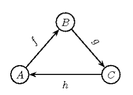
Figure 1: The Alternatives and the Choice Functions

We examine GSWFs satisfying (some of) the following conditions:

• Balance - A GSWF is balanced if the choice functions $f,g,$ and $h$ are balanced (i.e., satisfy $\mathbb{E}[f]=\mathbb{E}[g]=\mathbb{E}[h]=1/2$).

• Neutrality - A GSWF is neutral if it is invariant under permutations of the alternatives. In particular, this implies that the choice functions satisfy $f=g=h$, and that $f$ is balanced.

• Symmetry - We call a GSWF symmetric if it is invariant under a transitive group of permutations of the voters. In particular, this implies that the choice functions are far from a dictatorship.

• Monotonicity - A GSWF is monotone if the choice functions $f,g,$ and $h$ are monotone increasing.

The first direction in our paper is a generalization of the possible distributions of the individual preferences. In [11] it is assumed that the individual preferences are independent and uniformly distributed. We show that the results of [11] are valid (under some modifications) also for non-uniform distributions of the preferences, as long as the voters are independent, and for each ordering of the alternatives, the probability of the ordering is equal to the probability of the inverse ordering. We call such distributions even product distributions. In particular, we prove the following generalization of Theorem 5.1 of [11]:

Theorem 1.1.

Consider a GSWF on three alternatives satisfying the IIA condition. If the distribution of the preferences is an even product distribution such that the probability of each preference is positive, and the GSWF is neutral and symmetric, then the probability of irrational choice is bounded away from zero, independently of the number of the voters.

The second direction is obtaining new lower bounds on the probability of a rational choice for several classes of GSWFs. In particular, we prove the following conjecture raised in [11]:

Theorem 1.2.

Consider a GSWF on three alternatives satisfying the IIA condition. If the individual preferences are independent and uniformly distributed, and the GSWF is monotone and balanced, then the probability of a rational choice is at least 3/4.

The proof of this result relies on properties of the Bonamie-Beckner noise operator and uses the FKG inequality [7]. Furthermore, we establish a generalization of Theorem 1.2 to even product distributions of the individual preferences.

Finally, we consider the stability version of Arrow’s theorem presented in [11]. This version asserts that if a balanced GSWF on three alternatives satisfies the IIA condition and is at least $\epsilon$-far from being a dictatorship, then it leads to irrational choice with probability at least $C\cdot\epsilon$, for a universal constant $C$. Kalai asked whether his proof technique can be extended to an analytic proof of Arrow’s theorem without the neutrality assumption, or even to a stability version of Arrow’s theorem. (Such version would assert that for any $\epsilon>0$, there exists $\delta=\delta(\epsilon)$ such that if a GSWF on at least three candidates satisfies the IIA condition and is at least $\delta$-far from being a dictatorship and from not having all the orderings of the alternatives in its range, then the probability of irrational choice is at least $\epsilon$.)

We show that the neutrality assumption cannot be dropped completely from Kalai’s result, that is, there does not exist a stability version of Arrow’s theorem (with no additional assumptions) in which the dependence of $\delta(\epsilon)$ on $\epsilon$ is linear.

Theorem 1.3.

For all $\epsilon,K>0$ and $n=n(\epsilon,K)$ big enough, there exists a GSWF on three alternatives satisfying the IIA condition, such that:

1. Amongst any pair of alternatives, the probability of each alternative to be preferred by the society over the other alternative is at least $\eta=2^{-\epsilon n}/(n+1)$.

2. The probability of an irrational choice is less than $\eta/K$.

The example that proves Theorem 1.3 is a GSWF on three alternatives in which the choice functions $f,g,$ and $h$ are threshold functions (i.e., $(f(x)=1)\Leftrightarrow\left(\sum_{i=1}^{n}x_{i}\geq k\right)$ ), with expectations $\eta,1/2,$ and $1-\eta$.

After this paper was written, a stability version of Arrow’s theorem without additional assumptions was proved by Mossel [18]. In Mossel’s theorem, the dependence of $\delta$ on $\epsilon$ is $\delta=m^{2}\cdot\exp(C/\epsilon^{21})$ for a universal constant $C$, where $m$ is the number of alternatives. Recently, Keller [13] showed that the stability version holds for $\delta\approx Cm^{2}\cdot\epsilon^{8/9}$ where $C$ is a universal constant. Moreover, Keller showed that for small values of $\epsilon$, the example presented above (i.e., the threshold functions) is almost optimal: its probability of irrational choice is greater than the lower bound at most by a logarithmic factor (in $\epsilon$).

The paper is organized as follows: In Section 2 we recall some basic properties of the Fourier-Walsh expansion of functions on the discrete cube and of the Bonamie-Beckner noise operator. In Section 3 we generalize the results of [11] to even product distributions of the preferences and prove Theorem 4. In Section 4 we establish lower bounds on the probability of a rational choice for several classes of GSWFs and prove Theorem 1.2. In Section 5 we discuss Kalai’s stability version of Arrow’s theorem and prove Theorem 1.3.

2 Preliminaries

2.1 Fourier-Walsh Expansion of Functions on the Discrete Cube

Consider the discrete cube $\{0,1\}^{n}$ endowed with the uniform measure $\mu$. Denote the set of all real-valued functions on the discrete cube by $X$. The inner product of functions $f,g\in X$ is defined as usual as

$$\langle f,g\rangle=\mathbb{E}_{\mu}[fg]=\frac{1}{2^{n}}\sum_{x\in\{0,1\}^{n}}f(x)g(x).$$

This inner product induces a norm on $X$:

$$||f||_{2}=\sqrt{\langle f,f\rangle}=\sqrt{\mathbb{E}_{\mu}[f^{2}]}.$$

Consider the Rademacher functions $\{r_{i}\}_{i=1}^{n}$, defined as:

$$r_{i}(x_{1},\ldots,x_{n})=2x_{i}-1.$$

These functions constitute an orthonormal system in $X$. Moreover, this system can be completed to an orthonormal basis in $X$ by defining

$$r_{S}=\prod_{i\in S}r_{i},$$

for all $S\subset\{1,\ldots,n\}$. Every function $f\in X$ can be represented by its Fourier expansion with respect to the system $\{r_{S}\}_{S\subset\{1,\ldots,n\}}$:

$$f=\sum_{S\subset\{1,\ldots,n\}}\langle f,r_{S}\rangle r_{S}.$$

This representation is called the Fourier-Walsh expansion of $f$. The coefficients in this expansion are denoted by

$$\hat{f}(S)=\langle f,r_{S}\rangle,$$

and the level of the coefficient $\hat{f}(S)$ is $|S|$.

By the Parseval identity, for all $f\in X$,

$$\sum_{S\subset\{1,\ldots,n\}}\hat{f}(S)^{2}=||f||_{2}^{2}.$$

More generally, for all $f,g\in X$,

$$\langle f,g\rangle=\sum_{S\subset\{1,\ldots,n\}}\hat{f}(S)\hat{g}(S).$$

Following [11], we will be also interested in a biased version of the inner product, defined as follows:

Definition 2.1.

Let $f,g$ be two real-valued functions on the discrete cube, and let $-1\leq\delta\leq 1$. Define

$$\langle\langle f,g\rangle\rangle_{\delta}=\sum_{S\neq\emptyset}\hat{f}(S)\hat{g}(S)\delta^{|S|}.$$

Note that this definition slightly differs from the definition used in [11]. Finally, we note that for all $f\in X$,

$$\hat{f}(\emptyset)=\langle f,r_{\emptyset}\rangle=\mathbb{E}_{\mu}[f\cdot 1]=\mathbb{E}_{\mu}[f].$$

2.2 The Bonamie-Beckner Noise Operator

The noise operator, introduced in [4, 2], is defined in terms of the Fourier-Walsh expansion as follows:

Definition 2.2.

Consider a function $f$ on the discrete cube with a Fourier-Walsh expansion $f=\sum_{S}\hat{f}(S)r_{S}$. For $0\leq\epsilon\leq 1$, the noise operator $T_{\epsilon}$ applied to $f$ is

$$T_{\epsilon}f=\sum_{S}\epsilon^{|S|}\hat{f}(S)r_{S}.$$ (1)

It is well-known that one can arrive from $f$ to $T_{\epsilon}f$ by the following process: For any $x\in\{0,1\}^{n}$,

$$T_{\epsilon}f(x)=\mathbb{E}[f(x\oplus y)],$$ (2)

where $\oplus$ denotes coordinate-wise addition modulo $2$, and each coordinate of $y$ is chosen independently according to the distribution ${\bf Pr}[y_{i}=0]=(1+\epsilon)/2,{\bf Pr}[y_{i}=1]=(1-\epsilon)/2$. That is, each coordinate of $x$ is left unchanged with probability $\epsilon$ and is replaced by a random value with probability $1-\epsilon$, and then $f$ is evaluated on the result. Thus, $T_{\epsilon}f$ represents a noisy variant of $f$, and for this reason $T_{\epsilon}f$ is called “the noise operator”.

As pointed out by the anonymous referee, the noise operator can be defined in the same way (i.e., by Equation 1) also for $-1\leq\epsilon\leq 0$. Moreover, it can be easily shown that the basic property of the noise operator described above (i.e., Equation 2) also translates to the case $-1\leq\epsilon\leq 0$. That is, we still have

$$T_{\epsilon}f(x)=\mathbb{E}[f(x\oplus y)],$$

where each coordinate of $y$ is chosen independently according to the distribution ${\bf Pr}[y_{i}=0]=(1+\epsilon)/2,{\bf Pr}[y_{i}=1]=(1-\epsilon)/2$. Using this observation, we shall consider the noise operator for $-1\leq\epsilon\leq 1$.

3 The Probability of Rational Choice for a Non-Uniform Distribution of the Preferences

Throughout the paper we assume that the number of alternatives is three and denote the alternatives by $A,B,$ and $C$. Since (by assumption) the GSWF satisfies the IIA condition, the preference of the society between every pair of alternatives can be represented by a Boolean function on the discrete cube. Formally, given a profile, we consider the pair of alternatives $(A,B)$ and construct a binary vector $(x_{1},\ldots,x_{n})$ such that $x_{i}=1$ if the $i$-th voter prefers $A$ over $B$, and $x_{i}=0$ if the $i$-th voter prefers $B$ over $A$. We set $f(x_{1},\ldots,x_{n})=1$ if the entire society prefers $A$ over $B$ and $f(x_{1},\ldots,x_{n})=0$ if the society prefers $B$ over $A$. Note that the preference of the society between $A$ and $B$ is determined by $(x_{1},\ldots,x_{n})$, and hence $f$ is well-defined. Similarly, we define the Boolean functions $g$ and $h$ that represent the preferences between the pairs $(B,C)$ and $(C,A)$, respectively (see Figure 1).

Every profile is uniquely represented by the binary vector $(x_{1},\ldots,x_{n},y_{1},\ldots,y_{n},z_{1},\ldots,z_{n})$, where $(x_{i},y_{i},z_{i})$ represent the preferences of the $i$-th voter between $(A,B),(B,C)$, and $(C,A)$. We assume that the vectors $(x_{i},y_{i},z_{i})$ for different values of $i$ are independent (i.e., the preferences of the individual voters are independent), and that these vectors do not assume the values $(0,0,0)$ and $(1,1,1)$ (since otherwise the preferences of the $i$-th voter do not constitute an order relation). In [11], the distribution over the six possible values of $(x_{i},y_{i},z_{i})$ was assumed to be uniform. In our analysis, we consider the following distribution:

$${\bf Pr}[(x_{i},y_{i},z_{i})=(1,1,0)]=\alpha\qquad{\bf Pr}[(x_{i},y_{i},z_{i})=(0,1,1)]=\beta\qquad{\bf Pr}[(x_{i},y_{i},z_{i})=(1,0,1)]=\gamma$$

$${\bf Pr}[(x_{i},y_{i},z_{i})=(0,0,1)]=\alpha\qquad{\bf Pr}[(x_{i},y_{i},z_{i})=(1,0,0)]=\beta\qquad{\bf Pr}[(x_{i},y_{i},z_{i})=(0,1,0)]=\gamma,$$

where $\alpha+\beta+\gamma=1/2$. We call this distribution an even product distribution, and denote it by $D(\alpha,\beta,\gamma)$. The intuition behind the restrictions will be explained at the end of this section.

Theorem 3.1.

Consider a GSWF on three alternatives satisfying the IIA condition where the choice functions between the pairs of alternatives $(A,B),(B,C),$ and $(C,A)$ are $f,g,$ and $h$, respectively. If the distribution of the individual preferences is an even product distribution $D(\alpha,\beta,\gamma)$, as described above, then the probability of irrational choice is given by the formula:

$$W(f,g,h)=p_{1}p_{2}p_{3}+(1-p_{1})(1-p_{2})(1-p_{3})+\langle\langle f,g\rangle\rangle_{4\alpha-1}+\langle\langle g,h\rangle\rangle_{4\beta-1}+\langle\langle h,f\rangle\rangle_{4\gamma-1},$$ (3)

where $p_{1},p_{2},$ and $p_{3}$ are the expectations of $f,g,$ and $h$, respectively.

Remark 3.2.

Theorem 3.1 generalizes Theorem 3.1 of [11], which corresponds to the case $\alpha=\beta=\gamma=1/6$.

Proof: For a profile $(x,y,z)=(x_{1},\ldots,x_{n},y_{1},\ldots,y_{n},z_{1},\ldots,z_{n})$, the choice of the society is rational if and only if

$$f(x)g(y)h(z)+(1-f(x))(1-g(y))(1-h(z))=0.$$

Therefore, the probability of irrational choice is

$$W(f,g,h)=\sum_{(x,y,z)\in\{0,1\}^{3n}}{\bf Pr}[(x,y,z)]\Big{(}f(x)g(y)h(z)+(1-f(x))(1-g(y))(1-h(z))\Big{)},$$

where ${\bf Pr}[(x,y,z)]=\prod_{i}{\bf Pr}[(x_{i},y_{i},z_{i})]$, according to the distribution $D(\alpha,\beta,\gamma)$.

Consider the functions $F_{1},F_{2},F_{3}:\{0,1\}^{3n}\rightarrow\mathbb{R}$ defined by

$$F_{1}(x_{1},\ldots,x_{n},y_{1},\ldots,y_{n},z_{1},\ldots,z_{n})=f(x)g(y)h(z),$$

$$F_{2}(x_{1},\ldots,x_{n},y_{1},\ldots,y_{n},z_{1},\ldots,z_{n})=(1-f(x))(1-g(y))(1-h(z)),$$

$$F_{3}(x_{1},\ldots,x_{n},y_{1},\ldots,y_{n},z_{1},\ldots,z_{n})={\bf Pr}[(x,y,z)].$$

We have

$$W(f,g,h)=2^{3n}\langle F_{3},F_{1}+F_{2}\rangle,$$

and hence by the Parseval identity,

$$W(f,g,h)=2^{3n}\sum_{S\subset\{1,\ldots,3n\}}\hat{F}_{3}(S)(\hat{F}_{1}(S)+\hat{F}_{2}(S)).$$ (4)

Therefore, in order to compute the probability of rational choice it is sufficient to compute the Fourier-Walsh expansions of $F_{1},F_{2},$ and $F_{3}$.

In order to compute the expansions, we use the fact that if a function is a multiplication of functions on disjoint sets of variables, then its Fourier-Walsh expansion also has the same structure. Hence, if we denote $S=(S_{1},S_{2},S_{3})$, where $S_{1}$ represents $(x_{1},\ldots,x_{n})$, $S_{2}$ represents $(y_{1},\ldots,y_{n})$, and $S_{3}$ represents $(z_{1},\ldots,z_{n})$, then

$$\hat{F}_{1}(S)=\hat{f}(S_{1})\hat{g}(S_{2})\hat{h}(S_{3})\qquad\mbox{ and }\qquad\hat{F}_{2}(S)=\widehat{1-f}(S_{1})\widehat{1-g}(S_{2})\widehat{1-h}(S_{3}).$$

Similarly, since the individual preferences are independent, the Fourier-Walsh expansion of $F_{3}$ is determined by the Fourier-Walsh expansion of the functions $F_{4}^{i}:\{0,1\}^{3}\rightarrow\mathbb{R}$ defined by

$$F_{4}^{i}((x_{i},y_{i},z_{i}))={\bf Pr}[(x_{i},y_{i},z_{i})].$$

This expansion (presented below) can be found by direct computation.

$$\hat{F}_{4}^{i}(\emptyset)=1/8,\qquad\hat{F}_{4}^{i}(\{1\})=0,\qquad\hat{F}_{4}^{i}(\{2\})=0,\qquad\hat{F}_{4}^{i}(\{3\})=0,\qquad\hat{F}_{4}^{i}(\{1,2\})=(4\alpha-1)/8,$$

$$\hat{F}_{4}^{i}(\{2,3\})=(4\beta-1)/8,\qquad\hat{F}_{4}^{i}(\{1,3\})=(4\gamma-1)/8,\qquad\hat{F}_{4}^{i}(\{1,2,3\})=0.$$

Since the Fourier-Walsh coefficients of $F_{3}$ are multiplications of the corresponding coefficients of $\{F_{4}^{i}\}_{i=1}^{n}$, we have $\hat{F}_{3}(S)=0$, unless $S=(S_{1},S_{2},S_{3})$ has a special structure: Each $1\leq i\leq n$ is contained in either none or two of the sets $(S_{1},S_{2},S_{3})$. For such special sets $S$, the coefficients are given by the formula

$$\hat{F}_{3}(S)=\Big{(}\frac{1}{8}\Big{)}^{t_{1}}\Big{(}\frac{4\alpha-1}{8}\Big{)}^{t_{2}}\Big{(}\frac{4\beta-1}{8}\Big{)}^{t_{3}}\Big{(}\frac{4\gamma-1}{8}\Big{)}^{t_{4}},$$

where

$$t_{1}=\mbox{ the number of triples }(x_{i},y_{i},z_{i})\mbox{ equal to }(0,0,0),$$

$$t_{2}=\mbox{ the number of triples }(x_{i},y_{i},z_{i})\mbox{ equal to }(1,1,0),$$

$$t_{3}=\mbox{ the number of triples }(x_{i},y_{i},z_{i})\mbox{ equal to }(0,1,1),$$

$$t_{4}=\mbox{ the number of triples }(x_{i},y_{i},z_{i})\mbox{ equal to }(1,0,1).$$

Finally, we note that by the linearity of the Fourier transform, we have $\hat{f}(S_{1})=-(\widehat{1-f}(S_{1}))$ for all $S_{1}\neq\emptyset$, and the same for $g$ and $h$. Therefore, if $S_{1},S_{2},S_{3}\neq\emptyset$, then

$$\hat{F}_{1}(S)+\hat{F}_{2}(S)=0.$$

Combining the observations above, we get that the term

$$\hat{F}_{3}(S)(\hat{F}_{1}(S)+\hat{F}_{2}(S))$$

vanishes unless $S=(S_{1},S_{2},S_{3})$ has the following special structure: At least one of $S_{1},S_{2},S_{3}$ is empty, and each $i$ is contained in either none or two of $S_{1},S_{2},S_{3}$.

Assume that $S_{3}=\emptyset$, and thus $S_{1}=S_{2}$ (otherwise, there exists $i$ that is contained in only one of the sets $S_{1},S_{2},S_{3}$, and hence $\hat{F}_{3}(S)(\hat{F}_{1}(S)+\hat{F}_{2}(S))=0$). Assume also that $S_{1}\neq\emptyset$. We note that $\widehat{1-h}(\emptyset)=1-\hat{h}({\emptyset})$, and hence by the calculations above,

$$\hat{F}_{3}(S)(\hat{F}_{1}(S)+\hat{F}_{2}(S))=\Big{(}\frac{1}{8}\Big{)}^{n-|S_{1}|}\Big{(}\frac{4\alpha-1}{8}\Big{)}^{|S_{1}|}\hat{f}(S_{1})\hat{g}(S_{1})=\Big{(}\frac{1}{8}\Big{)}^{n}(4\alpha-1)^{|S_{1}|}\hat{f}(S_{1})\hat{g}(S_{1}).$$

If $S_{1}=S_{2}=S_{3}=\emptyset$, then

$$\hat{F}_{3}(S)(\hat{F}_{1}(S)+\hat{F}_{2}(S))=(1/8)^{n}(p_{1}p_{2}p_{3}+(1-p_{1})(1-p_{2})(1-p_{3})).$$

Therefore, summing over all the possible values of $S$ we get

$$\sum_{S\subset\{1,\ldots,3n\}}\hat{F}_{3}(S)(\hat{F}_{1}(S)+\hat{F}_{2}(S))=(1/8)^{n}\Big{(}p_{1}p_{2}p_{3}+(1-p_{1})(1-p_{2})(1-p_{3})+$$

$$+\sum_{S_{1}\neq\emptyset}(4\alpha-1)^{|S_{1}|}\hat{f}(S_{1})\hat{g}(S_{1})+\sum_{S_{2}\neq\emptyset}(4\beta-1)^{|S_{2}|}\hat{g}(S_{2})\hat{h}(S_{2})+\sum_{S_{3}\neq\emptyset}(4\gamma-1)^{|S_{3}|}\hat{f}(S_{3})\hat{h}(S_{3})\Big{)}=$$

$$=(1/8)^{n}\Big{(}p_{1}p_{2}p_{3}+(1-p_{1})(1-p_{2})(1-p_{3})+\langle\langle f,g\rangle\rangle_{4\alpha-1}+\langle\langle g,h\rangle\rangle_{4\beta-1}+\langle\langle h,f\rangle\rangle_{4\gamma-1}\Big{)},$$

and thus the assertion of the theorem follows from Equation (4). $\Box$

Using Theorem 3.1, some of the results of [11] and [16] can be generalized to even product distributions of the preferences. We present here two of the results.

Theorem 3.3.

Consider a GSWF on three alternatives satisfying the IIA condition. If the distribution of the preferences is an even product distribution $D(\alpha,\beta,\gamma)$ and the GSWF is neutral and symmetric, then the probability of an irrational choice satisfies the inequality

$$W(f,g,h)\geq(\frac{1}{4}-d_{m})(1+(4\alpha-1)^{3}+(4\beta-1)^{3}+(4\gamma-1)^{3})>0,$$ (5)

where $d_{m}\approx 1/(2\pi)$ is the sum of squares of the first-level Fourier-Walsh coefficients of the majority function. In particular, $W(f,g,h)$ is bounded away from zero.

Remark 3.4.

Theorem 3.3 generalizes Theorem 5.1 in [11], which corresponds to the case $\alpha=\beta=\gamma=1/6$.

In the proof of Theorem 3.3 we use the following technical lemma, obtained with the assistance of Tomer Schlank.

Lemma 3.5.

For any integer $k\geq 1$, and all $-1\leq x,y,z\leq 1$ such that $x+y+z=1$, we have

$$x^{3}+y^{3}+z^{3}\geq x^{2k+1}+y^{2k+1}+z^{2k+1}.$$ (6)

Proof: Denote $D=\{(x,y,z)\in[-1,1]^{3}|x+y+z=1\}$, and $f(x,y,z)=(x^{3}+y^{3}+z^{3})-(x^{2k+1}+y^{2k+1}+z^{2k+1})$. Since $D$ is compact and $f$ is continuous, $f$ obtains a minimum in $D$. We would like to show that $\min_{D}(f)=0$. First, we note that $f$ is identically zero on the boundary of $D$. Indeed, if $(x,y,z)\in\partial(D)$, then w.l.o.g., either $x=-1$ and then necessarily $y=z=1$, or $x=1$ and then $y=-z$. In both cases, $f(x,y,z)=0$. If $f$ attains its minimum in an internal point $(x_{0},y_{0},z_{0})\in D$, then by Lagrange multipliers, we have

$$3x_{0}^{2}-(2k+1)x_{0}^{2k}=3y_{0}^{2}-(2k+1)y_{0}^{2k}=3z_{0}^{2}-(2k+1)z_{0}^{2k}.$$

If $|x_{0}|\neq|y_{0}|$, the first equality is equivalent to:

$$\frac{3}{2k+1}=\frac{x_{0}^{2k}-y_{0}^{2k}}{x_{0}^{2}-y_{0}^{2}}=\sum_{l=0}^{k-1}(x_{0}^{2})^{l}(y_{0}^{2})^{k-1-l},$$ (7)

and similarly for the pairs $(x_{0},z_{0})$ and $(y_{0},z_{0})$. For a given $x_{0}$, the function $\sum_{l=0}^{k-1}(x_{0}^{2})^{l}(y_{0}^{2})^{k-1-l}$ is increasing as function of $y_{0}^{2}$. Hence, Equation (7) can be satisfied for both $(x_{0},y_{0})$ and $(x_{0},z_{0})$ only if $|y_{0}|=|z_{0}|$. Thus, an internal minimum point of $f$ in $D$ must satisfy at least one of the conditions $|x_{0}|=|y_{0}|$, $|x_{0}|=|z_{0}|$ or $|y_{0}|=|z_{0}|$. Assume, w.l.o.g., that $|x_{0}|=|y_{0}|$. If $x_{0}=-y_{0}$, then necessarily $z_{0}=1$, and thus $(x_{0},y_{0},z_{0})\in\partial(D)$. If $x_{0}=y_{0}$, then $z_{0}=1-2x_{0}$, and hence, Inequality (6) is reduced to:

$$2x_{0}^{3}+(1-2x_{0})^{3}\geq 2x_{0}^{2k+1}+(1-2x_{0})^{2k+1}.$$ (8)

Therefore, it is sufficient to prove Inequality (8) for all $0\leq x_{0}\leq 1$. Note that the inequality holds trivially for $x_{0}\leq 1/2$. Let $g(t)=t^{3}-t^{2k+1}$, and denote $\delta=1-x$. By Inequality (8), it is sufficient to prove that for all $0\leq\delta\leq 1/2$,

$$2g(1-\delta)\geq g(1-2\delta).$$ (9)

We use the following two properties of $g(t)$:

1. $g(t)$ is nonnegative for all $0\leq t\leq 1$. Furthermore, $g$ is monotone increasing for $0<t<t_{0}$ and monotone decreasing for $t_{0}<t<1$, where $t_{0}=(\frac{3}{2k+1})^{1/(2k-2)}$.

2. $g(t)$ is convex in the domain $0<t<t_{1}$, and concave in the domain $t_{1}<t<1$, where $t_{1}=(\frac{6}{2k(2k+1)})^{1/(2k-2)}$.

Since $g(1)=0$, Inequality (9) follows from the concavity of $g$ whenever $1-2\delta\geq t_{1}$. Furthermore, when $1-\delta\leq t_{0}$, the inequality follows immediately from the monotonicity and nonnegativity of $g$ in that domain. The only remaining case is when $1-2\delta<t_{1}$ and $1-\delta>t_{0}$ (or equivalently, $(1-t_{1})/2<\delta<1-t_{0}$. We note that this domain may be empty, and in this case we are already done by the previous considerations). In this case, by the monotonicity properties of $g$ we have $g(1-\delta)>g((1+t_{1})/2)$ (since $t_{0}<1-\delta<(1+t_{1})/2$), and $g(1-2\delta)<g(t_{1})$ (since $1-2\delta<t_{1}<t_{0}$). Therefore,

$$2g(1-\delta)-g(1-2\delta)>2g((1+t_{1})/2)-g(t_{1})\geq 0,$$

where the last inequality follows from the concavity of $g(t)$ for $t_{1}<t<1$. This completes the proof. $\Box$

Proof of Theorem 3.3. By assumption, the GSWF is neutral, and hence, balanced. Therefore, by Theorem 3.1, the probability of irrational choice in our case is

$$W(f,g,h)=1/4+\langle\langle f,g\rangle\rangle_{4\alpha-1}+\langle\langle g,h\rangle\rangle_{4\beta-1}+\langle\langle h,f\rangle\rangle_{4\gamma-1}.$$

Since the GSWF is neutral and symmetric, we have $f=g=h$, and all the Fourier-Walsh coefficients of $f$ on the even non-zero levels vanish (see [11], Proof of Theorem 5.1). Thus,

$$W(f,g,h)=1/4+\sum_{|S|\mbox{ odd }}\hat{f}(S)^{2}(4\alpha-1)^{|S|}+\sum_{|S|\mbox{ odd }}\hat{f}(S)^{2}(4\beta-1)^{|S|}+\sum_{|S|\mbox{ odd }}\hat{f}(S)^{2}(4\gamma-1)^{|S|}=$$

$$=1/4+\sum_{k=0}^{\lceil n/2\rceil-1}\Big{[}((4\alpha-1)^{2k+1}+(4\beta-1)^{2k+1}+(4\gamma-1)^{2k+1})\sum_{|S|=2k+1}\hat{f}(S)^{2}\Big{]}=$$

$$=1/4-\sum_{|S|=1}\hat{f}(S)^{2}+\sum_{k=1}^{\lceil n/2\rceil-1}((4\alpha-1)^{2k+1}+(4\beta-1)^{2k+1}+(4\gamma-1)^{2k+1})\sum_{|S|=2k+1}\hat{f}(S)^{2},$$

where the last equality follows from the relation $\alpha+\beta+\gamma=1/2$. Since for every $k$ the expression $\sum_{|S|=2k+1}\hat{f}(S)^{2}$ is non-negative, and since by Lemma 3.5, for all $k\geq 1$,

$$(4\alpha-1)^{2k+1}+(4\beta-1)^{2k+1}+(4\gamma-1)^{2k+1}\geq(4\alpha-1)^{3}+(4\beta-1)^{3}+(4\gamma-1)^{3},$$

it follows that

$$W(f,g,h)\geq 1/4-\sum_{|S|=1}\hat{f}(S)^{2}+\left((4\alpha-1)^{3}+(4\beta-1)^{3}+(4\gamma-1)^{3}\right)\sum_{|S|>1}\hat{f}(S)^{2}=$$

$$=(1/4-\sum_{|S|=1}\hat{f}(S)^{2})(1+(4\alpha-1)^{3}+(4\beta-1)^{3}+(4\gamma-1)^{3}),$$

where the last equality follows from the Parseval identity. Since amongst the symmetric neutral functions, the expression $\sum_{|S|=1}\hat{f}(S)^{2}$ is maximized for the majority function (see proof of Theorem 5.1 in [11]), we get

$$W(f,g,h)\geq(\frac{1}{4}-d_{m})(1+(4\alpha-1)^{3}+(4\beta-1)^{3}+(4\gamma-1)^{3}),$$

and thus it is only left to show that

$$(4\alpha-1)^{3}+(4\beta-1)^{3}+(4\gamma-1)^{3}>-1.$$ (10)

This claim is trivial for $\alpha,\beta,\gamma\leq 1/4$, since in that case

$$(4\alpha-1)^{3}+(4\beta-1)^{3}+(4\gamma-1)^{3}>(4\alpha-1)+(4\beta-1)+(4\gamma-1)=-1.$$

Hence, assume that $\gamma>1/4$, and write $\gamma=1/2-\alpha-\beta$ (and thus $4\gamma-1=1-4\alpha-4\beta$). Inequality (10) is equivalent to

$$(1-4\alpha)^{3}+(1-4\beta)^{3}<1+(1-4\alpha-4\beta)^{3},$$

that follows from the strict convexity of the function $F(t)=t^{3}$ on $[0,1]$. This completes the proof of Theorem 3.3. $\square$

The second result is a combination of Theorem 3.1 with the following proposition, which is an easy consequence of the “Majority is stablest” theorem [16]:

Proposition 3.6.

Let $0\leq\rho\leq 1$ and let $\epsilon>0$. There exists $n_{0}=n_{0}(\rho,\epsilon)$ such that for all $n>n_{0}$, if $f:\{0,1\}^{n}\rightarrow[0,1]$ is symmetric and balanced then

$$\langle\langle f,f\rangle\rangle_{\rho}=\sum_{S\neq\emptyset}\hat{f}(S)^{2}\rho^{|S|}\leq\frac{1}{2\pi}\arcsin\rho+\epsilon.$$

Corollary 3.7.

Consider a GSWF on three alternatives, where the distribution of the preferences is an even product distribution $D(\alpha,\beta,\gamma)$ with $\alpha,\beta,\gamma\leq 1/4$. Then for all $\epsilon>0$ there exists $n_{0}=n_{0}(\epsilon,\alpha,\beta,\gamma)$ such that if the number of voters is $n>n_{0}$ and the GSWF is neutral, symmetric, and satisfies the IIA condition, then the probability of a rational choice is at most $p+\epsilon$, where $p$ is the probability of a rational choice for the majority GSWF on $n$ voters and three alternatives.

Proof: Similarly to the proof of Theorem 3.3, if $\alpha,\beta,\gamma\leq 1/4$ then

$$W(f,g,h)=1/4+\sum_{|S|\mbox{ odd }}\hat{f}(S)^{2}(4\alpha-1)^{|S|}+\sum_{|S|\mbox{ odd }}\hat{f}(S)^{2}(4\beta-1)^{|S|}+\sum_{|S|\mbox{ odd }}\hat{f}(S)^{2}(4\gamma-1)^{|S|}=$$

$$=1/4-\sum_{|S|\mbox{ odd }}\hat{f}(S)^{2}|4\alpha-1|^{|S|}-\sum_{|S|\mbox{ odd }}\hat{f}(S)^{2}|4\beta-1|^{|S|}-\sum_{|S|\mbox{ odd }}\hat{f}(S)^{2}|4\gamma-1|^{|S|}=$$

$$=1/4-\langle\langle f,f\rangle\rangle_{|4\alpha-1|}-\langle\langle f,f\rangle\rangle_{|4\beta-1|}-\langle\langle f,f\rangle\rangle_{|4\gamma-1|}.$$

Hence, by Proposition 3.6, for every $\epsilon>0$ there exists $n_{0}=n_{0}(\epsilon,\alpha,\beta,\gamma)$ such that for every GSWF on $n>n_{0}$ voters satisfying the assumptions of the corollary,

$$W(f,g,h)\geq 1/4-\frac{1}{2\pi}\arcsin(|4\alpha-1|)-\frac{1}{2\pi}\arcsin(|4\beta-1|)-\frac{1}{2\pi}\arcsin(|4\gamma-1|)-\epsilon.$$

Finally, since for the majority GSWF $F_{n}$ on $n$ voters we have, for all $0\leq\rho\leq 1$,

$$\lim_{n\rightarrow\infty}\langle\langle F_{n},F_{n}\rangle\rangle_{\rho}=\frac{1}{2\pi}\arcsin\rho$$

(see [16], Section 4), the assertion of the corollary follows. $\Box$

Remark 3.8.

Corollary 3.7 is proved in [16] for a uniform distribution of the preferences, as a corollary of the “Majority is Stablest” theorem.

Remark 3.9.

Conjecture 8.1 of [11] asserts that for every distribution of the preferences (and even for more than three alternatives), the probability of a rational choice for GSWFs that are neutral, symmetric, and satisfy the IIA condition, is maximized for the majority function. Hence, Corollary 3.7 proves in the asymptotic sense (i.e., for a sufficiently large $n$) a special case of the conjecture.

We conclude this section by explaining the restriction on the distribution of the individual preferences. The proof of Theorem 3.1 crucially depends on the fact that $\hat{F}_{4}^{i}(\{j\})$ vanishes for $j=1,2,3$. This condition holds if and only if the probabilities of the preferences satisfy the following three equations:

$${\bf Pr}[1,0,0]+{\bf Pr}[1,1,0]+{\bf Pr}[1,0,1]-{\bf Pr}[0,1,0]-{\bf Pr}[0,0,1]-{\bf Pr}[0,1,1]=0,$$

$${\bf Pr}[0,1,0]+{\bf Pr}[1,1,0]+{\bf Pr}[0,1,1]-{\bf Pr}[1,0,0]-{\bf Pr}[0,0,1]-{\bf Pr}[1,0,1]=0,$$

$${\bf Pr}[0,0,1]+{\bf Pr}[1,0,1]+{\bf Pr}[0,1,1]-{\bf Pr}[1,0,0]-{\bf Pr}[0,1,0]-{\bf Pr}[1,1,0]=0,$$

where ${\bf Pr}[a,b,c]$ is a shorthand for ${\bf Pr}[(x_{i},y_{i},z_{i})=(a,b,c)]$. Summing the first two equations we get

$$2{\bf Pr}[1,1,0]-2{\bf Pr}[0,0,1]=0,$$

and similarly by summing the two other pairs of equations we get ${\bf Pr}[1,0,1]={\bf Pr}[0,1,0]$ and ${\bf Pr}[0,1,1]={\bf Pr}[1,0,0]$. Finally, since all the probabilities sum up to one, we get ${\bf Pr}[1,0,0]+{\bf Pr}[0,1,0]+{\bf Pr}[0,0,1]=1/2$, and this completes the restrictions described above. It is challenging to generalize Theorem 3.1 to more general distributions on the preferences, but the expression $\sum_{S\subset\{1,\ldots,3n\}}\hat{F}_{3}(S)(\hat{F}_{1}(S)+\hat{F}_{2}(S))$ seems hard to compute in the general case.

4 Lower Bounds on the Probability of Rational Choice

In this section we establish lower bounds on the probability of a rational choice for two classes of GSWFs: monotone balanced functions and general balanced functions.

4.1 Monotone Balanced GSWFs

Definition 4.1.

A function $f:\{0,1\}^{n}\rightarrow\mathbb{R}$ is monotone increasing if for all $x=(x_{1},\ldots,x_{n})$ and $y=(y_{1},\ldots,y_{n})$,

$$(\forall i:x_{i}\leq y_{i})\Rightarrow(f(x)\leq f(y)).$$

Similarly, a function is monotone decreasing if

$$(\forall i:x_{i}\leq y_{i})\Rightarrow(f(x)\geq f(y)).$$

Theorem 1.2 is a special case of the following, more general, result:

Theorem 4.2.

Consider a GSWF on three alternatives satisfying the IIA condition where the choice functions between the pairs of alternatives $(A,B),(B,C),$ and $(C,A)$, denoted by $f,g,$ and $h$, respectively, are monotone increasing. If the distribution of the preferences is an even product distribution satisfying $\alpha,\beta,\gamma\leq 1/4$ (and in particular, if the preferences are uniformly distributed) then the probability of irrational choice satisfies:

$$W(f,g,h)\leq p_{1}p_{2}p_{3}+(1-p_{1})(1-p_{2})(1-p_{3}),$$ (11)

where $p_{1},p_{2},$ and $p_{3}$ are the expectations of $f,g,$ and $h$, respectively.

Remark 4.3.

The assertion of Theorem 4.2 is tight, as can be seen in the following example: Assume that $f$ depends only on the first voter, $g$ depends only on the second voter, and $h$ depends only on the third voter. Then clearly, for all $-1\leq\delta\leq 1$,

$$\langle\langle f,g\rangle\rangle_{\delta}=\langle\langle g,h\rangle\rangle_{\delta}=\langle\langle h,f\rangle\rangle_{\delta}=0,$$

and thus,

$$W(f,g,h)=p_{1}p_{2}p_{3}+(1-p_{1})(1-p_{2})(1-p_{3}),$$

where $p_{1},p_{2},$ and $p_{3}$ are the expectations of $f,g,$ and $h$, respectively.

By Theorem 3.1, the assertion of Theorem 4.2 is an immediate consequence of the following proposition:

Proposition 4.4.

For any two monotone increasing Boolean functions $f$ and $g$, and for every $-1\leq\delta\leq 1$,

$$\frac{1}{\delta}\langle\langle f,g\rangle\rangle_{\delta}\geq 0.$$ (12)

The proof of Proposition 12 uses properties of the Bonamie-Beckner noise operator and the FKG correlation inequality [7]. For the reader’s convenience, we recall the statement of the FKG inequality in the special case of the uniform measure on the discrete cube.

Theorem 4.5 (Fortuin, Kasteleyn, and Ginibre).

Consider the discrete cube $\{0,1\}^{n}$ endowed with the uniform measure $\mu$, and let $f,g:\{0,1\}^{n}\rightarrow\mathbb{R}$. Then:

1. If both $f$ and $g$ are monotone increasing, then $\mathbb{E}_{\mu}[fg]\geq\mathbb{E}_{\mu}[f]\mathbb{E}_{\mu}[g]$.

2. If $f$ is monotone increasing and $g$ is monotone decreasing, then $\mathbb{E}_{\mu}[fg]\leq\mathbb{E}_{\mu}[f]\mathbb{E}_{\mu}[g]$.

Proof of Proposition 12. By the definition of the noise operator $T_{\epsilon}$, we have

$$\frac{1}{\delta}\langle\langle f,g\rangle\rangle_{\delta}=\frac{1}{\delta}\sum_{S\neq\emptyset}\delta^{|S|}\hat{f}(S)\hat{g}(S)=\frac{1}{\delta}\sum_{S\neq\emptyset}\widehat{T_{\delta}f}(S)\hat{g}(S).$$

By the Parseval identity,

$$\frac{1}{\delta}\sum_{S\neq\emptyset}\widehat{T_{\delta}f}(S)\hat{g}(S)=\frac{1}{\delta}\Big{(}\sum_{S}\widehat{T_{\delta}f}(S)\hat{g}(S)-\widehat{T_{\delta}f}(\emptyset)\hat{g}(\emptyset)\Big{)}=\frac{1}{\delta}(\mathbb{E}_{\mu}[T_{\delta}f\cdot g]-\mathbb{E}_{\mu}[T_{\delta}f]\mathbb{E}_{\mu}[g]).$$

Hence, Inequality (12) is equivalent to the inequality:

$$\frac{1}{\delta}(\mathbb{E}_{\mu}[T_{\delta}f\cdot g]-\mathbb{E}_{\mu}[T_{\delta}f]\mathbb{E}_{\mu}[g])\geq 0.$$ (13)

Since the function $g$ is monotone increasing, Inequality (13) will follow from the FKG inequality, once we show that $T_{\delta}f$ is monotone increasing if $0\leq\delta\leq 1$, and monotone decreasing if $-1\leq\delta\leq 0$. We show the case of $-1\leq\delta\leq 0$ (the case of positive $\delta$ is similar).

Without loss of generality, it is sufficient to prove that for all $(x_{2},\ldots,x_{n})\in\{0,1\}^{n-1}$,

$$T_{\delta}f(0,x_{2},\ldots,x_{n})\geq T_{\delta}f(1,x_{2},\ldots,x_{n}).$$ (14)

Using the equivalent definition of the noise operator presented in Section 2.2 (i.e., Equation (2)),

$$T_{\delta}f(x_{1},x_{2},\ldots,x_{n})=\mathbb{E}[f((x_{1},x_{2},\ldots,x_{n})\oplus(y_{1},\ldots,y_{n}))],$$

where each $y_{i}$ is distributed according to the distribution ${\bf Pr}[y_{i}=0]=(1+\delta)/2,{\bf Pr}[y_{i}=1]=(1-\delta)/2$, independently of other $y_{i}$’s. Thus, we have to show that for all $(x_{2},\ldots,x_{n})\in\{0,1\}^{n-1}$,

$$\mathbb{E}[f((y_{1},x_{2}\oplus y_{2},\ldots,x_{n}\oplus y_{n}))]\geq\mathbb{E}[f((1\oplus y_{1},x_{2}\oplus y_{2},\ldots,x_{n}\oplus y_{n}))].$$

Therefore, it is sufficient to show that for each $(z_{2},\ldots,z_{n})\in\{0,1\}^{n-1}$,

$$\mathbb{E}_{y_{1}}[f((y_{1},z_{2},\ldots,z_{n}))]\geq\mathbb{E}_{y_{1}}[f((1\oplus y_{1},z_{2},\ldots,z_{n}))],$$

or equivalently

$$\frac{1+\delta}{2}f(0,z_{2},\ldots,z_{n})+\frac{1-\delta}{2}f(1,z_{2},\ldots,z_{n})\geq\frac{1-\delta}{2}f(0,z_{2},\ldots,z_{n})+\frac{1+\delta}{2}f(1,z_{2},\ldots,z_{n}).$$

This inequality indeed follows from the monotonicity of $f$, since $\delta\leq 0$. This completes the proof of Proposition 12. $\square$

For a general even product distribution of the preferences, the probability of a rational choice for balanced monotone choice functions can be as low as $1/2$ (compared to $3/4$ in the case $\alpha,\beta,\gamma\leq 1/4$). An example in which the probability is $1/2$ is the following:

Example    Assume that the distribution on the preferences is: ${\bf Pr}[(x_{i},y_{i},z_{i})=(1,1,0)]=1/2$ and ${\bf Pr}[(x_{i},y_{i},z_{i})=(0,0,1)]=1/2$, while the probability of the other preferences is zero (i.e., $\alpha=1/2$ and $\beta=\gamma=0$). The choice functions $f$ and $g$ are a dictatorship of the first voter, and $h$ is a dictatorship of the second voter. Then it is easy to see that $W(f,g,h)=1/2$.

It can be shown that $1/2$ is a lower bound for the probability of a rational choice in our case. Indeed, by Theorem 3.1, for balanced choice functions we have

$$W(f,g,h)=1/4+\langle\langle f,g\rangle\rangle_{4\alpha-1}+\langle\langle g,h\rangle\rangle_{4\beta-1}+\langle\langle h,f\rangle\rangle_{4\gamma-1}.$$ (15)

By Proposition 12, an expression of the form $\langle\langle f,g\rangle\rangle_{4\alpha-1}$ can be positive only if $\alpha>1/4$. Since in our distribution $\alpha+\beta+\gamma=1/2$, at most one of the expressions of this form appearing in Equation (15) is positive. By the Cauchy-Schwarz inequality,

$$\langle\langle f,g\rangle\rangle_{4\alpha-1}=\sum_{S\neq\emptyset}\hat{f}(S)\hat{g}(S)(4\alpha-1)^{|S|}\leq 1/4,$$

and similarly for $\beta$ and $\gamma$. Therefore, $W(f,g,h)\leq 1/4+(1/4+0+0)=1/2$.

The probability of a rational choice is equal to $1/2$ if and only if $\langle\langle f,g\rangle\rangle_{4\alpha-1}=1/4$, and $\langle\langle g,h\rangle\rangle_{4\beta-1}=\langle\langle h,f\rangle\rangle_{4\gamma-1}=0$ (up to a permutation between $\alpha,\beta,$ and $\gamma$). By the Cauchy-Schwarz inequality, this occurs if and only if the following three conditions are satisfied:

• The distribution of the preferences is $\alpha=1/2,\beta=\gamma=0$.

• The choice functions $f,g$ satisfy $f=g$.

• The choice function $h$ is independent of $f$, in the following sense: The set of voters $\{1,\ldots,n\}$ can be partitioned into two disjoint sets $A$ and $B$ such that the output of $f$ depends only on the elements of $A$, and the output of $h$ depends only on the elements of $B$.

4.2 General Balanced GSWFs

In [11] it is stated (Proposition 5.2) that if the preferences are uniformly distributed, then the lower bound for the probability of rational choice for general balanced GSWFs is $2/3$. However, the proof sketched in [11] is insufficient, and it is not even clear that the lower bound itself is correct. In this subsection we prove a weaker lower bound, and discuss its tightness.

Theorem 4.6.

Consider a GSWF on three alternatives satisfying the IIA condition such that the choice functions between the pairs of alternatives are balanced. If the preferences are uniformly distributed then the probability of a rational choice is at least $5/8$.

Proof: Consider the Fourier-Walsh expansions of the choice functions $f,g$, and $h$. Let

$$\sum_{i=1}^{n}\hat{f}(\{i\})^{2}=a,\qquad\sum_{i=1}^{n}\hat{g}(\{i\})^{2}=b,\qquad\sum_{i=1}^{n}\hat{h}(\{i\})^{2}=c.$$

Since $f,g,$ and $h$ are balanced, then by the Parseval identity

$$\sum_{|S|>1}\hat{f}(S)^{2}=1/4-a,\qquad\sum_{|S|>1}\hat{g}(S)^{2}=1/4-b,\qquad\sum_{|S|>1}\hat{h}(S)^{2}=1/4-c.$$

Recall that by Theorem 3.1, in our case

$$W(f,g,h)=1/4+\langle\langle f,g\rangle\rangle_{-1/3}+\langle\langle g,h\rangle\rangle_{-1/3}+\langle\langle h,f\rangle\rangle_{-1/3}.$$ (16)

We have

$$\langle\langle f,g\rangle\rangle_{-1/3}+\langle\langle g,h\rangle\rangle_{-1/3}+\langle\langle h,f\rangle\rangle_{-1/3}=\sum_{|S|>0}\Big{(}\hat{f}(S)\hat{g}(S)+\hat{g}(S)\hat{h}(S)+\hat{h}(S)\hat{f}(S)\Big{)}(-1/3)^{|S|}=$$

$$=-\frac{1}{3}\sum_{|S|=1}\Big{(}\hat{f}(S)\hat{g}(S)+\hat{g}(S)\hat{h}(S)+\hat{h}(S)\hat{f}(S)\Big{)}+\sum_{|S|>1}\Big{(}\hat{f}(S)\hat{g}(S)+\hat{g}(S)\hat{h}(S)+\hat{h}(S)\hat{f}(S)\Big{)}(-1/3)^{|S|}\leq$$

$$\leq-\frac{1}{3}\sum_{|S|=1}\Big{(}\hat{f}(S)\hat{g}(S)+\hat{g}(S)\hat{h}(S)+\hat{h}(S)\hat{f}(S)\Big{)}+\frac{1}{9}\sum_{|S|>1}\Big{|}\hat{f}(S)\hat{g}(S)+\hat{g}(S)\hat{h}(S)+\hat{h}(S)\hat{f}(S)\Big{|}.$$

In order to bound the first summand, we use the elementary inequality

$$-(xy+yz+xz)\leq(x^{2}+y^{2}+z^{2})/2.$$

We get

$$-\frac{1}{3}\sum_{|S|=1}\Big{(}\hat{f}(S)\hat{g}(S)+\hat{g}(S)\hat{h}(S)+\hat{h}(S)\hat{f}(S)\Big{)}=-\frac{1}{3}\sum_{i=1}^{n}\Big{(}\hat{f}(\{i\})\hat{g}(\{i\})+\hat{g}(\{i\})\hat{h}(\{i\})+\hat{h}(\{i\})\hat{f}(\{i\})\Big{)}\leq$$

$$\leq\frac{1}{6}\sum_{i=1}^{n}\Big{(}\hat{f}(\{i\})^{2}+\hat{g}(\{i\})^{2}+\hat{h}(\{i\})^{2}\Big{)}=\frac{a+b+c}{6}.$$

In order to bound the second summand, we use the Cauchy-Schwarz inequality and the inequality between the arithmetic and the geometric means. Let

$$\tilde{f}=\sum_{|S|>1}|\hat{f}(S)|r_{S},\qquad\tilde{g}=\sum_{|S|>1}|\hat{g}(S)|r_{S}.$$

Applying the Cauchy-Schwarz inequality and the Parseval identity we get

$$\sum_{|S|>1}|\hat{f}(S)\hat{g}(S)|=\langle\tilde{f},\tilde{g}\rangle\leq||\tilde{f}||_{2}||\tilde{g}||_{2}=\sqrt{(1/4-a)(1/4-b)}\leq 1/4-(a+b)/2,$$

where the last inequality follows from the inequality between the arithmetic and the geometric means. Applying the same inequalities to the pairs $(g,h)$ and $(h,f)$, we get

$$\frac{1}{9}\sum_{|S|>1}\Big{|}\hat{f}(S)\hat{g}(S)+\hat{g}(S)\hat{h}(S)+\hat{h}(S)\hat{f}(S)\Big{|}\leq$$

$$\leq\frac{1}{9}\Big{(}\frac{1}{4}-\frac{a+b}{2}+\frac{1}{4}-\frac{b+c}{2}+\frac{1}{4}-\frac{c+a}{2}\Big{)}=\frac{1}{12}-\frac{a+b+c}{9}.$$

Combining the bounds obtained above, we get

$$-\frac{1}{3}\sum_{|S|=1}\Big{(}\hat{f}(S)\hat{g}(S)+\hat{g}(S)\hat{h}(S)+\hat{h}(S)\hat{f}(S)\Big{)}+\frac{1}{9}\sum_{|S|>1}\Big{|}\hat{f}(S)\hat{g}(S)+\hat{g}(S)\hat{h}(S)+\hat{h}(S)\hat{f}(S)\Big{|}\leq$$

$$\leq\frac{a+b+c}{6}+\frac{1}{12}-\frac{a+b+c}{9}=\frac{1}{12}+\frac{a+b+c}{18}.$$

Substitution to Equation (16) yields:

$$W(f,g,h)\leq 1/4+1/12+(a+b+c)/18=1/3+(a+b+c)/18.$$

Finally, since by the Parseval identity we have $0\leq a,b,c\leq 1/4$, the maximum in the right hand side is obtained for $a=b=c=1/4$, and thus,

$$W(f,g,h)\leq 1/3+(3/4)/18=3/8,$$

as asserted. $\Box$

The tightness of the lower bound in Theorem 4.6 is not clear to us. The example presented in [11] yields the value $W(f,g,h)=1/3$, where all the Fourier-Walsh coefficients of $f,g,$ and $h$ are concentrated on the second level. Another example yielding the same value of $W(f,g,h)$ is

$$f(x_{1},\ldots,x_{n})=x_{i},\qquad g(x_{1},\ldots,x_{n})=x_{i},\qquad h(x_{1},\ldots,x_{n})=1-x_{i},$$

for any $1\leq i\leq n$. In this example, all the weight of $f,g,$ and $h$ is concentrated on the first level. It seems possible that the correct lower bound is $2/3$, as asserted in [11]. However, in order to prove this bound, one has to exploit the fact that the choice functions are Boolean, as can be seen in the following example:

Example    Let $f,g,h$ be defined by $\hat{f}(\emptyset)=\hat{g}(\emptyset)=\hat{h}(\emptyset)=1/2$ and

$$\hat{f}({i})=\frac{2}{2\sqrt{6}},\qquad\hat{f}({j})=-\frac{1}{2\sqrt{6}},\qquad\hat{f}({k})=-\frac{1}{2\sqrt{6}},$$

$$\hat{g}({i})=-\frac{1}{2\sqrt{6}},\qquad\hat{g}({j})=\frac{2}{2\sqrt{6}},\qquad\hat{g}({k})=-\frac{1}{2\sqrt{6}},$$

$$\hat{h}({i})=-\frac{1}{2\sqrt{6}},\qquad\hat{h}({j})=-\frac{1}{2\sqrt{6}},\qquad\hat{h}({k})=\frac{2}{2\sqrt{6}},$$

for $1\leq i<j<k\leq n$. The rest of the Fourier-Walsh coefficients of $f,g,$ and $h$ are zero. Since

$$\sum_{S\neq\emptyset}\hat{f}(S)^{2}=\sum_{S\neq\emptyset}\hat{g}(S)^{2}=\sum_{S\neq\emptyset}\hat{h}(S)^{2}=1/4,$$

the functions $f,g,$ and $h$ “look like” balanced functions from the Fourier-theoretic point of view. Nevertheless, $W(f,g,h)=3/8$, which agrees with the lower bound of Theorem 4.6. This shows that in order to improve Theorem 4.6, we have to use the fact that $f,g,$ and $h$ are Boolean functions.

5 Upper Bounds on the Probability of Rational Choice

Throughout this section we assume that the preferences are uniformly distributed.

In this section we discuss Kalai’s [11] proof of Arrow’s Impossibility theorem for neutral GSWFs on three alternatives. First we discuss the possibility of extending Kalai’s proof to other special cases of Arrow’s theorem, and then we discuss the stability version of the theorem proved by Kalai (for neutral GSWFs).

5.1 Extending Kalai’s Proof to Other Special Cases of Arrow’s Theorem

Kalai’s proof uses the Fourier-theoretic formula for the probability of irrational choice for GSWFs on three altrenatives satisfying the IIA condition (Theorem 3.1). For a balanced GSWF, the formula reads:

$$W(f,g,h)=1/4+\langle\langle f,g\rangle\rangle_{-1/3}+\langle\langle g,h\rangle\rangle_{-1/3}+\langle\langle h,f\rangle\rangle_{-1/3}.$$ (17)

Define

$$\tilde{f}=\sum_{S\neq\emptyset}\hat{f}(S)r_{S},\qquad\overline{g}=\sum_{S\neq\emptyset}\hat{g}(S)(-1/3)^{|S|}r_{S}.$$

Note that since $f$ and $g$ are balanced, by the Parseval identity $||\tilde{f}||_{2}=1/2$ and $||\overline{g}||_{2}\leq 1/6$. Therefore, by the Cauchy-Schwarz inequality,

$$|\langle\langle f,g\rangle\rangle_{-1/3}|=|\langle\tilde{f},\overline{g}\rangle|\leq||\tilde{f}||_{2}||\overline{g}||_{2}\leq 1/12,$$

and it can be shown that equality can hold only if all the Fourier-Walsh coefficients of $f$ and of $g$ are on the first level. Then, it can be further shown that $W(f,g,h)=0$ can hold only if $f,g,$ and $h$ are dictatorships of the same voter, and this completes the proof of the theorem.

It was suggested in [11] to use the same reasoning in the non-balanced case. Such generalization is possible if $p_{1},p_{2},$ and $p_{3}$, the expectations of $f,g,$ and $h$, satisfy some condition described in [11]. However, this condition is not satisfied in many cases, e.g., for $p_{1}=p_{2}=1/5$ and $p_{3}=1$, as noted in [11]. Kalai [12] suggested to improve the upper bound $||\overline{g}||_{2}\leq 1/6$ (or, more generally, $||\overline{g}||_{2}\leq\sqrt{p_{2}(1-p_{2})}/3$) used in the proof by using the Bonamie-Beckner hypercontractive inequality [4, 2].

We show by an example that this proof strategy, even using the hypercontractive inequality, cannot lead to a complete proof of Arrow’s theorem. The example shows that if the biased inner product $\langle\langle f,g\rangle\rangle_{-1/3}$ is replaced by

$$\langle\langle f,g\rangle\rangle^{\prime}_{-1/3}=-\sum_{S\neq\emptyset}|\hat{f}(S)\hat{g}(S)(-1/3)^{|S|}|,$$

then there exist functions $f,g,h$ such that

$$W^{\prime}(f,g,h)=p_{1}p_{2}p_{3}+(1-p_{1})(1-p_{2})(1-p_{3})+\langle\langle f,g\rangle\rangle^{\prime}_{-1/3}+\langle\langle g,h\rangle\rangle^{\prime}_{-1/3}+\langle\langle h,f\rangle\rangle^{\prime}_{-1/3}<0.$$

Hence, a proof of Arrow’s theorem using Equation (17) cannot ignore the sign of the Fourier-Walsh coefficients of the choice functions.

The example uses the notion of a dual function:

Definition 5.1.

Let $f:\{0,1\}^{n}\rightarrow\{0,1\}$. The dual function of $f$ (which we denote by $f^{\prime}:\{0,1\}^{n}\rightarrow\{0,1\}$), is defined by

$$f^{\prime}(x_{1},x_{2},\ldots,x_{n})=1-f(1-x_{1},1-x_{2},\ldots,1-x_{n}).$$

The Fourier-Walsh expansion of the dual function is closely related to the expansion of the original function:

Claim 5.2.

Consider the Fourier-Walsh expansions of a Boolean function $f$ and its dual function $f^{\prime}$. For all $S\subset\{1,\ldots,n\}$ with $|S|\geq 1$,

$$\hat{f}^{\prime}(S)=(-1)^{|S|-1}\hat{f}(S).$$

The simple proof of the claim is omitted.

Example    Assume that $n$ is odd, $f(x_{1},x_{2},\ldots,x_{n})=x_{1}\cdot x_{2}\cdot\ldots\cdot x_{n}$ is the AND function, $g=f^{\prime}$ is its dual function, and $h$ is the majority function. We have

$$p_{1}=\mathbb{E}[f]=2^{-n},\qquad p_{2}=\mathbb{E}[g]=1-2^{-n},\qquad p_{3}=\mathbb{E}[h]=1/2.$$

The Fourier-Walsh coefficients of $f$ satisfy $|\hat{f}(S)|=2^{-n}$ for all $S\subset\{1,\ldots,n\}$. The first-level Fourier-Walsh coefficients of the majority function are

$$\hat{h}(\{i\})={{n-1}\choose{(n-1)/2}}2^{-n}\approx\sqrt{\frac{1}{2\pi n}}$$

for all $1\leq i\leq n$. Hence,

$$\langle\langle h,f\rangle\rangle^{\prime}_{-1/3}\leq-\frac{1}{3}\sum_{i=1}^{n}|\hat{h}(\{i\})\hat{f}(\{i\})|\approx-\frac{1}{3}n2^{-n}\sqrt{\frac{1}{2\pi n}}=-\frac{1}{3\sqrt{2\pi}}\sqrt{n}2^{-n}.$$

Therefore,

$$W^{\prime}(f,g,h)\leq p_{1}p_{2}p_{3}+(1-p_{1})(1-p_{2})(1-p_{3})+\langle\langle h,f\rangle\rangle^{\prime}_{-1/3}\leq 2^{-n}(1-2^{-n})-\frac{1}{3\sqrt{2}}\sqrt{n}2^{-n}<0,$$

for $n$ large enough.

A possible step towards a Fourier-theoretic proof of Arrow’s theorem in the general case is the following lower bound on the biased inner product $\langle\langle f,g\rangle\rangle_{\delta}$:

Proposition 5.3.

Let $f,g:\{0,1\}^{n}\rightarrow\mathbb{R}_{+}$ be non-negative functions with $\mathbb{E}[f]=p_{1}$ and $\mathbb{E}[g]=p_{2}$, and let $-1\leq\delta\leq 1$. Then

$$\langle\langle f,g\rangle\rangle_{\delta}\geq-p_{1}p_{2},$$

and equality holds if and only if either $f\equiv 0$ or $g\equiv 0$.

Proof: We prove the proposition in the case $\delta<0$, the case $\delta\geq 0$ is similar. Let $f^{\prime\prime}(x_{1},\ldots,x_{n})=f(1-x_{1},\ldots,1-x_{n})$. Clearly, $\hat{f}^{\prime\prime}(\emptyset)=\mathbb{E}[f^{\prime\prime}]=p_{1}$. By Claim 5.2, for all $S\neq\emptyset$,

$$\hat{f}^{\prime\prime}(S)=(-1)^{|S|}\hat{f}(S).$$

Hence, by the definition of the Bonamie-Beckner noise operator,

$$\widehat{T_{-\delta}f^{\prime\prime}}(S)=(-\delta)^{|S|}(-1)^{|S|}\hat{f}(S)=\delta^{|S|}\hat{f}(S).$$

Therefore, by the Parseval identity,

$$\langle\langle f,g\rangle\rangle_{\delta}+p_{1}p_{2}=\sum_{S\neq\emptyset}\hat{f}(S)\hat{g}(S)\delta^{|S|}+p_{1}p_{2}=\sum_{S\neq\emptyset}\widehat{T_{-\delta}f^{\prime\prime}}(S)\hat{g}(S)+\widehat{T_{-\delta}f^{\prime\prime}}(\emptyset)\hat{g}(\emptyset)=\langle T_{-\delta}f^{\prime\prime},g\rangle.$$

Finally, by the assumption $g$ is non-negative, and by Equation (2), the function $T_{-\delta}f^{\prime\prime}$ is strictly positive, unless $f\equiv 0$. Hence,

$$\langle T_{-\delta}f^{\prime\prime},g\rangle=\frac{1}{2^{n}}\sum_{x\in\{0,1\}^{n}}T_{-\delta}f^{\prime\prime}(x)g(x)>0,$$

unless either $f\equiv 0$ or $g\equiv 0$, and in that cases $\langle T_{-\delta}f^{\prime\prime},g\rangle=0$. This completes the proof of the proposition. $\Box$

Corollary 5.4.

The assertion of Arrow’s theorem holds if $p_{1}+p_{2}+p_{3}\leq 1$, where $p_{1},p_{2},$ and $p_{3}$ are the expectations of the choice functions $f,g,$ and $h$.

Proof: By Proposition 5.3,

$$\langle\langle f,g\rangle\rangle_{-1/3}+\langle\langle g,h\rangle\rangle_{-1/3}+\langle\langle h,f\rangle\rangle_{-1/3}>-(p_{1}p_{2}+p_{2}p_{3}+p_{3}p_{1}).$$

(Equality cannot hold since by the assumption of Arrow’s theorem, $f,g,$ and $h$ are non-constant). Hence, by Equation (3),

$$W(f,g,h)>p_{1}p_{2}p_{3}+(1-p_{1})(1-p_{2})(1-p_{3})-(p_{1}p_{2}+p_{2}p_{3}+p_{3}p_{1})=1-p_{1}-p_{2}-p_{3}\geq 0,$$

and thus the assertion of Arrow’s theorem holds. $\Box$

Another corollary of Proposition 5.3 uses dual functions:

Corollary 5.5.

Let $f,g:\{0,1\}^{n}\rightarrow\{0,1\}$ such that $\mathbb{E}[f]=p_{1}$ and $\mathbb{E}[g]=p_{2}$, and let $-1\leq\delta\leq 1$. Then

$$\langle\langle f,g\rangle\rangle_{\delta}\geq-(1-p_{1})(1-p_{2}),$$

and equality holds if and only if either $f\equiv 1$ or $g\equiv 1$.

Proof: Denote the dual functions of $f$ and $g$ by $f^{\prime}$ and $g^{\prime}$, respectively. By Claim 5.2, for all $S\neq\emptyset$,

$$\hat{f}^{\prime}(S)\hat{g}^{\prime}(S)=(-1)^{|S|-1}\hat{f}(S)(-1)^{|S|-1}\hat{g}(S)=\hat{f}(S)\hat{g}(S),$$

and hence

$$\langle\langle f^{\prime},g^{\prime}\rangle\rangle_{\delta}=\langle\langle f,g\rangle\rangle_{\delta}.$$

The functions $f^{\prime},g^{\prime}$ are non-negative and satisfy $\mathbb{E}[f^{\prime}]=1-p_{1}$ and $\mathbb{E}[g^{\prime}]=1-p_{2}$. Thus, by Proposition 5.3,

$$\langle\langle f^{\prime},g^{\prime}\rangle\rangle_{\delta}\geq-(1-p_{1})(1-p_{2}),$$

and equality holds if and only if $f^{\prime}\equiv 0$ or $g^{\prime}\equiv 0$, or equivalently, if and only if $f\equiv 1$ or $g\equiv 1$. $\Box$

Proposition 5.3 and Corollary 5.5 yield an immediate proof of Arrow’s theorem in the case where there exists $1\leq i\leq 3$ such that $p_{i}=0$ or $p_{i}=1$. Indeed, two of the biased inner products of the form $\langle\langle f,g\rangle\rangle_{\delta}$ appearing in Equation (3) vanish, and the third biased inner product can be bounded using either Proposition 5.3 or Corollary 5.5. This settles the example given in [11]. However, we note that this case is anyway ruled out by the assumption (made in Arrow’s theorem) that the choice functions are non-constant.

It seems possible that Kalai’s proof and Proposition 5.3 can be extended to a proof of broader special cases of Arrow’s theorem. Such extension is of interest even after the recent analytic proof of Arrow’s theorem (in the general case) by Mossel [18], since in the cases where Kalai’s proof applies, the same argument yields a stability version of the theorem in which the dependence of $\delta(\epsilon)$ on $\epsilon$ is linear, while the dependence in Mossel’s theorem is much weaker.

5.2 Discussion on a Stability Version of Arrow’s Theorem

In [11], Kalai proved a stability version of Arrow’s theorem:

Theorem 5.6 ([11]).

For every $\epsilon>0$ and for every balanced GSWF on three alternatives, if the probability that the social choice is irrational is smaller than $\epsilon$ then there is a dictator such that the probability that the output of the GSWF differs from the dictator’s choice is smaller than $K\cdot\epsilon$, where $K$ is a universal constant.

Following Theorem 5.6, it is natural to ask:

Question 5.7.

Amongst the GSWFs on three alternatives satisfying the assumptions of Arrow’s theorem, which is the “most rational” one (i.e., the one having the highest probability of a rational outcome)?

Remark 5.8.

The idea behind the question is similar to the idea behind the Hilton-Milner theorem [10] concerning intersecting families. A family of subsets of a given finite set is called intersecting if the intersection of any two elements of the family is non-empty. The Erdös-Ko-Rado theorem [6] asserts that an intersecting family of $k$-element subsets of an $n$-element set has at most ${{n-1}\choose{k-1}}$ elements, and that the only maximal families are of the form $\{S\subset\{1,\ldots,n\}:|S|=k,i\in S\}$, for $1\leq i\leq n$. The Hilton-Milner theorem [10] answers the question: What is the second largest intersecting family?

Similarly, in our situation, Arrow’s theorem asserts that under some conditions, the only “most rational” GSWFs are the dictatorship functions. Question 5.7 asks, what is the most rational GSWF except for the dictatorship functions.

One class of natural candidates for being the most rational GSWF is functions close to a dictatorship. Since the probability that the output of the GSWF differs from a dictatorship is at least $2^{-n}$, Theorem 5.6 implies that for every balanced function of this class, the probability of irrational choice is at least $K^{-1}\cdot 2^{-n}$, where $K$ is a universal constant.

Another class of natural candidates is almost constant functions. It can be shown that if all the three choice functions are almost constant (e.g., $f(x_{1},\ldots,x_{n})=1$ unless $(x_{1},\ldots,x_{n})=(0,0,\ldots,0)$) then the probability of irrational choice is also $\Theta(2^{-n})$.

However, it appears that there exists a GSWF with a much lower probability of irrational outcome:

Example    Assume that $n$ is odd, $f(x_{1},x_{2},\ldots,x_{n})=x_{1}\cdot x_{2}\cdot\ldots\cdot x_{n}$ is the AND function, $g=f^{\prime}$ is its dual function, and $h$ is the majority function. Let

$$p_{1}=\mathbb{E}[f]=2^{-n},\qquad p_{2}=\mathbb{E}[g]=1-2^{-n},\qquad p_{3}=\mathbb{E}[h]=1/2.$$

By the proof of Proposition 5.3,

$$\langle\langle f,g\rangle\rangle_{-1/3}=\langle T_{1/3}f^{\prime\prime},g\rangle-p_{1}p_{2}.$$

By Equation (2),

$$\langle T_{1/3}f^{\prime\prime},g\rangle=2^{-n}\sum_{x\in\{0,1\}^{n}}\Big{(}\frac{1}{3}\Big{)}^{\sum_{i=1}^{n}x_{i}}\Big{(}\frac{2}{3}\Big{)}^{n-\sum_{i=1}^{n}x_{i}}g(x)=2^{-n}(1-\Big{(}\frac{2}{3}\Big{)}^{n}),$$

and thus,

$$\langle\langle f,g\rangle\rangle_{-1/3}=2^{-n}(1-(2/3)^{n})-2^{-n}(1-2^{-n})=-(1/3)^{n}+(1/4)^{n}.$$

Similarly,

$$\langle T_{1/3}f^{\prime\prime},h\rangle=2^{-n}\sum_{x\in\{0,1\}^{n}}\Big{(}\frac{1}{3}\Big{)}^{\sum_{i=1}^{n}x_{i}}\Big{(}\frac{2}{3}\Big{)}^{n-\sum_{i=1}^{n}x_{i}}h(x)=$$

$$=2^{-n}\sum_{\{x:\sum_{i=1}^{n}x_{i}>n/2\}}\Big{(}\frac{1}{3}\Big{)}^{\sum_{i=1}^{n}x_{i}}\Big{(}\frac{2}{3}\Big{)}^{n-\sum_{i=1}^{n}x_{i}}\leq 2^{-n}\sum_{\{x:\sum_{i=1}^{n}x_{i}>n/2\}}\Big{(}\frac{1}{3}\Big{)}^{n/2}\Big{(}\frac{2}{3}\Big{)}^{n/2}=$$

$$=\frac{1}{2}\Big{(}\frac{2}{9}\Big{)}^{n/2}\approx\frac{1}{2}\cdot 0.471^{n}.$$

Hence,

$$\langle\langle f,h\rangle\rangle_{-1/3}\leq\frac{1}{2}\cdot 0.471^{n}-\frac{1}{2}\cdot 2^{-n}.$$

Finally, since the dual function of $f$ is $g$ and since $h$ is self-dual,

$$\langle\langle g,h\rangle\rangle_{-1/3}=\langle\langle f,h\rangle\rangle_{-1/3}.$$

Therefore,

$$W(f,g,h)=p_{1}p_{2}p_{3}+(1-p_{1})(1-p_{2})(1-p_{3})+\langle\langle f,g\rangle\rangle_{-1/3}+\langle\langle g,h\rangle\rangle_{-1/3}+\langle\langle h,f\rangle\rangle_{-1/3}\leq$$

$$\leq 2^{-n}(1-2^{-n})+0.471^{n}-2^{-n}-(1/3)^{n}+(1/4)^{n}\leq 0.471^{n}.$$

We conjecture that the GSWF in the example is the most rational GSWF under the conditions of Arrow’s theorem, but we weren’t able to prove this conjecture.

The example can be generalized to a series of examples that proves Theorem 1.3.

Example    For $0<q<1/2$, for any $K>0$, and for an odd $n$, let

$$f(x)=\left\{\begin{array}[]{c l}1,&\sum_{i=1}^{n}x_{i}\geq(1-q)n\\ 0,&\sum_{i=1}^{n}x_{i}<(1-q)n,\end{array}\right.$$

$g$ is the dual function of $f$, and $h$ is the majority function. We use the well-known (see, for example, [14], Lemma 9.2) inequality:

$$\frac{2^{nH(q)}}{n+1}\leq{{n}\choose{qn}}\leq 2^{nH(q)},$$ (18)

where $H(q)=-q\log_{2}q-(1-q)\log_{2}(1-q)$ is the value of the entropy function at $q$. By Inequality (18), we have

$$\min(\mathbb{E}[f],\mathbb{E}[g],\mathbb{E}[h])\geq\frac{2^{nH(q)-1}}{n+1}.$$

Hence, amongst any pair of alternatives, the probability of each alternative to be preferred by the society over the other alternative is at least $\eta=2^{nH(q)-1}/(n+1)$. On the other hand, using considerations similar to those of the previous example (but more tedious), one obtains

$$W(f,g,h)\leq 2^{n(H(q)-1)}(1-2^{n(H(q)-1)})+2^{n(q-1.08)}-2^{n(H(q)-1)}<2^{n(q-1.08)}.$$

Since for all $q<1/2$,

$$q-1.08<H(q)-1,$$

for $n=n(q,K)$ big enough we have

$$W(f,g,h)<2^{n(q-1.08)}<\frac{2^{n(H(q)-1)}}{(n+1)K}=\frac{\eta}{K}.$$

Therefore, substituting $\epsilon=1-H(q)$, the assertion of Theorem 1.3 follows.

We conclude the paper with an open question:

Question 5.9.

Is this true that for small values of $\epsilon$, the GSWF on three alternatives in which the choice functions are threshold functions with expectations $\epsilon,1/2,$ and $1-\epsilon$ (i.e., the GSWF presented in the example above) has the highest probability of rational choice amongst all non-dictatorial GSWFs satisfying the IIA condition which are $\epsilon$-far from not having all orderings of the alternatives in their range?

6 Acknowledgements

We are grateful to Tomer Schlank for helping to prove Lemma 3.5. It is a pleasure to thank Gil Kalai for raising the questions addressed in the paper and for numerous fruitful discussions. Finally, we thank Orr Dunkelman and the anonymous referee for valuable suggestions.

References

- [1] K.J. Arrow, A Difficulty in the Concept of Social Welfare, Journal of Political Economy 58(4) (1950), pp. 328 -346.
- [2] W. Beckner, Inequalities in Fourier Analysis, Annals of Math. 102 (1975), pp. 159–182.
- [3] M. Ben-Or and N. Linial, Collective Coin Flipping, in Randomness and Computation (S. Micali, ed.), Academic Press, New York, 1990, pp. 91–115.
- [4] A. Bonamie, Etude des Coefficients Fourier des Fonctiones de , Ann. Inst. Fourier 20 (1970), pp. 335–402.
- [5] M. de Condorcet, An Essay on the Application of Probability Theory to Plurality Decision Making, 1785.
- [6] P. Erdös, C. Ko, and R. Rado, Intersection Theorems for Systems of Finite Sets, Quart. J. Math. Oxford (2), 12 (1961), pp. 313–320.
- [7] C.M. Fortuin, P.W. Kasteleyn, and J. Ginibre, Correlation Inequalities on Some Partially Ordered Sets, Comm. Math. Phys. 22 (1971), pp. 89–103.
- [8] J. Geneakoplos, Three Brief Proofs of Arrow’s Impossibility Theorem, Cowels Foundation Discussion Paper number 1123R, Yale University, 1997. Available online at: http://ideas.uqam.ca/ideas/data/Papers/cwlcwldpp1123R.html
- [9] W.V. Gehrlein, Condorcet’s Paradox and the Condorcet Efficiency of Voting Rules, Math. Japon. 45 (1997), pp. 173–199.
- [10] A.J.W. Hilton and C.E. Milner, Some Intersection Theorems for Systems of Finite Sets, Quart. J. Math. Oxford (2), 18 (1967), pp. 369–384.
- [11] G. Kalai, A Fourier-theoretic Perspective on the Condorcet Paradox and Arrow’s Theorem, Adv. in Appl. Math. 29 (2002), no. 3, pp. 412–426.
- [12] G. Kalai, private communication, 2007.
- [13] N. Keller, A Tight Stability Version of Arrow’s Theorem, preprint, 2009.
- [14] M. Mitzenmacher and E. Upfal, Probability and Computing: Randomized Algorithms and Probabilistic Analysis, Cambridge University Press, 2005.
- [15] E. Mossel, R. O’Donnell, O. Regev, J.E. Steif, and B. Sudakov, Non-Interactive Correlation Distillation, Inhomogeneous Markov Chains, and the Reverse Bonami-Beckner Inequality, Israel J. Math. 154 (2006), pp. 299–336.
- [16] E. Mossel, R. O’Donnel, and K. Oleszkiewicz, Noise Stability of Functions with Low Influences: Invariance and Optimality, Annals of Math., to appear.
- [17] E. Mossel, Gaussian Bounds for Noise Correlation of Functions and Tight Analysis of Long Codes, proceedings of FOCS 2008, pp. 156–165, IEEE, 2008.
- [18] E. Mossel, A Quantitative Arrow Theorem, preprint, 2009. Available online at: http://arxiv.org/abs/0903.2574