Spectrum Synthesis Modeling of the X-ray Spectrum of GRO J1655-40 Taken During the 2005 Outburst.

Abstract

The spectrum from the black hole X-ray transient GRO J1655-40. obtained using the $Chandra$ High Energy Transmission Grating (HETG) in 2005 is notable as a laboratory for the study of warm absorbers, and for the presence of many lines from odd-$Z$ elements between Na and Co (and Ti and Cr) not previously observed in X-rays. We present synthetic spectral models which can be used to constrain these element abundances and other parameters describing the outflow from the warm absorber in this object. We present results of fitting to the spectrum using various tools and techniques, including automated line fitting, phenomenological models, and photoionization modeling. We show that the behavior of the curves of growth of lines from H-like and Li-like ions indicate that the lines are either saturated or affected by filling-in from scattered or a partially covered continuum source. We confirm the conclusion of previous work by Miller et al. (2006) and Miller et al. (2008) which shows that the ionization conditions are not consistent with wind driving due to thermal expansion. The spectrum provides the opportunity to measure abundances for several elements not typically observable in the X-ray band. These show a pattern of enhancement for iron peak elements, and solar or sub-solar values for elements lighter than calcium. Models show that this is consistent with enrichment by a core-collapse supernova. We discuss the implications of these values for the evolutionary history of this system.

1 Introduction.

X-ray spectra reveal that warm absorbers (absorption by partially ionized gas) are a common feature in compact objects. Although warm absorbers were first detected in the spectra of active galaxies using the $Einstein$ satellite (Halpern, 1984), $Chandra$ and $XMM-Newton$ grating observations have shown that these occur in X-ray binaries as well, and information about the dynamics and other properties of this gas can have important implications for our understanding of accretion in these systems. A notable example is the 900 ks observation using the $Chandra$ High Energy Transmission Grating (HETG) of the Seyfert galaxy NGC 3783 (Kaspi et al., 2002), but this has been surpassed in signal-to-noise by the 2005 spectrum of the galactic black hole transient GRO J1655-40 (Miller et al., 2006). The statistical quality of this spectrum makes it one of the best available for testing and refinement of models for warm absorber flows.

GRO J1655-40 was discovered using BATSE onboard the Compton Gamma Ray Observatory (Harmon et al., 1995). Radio observations show apparently superluminal jets (Hjellming & Rupen, 1995). Optical observations obtained during quiescence show the companion star is a F3-5 giant or sub-giant in a 2.62 day orbit around a 5-8 $M_{\odot}$ compact object (Orosz & Bailyn, 1997). Deep absorption dips have been observed (Balucińska-Church, 2001) suggesting inclination $\sim 70^{\circ}$ (van der Hooft et al., 1998). GRO J1655-40 shows the highest-frequency quasi-periodic oscillations (QPOs) seen in a black hole (Strohmayer, 2001). Narrow X-ray absorption lines from highly ionized Fe were detected by Yamaoka et al. (2001) and Ueda et al. (1998). Similar features were detected from all the bright dipping low mass X-ray binaries (LMXBs) observed with XMM-Newton (Díaz Trigo et al., 2006), and from the LMXB GX 13+1 (Ueda et al., 2001). This suggests that ionized absorbers are a common feature of LMXBs, although they may not be detected in objects viewed at lower inclination.

The properties of the GRO J1655-40 warm absorber have been explored by Miller et al. (2006) and Miller et al. (2008). The spectrum resembles warm absorbers observed from other compact objects in that the lines are blueshifted, and that the inferred Doppler blueshift velocities are in the range 300 – 1600 km/s. The lines are identified primarily as H- and He-like species of elements with nuclear charge $8\leq Z\leq 28$, and there is no clear evidence for absorption by low ionization material such as the iron M-shell UTA (Behar et al., 2003). The unprecedented signal-to-noise may account for the presence of lines from many trace elements previously not detected in X-rays, essentially all elements between Na and Co. The detection of the 11.92 Å line, arising from the $2p_{3/2}$ metastable level of Fe XXII, implies a gas density $\geq 10^{14}$ cm^-3. The spectrum is richer in features than another spectrum taken earlier in the same outburst, which showed only absorption by Fe XXVI L$\alpha$. The reason for this richness may be due to the higher column density of absorber and to the softer continuum during this particular observation, although this has not been tested quantitatively.

The observed line strengths can be used to infer the ionization balance, i.e. the ratio of abundances of H-like, He-like and lower ion stages for various elements. Models for the ionization balance in the wind then yield the ionization parameter: the ratio of the ionizing flux to the gas density, and the density is constrained by the Fe XXII line detection. This, together with the observed luminosity and the observed outflow speed, led Miller et al. (2006) to conclude that the radius where the outflow originates is too small to allow a wind driven by thermal pressure. That is, the likely ion thermal speeds in the gas are less than the escape velocity at the inferred radius. On the other hand, the mass flux can be inferred from the line strengths, and the estimated rate exceeds what is expected from outflows driven by radiation pressure. This implies that the outflow must be driven by a different mechanism, such as magnetic forces, but this result has been controversial (Netzer, 2006).

The mass flux in the wind is important for our understanding of the mass and energy budget in accreting compact objects and it is clear that accurate models for the ionization balance and synthetic spectrum are needed in order to reliably determine the properties of the wind. It is the goal of this paper to study this, and several issues which were not considered by Miller et al. (2006, 2008): (1) What element abundances are required to account for the lines from the many iron peak elements observed in the spectrum, and what might this tell us about the origin of the gas in the wind and accretion flow? This is the only spectrum obtained from a warm absorber which clearly detects lines from odd-$Z$ elements with $Z\geq 10$ and from iron peak elements other than Fe and Ni. The abundances are of interest since they may contain clues to the evolutionary origin of the system; Israelian et al. (1999) find evidence for enhanced O/H, Mg/H, Si/H, S/H, and relative to solar, but not Fe/H, and suggest that this may be due to enrichment by the supernova which produced the compact object. (2) What is the possible influence of radiative transfer effects (line emission, partial covering, or finite energy resolution) on the inferred wind properties? Analyses of X-ray warm absorber flows so far have not attempted to account in detail for these processes (although hints to their importance in AGN come from the UV; Gabel et al. (2005)). They could systematically skew the derived column densities and ionization conditions. It is straightforward, although time consuming, to construct models which will test these effects in various scenarios. (3) Are there correlations between line shape or centroid and the ionization conditions where that line is expected to dominate? A flow with a predominantly ordered velocity field and a central radiation source is likely to show a gradient in ionization balance with position, and therefore with velocity. This should be manifest as correlations between line width or offset with the ionization degree of its parent ion. This effect is not found in Seyfert galaxy warm absorbers (Kaspi et al., 2002), but examination of the GRO J1655-40 spectrum shows differences among the line profile shapes. After careful attention to item (2) above, we can test this quantitatively.

In the remainder of this paper we present our model fits and interpretation of the $Chandra$ HETG spectrum of GRO J1655-40, attempting to address the above questions. This includes various fitting techniques, testing of radiative transfer effects, and discussion of the constraints on element abundances. Finally, we discuss the implications of these results for the dynamics of the outflow, and possible evolutionary history of the source.

2 Fitting: Notch Models

The fits in this paper were performed using the same extraction of the HETG data as was used by Miller et al. (2008). $Chandra$ observed GRO J1655-40 for a total of 44.6 ks starting at 12:41:44 UT on 2005 April 1. Data was taken from the ACIS-S array dispersed by the High Energy Transmission Grating Spectrometer (HETGS). Continuous clocking mode was used in order to prevent photon pile-up. As described by Miller et al. (2008), a gray filter was used in order to reduce the zero order counting rate. Data was processed using the CIAO reduction package, version 3.2.2. The event file was filtered to accept only standard event grades, good-time intervals, and to reject bad pixels. Streaking was removed using the “destreak” tool, and spectra were extracted using “tg_resolve_events” and “tg_extract”. Arfs were produced using the “fullgarf” tool along with canned rmfs. First order HEG spectra and arfs and first-order MEG spectra and arfs were added using the “add_grating_spectra” tool. In this paper we do not fit to the RXTE data obtained simultaneously with the $Chandra$ HETG observation, but we do employ the continuum shape derived from the Miller et al. (2008) fits which include the RXTE data.

Our procedure for analyzing the spectrum of GRO J1655-40 consists of three separate parts. First, we fit the spectrum using xspec together with simple analytic models describing the continuum and the lines. This consists of a continuum shape which is the same as that used by Miller et al. (2008): a power law plus a disk blackbody and cold absorption. Based on the fits by Miller et al. (2008), we use a power law index of 3.54 and a disk blackbody temperature with temperature 1.34 keV. We allow the normalizations of the components to vary, and find a best fit normalization of 515.7$\pm$1.5 for the disk blackbody and $\leq$0.15 for the power law. The flux is 2.02 $\times 10^{-8}$ ergs/cm²/s 2-10 keV. We ignore photons with wavelength greater than 15 Å, since there are few counts in this range and its inclusion has negligible effect on the results at shorter wavelength. We refer to this as model 1. The fitting parameters and $\chi^{2}$ for this and the other fits discussed in this paper are presented in Table 1. The various physical parameters for all the models we test are listed in the first column. Model 1, the best fit to the continuum only, gives $\chi^{2}/\nu=120618/8189$.

Table 1: Model results

fitting quantity	units	Model 1	Model 2	Model 3	Model 4	Model 5	Model 6
log($\xi_{1}$)	erg cm s-1	NA	NA	NA	4.${}^{+}_{-}0.1$	3.8${}^{+}_{-}0.1$	4.0${}^{+}_{-}0.1$
log(N1)	cm-2	NA	NA	NA	23.8${}^{+}_{-}0.02$	22.64${}^{+}_{-}0.02$	24.0${}^{+}_{-}0.02$
vturb	km s-1	NA	NA	NA	50	200	200
voff	km s-1	NA	NA	NA	-375	-375	-375
log($\xi_{2}$)	erg cm s-1	NA	NA	NA	NA	4.6${}^{+}_{-}$0.1	NA
log(N2)	cm-2	NA	NA	NA	NA	23.90	NA
EWfe26	keV	NA	NA	NA	0.03	NA	0.03
voff,fe26	km s-1	NA	NA	NA	1451.	NA	1451.
vturb,fe26	km s-1	NA	NA	NA	0.03${}_{-0.02}^{+0.01}$	NA	0.03${}_{-0.02}^{+0.01}$
NH	cm-2	21.49${}^{+}_{-}0.01$	21.49${}^{+}_{-}0.01$	NA	21.49${}^{+}_{-}0.01$	21.48${}^{+}_{-}0.01$	21.48${}^{+}_{-}0.01$
$\gamma$		3.54	3.54	3.54	3.54	3.54	3.54
pl norm		$\leq$0.01	$\leq$0.01	$\leq$0.15	$\leq$0.01	$\leq$0.01	$\leq$0.01
diskbb norm		513${}^{+}_{-}$1	538	534$+_{-}$1	548${}_{-1.5}^{+0.5}$	533${}_{-1}^{+1.5}$	533${}_{-1}^{+1.5}$
$kT_{diskbb}$	keV	1.35	1.35	1.35	1.35	1.35	1.35
$f_{scatt}$		0	0	0	0	0	0.37
$\chi^{2}$		120618	18474	20671	33591	34283	24561
dof		8189	8108	8118	8187	8189	8184

We then add the effects of absorption lines by using negative Gaussian models for the lines, as was done by Miller et al. (2008). The list of lines and their properties is the primary topic of the rest of this paper. Initially we use the same lines as given in Table 1 of Miller et al. (2008). There are 71 lines with well-determined wavelengths and identifications in this list. We allow the values of the wavelengths, widths, and line normalizations to be determined by the xspec minimization. This results in detections of essentially all the lines with parameters consistent with those of Miller et al. (2008). In addition, we propose identifications for some of the lines which were not identified by those authors. We point out that this procedure differs from those authors in that we fit to a single analytic global continuum, while they fit to a piece-wise powerlaw. The procedure used here is chosen for comparison with the fits to photoionization models in the next section. The best-fit to the continuum plus Gaussians gives $\chi^{2}/\nu=$18474/8108. We refer to this as model 2 (cf. Table 1). This fit is marginally acceptable based on standard arguments derived from $\chi^{2}$ statistics, and it is the best of the models presented in this paper. This serves to illustrate the level of systematic errors, or errors in our continuum, which provide an effective limit to our ability to fit the spectrum. Model 2, along with other models discussed below, is plotted in figures 1 – 14. In this figure the vertical axis is the ratio of the model and data to the continuum-only model, model 1. Successive models are offset by unity from each other. These figures show qualitatively the agreement between the model and the data which we achieve.

The second approach to line fitting is to construct an automated line fitting program. This takes the same continuum employed in the continuum-only fit, and then experiments with random placements of lines throughout the 1-15 Å range. These experiments begin with an initial wavelength which is chosen randomly within this range (but excluding a region within 2 Doppler widths of previously found lines), and then the line wavelength, width, and optical depth are varied in an attempt to find a best fit (the wavelength is restricted to a region near the initial wavelength in this procedure). The fit is considered valid if the $\chi^{2}$ improves by 3 with the inclusion of the line. Line widths are limited to be less than 8 Doppler widths when compared with a turbulent velocity of 100 km/s. The lines are assumed to be Doppler broadened only, and the absorption is a true Gaussian absorption profile. This is in contrast to the xspec Gaussian line model, which treats absorption as a negative emission. As we will show, many of our line fits result in large optical depths, and in this case a Voigt profile fit would be preferable. The pure Doppler profile likely results in an over-estimate of the line optical depth, since it cannot produce as strong absorption line wings as would a Voigt profile. However, the Voigt profile damping parameter value depends on the line identification, and cannot be conveniently used as a fitting parameter. In our synthetic spectral modeling, in the following section, we fit to Voigt profiles using accurate atomic rates for the damping parameters. For convenience we refer to this as the notch model, although it assumes Gaussian absorption lines rather than true notches.

This procedure yields a total of 292 lines after a total of 20000 attempts at placing random lines. We neglect lines with equivalent widths less than 3.4 $\times 10^{-4}$ eV. We do not consider this to be necessarily an exhaustive list of lines in the GRO J1655-40 spectrum, but likely contains the strongest or least ambiguous features, and it is objective. This procedure detects all the features in the Miller et al. (2008) table, plus many others which are weaker or blended. Some of these are undoubtedly artifacts of the shortcomings of our continuum model, and others may coincide with regions where bound-free continuum opacity is important. These are discussed in turn in the following. This fit yields $\chi^{2}/\nu=20671/8118$ using the continuum from the xspec Gaussian fit. We refer to this as model 3 (cf. Table 1). The slightly worse $\chi^{2}$ value for this model when compared with model 2 is likely due to the limitations of our automated fitting procedure, particularly when two strong lines are close together or partially overlapping. In addition to deriving wavelengths, line center optical depths, and widths ($\sigma$), we also derive errors on these quantities based on the $\Delta\chi^{2}$=3 criterion of Cash (1979), and we calculate the line equivalent widths by integrating numerically over the best-fit model profile.

2.1 Line Identifications

The list of lines we detect is given in Table 2. This includes the wavelength, width ($\sigma$) and equivalent width derived from the automated fitting leading to model 3. We also provide identifications for the lines. This is done by searching the linelist in the xstar (Kallman and Bautista, 2001; Bautista and Kallman, 2001) database and choosing the line which has the greatest ratio of optical depth to Doppler shift within a Doppler shift of $\leq^{+}_{-}$1500 km s^-1. The optical depth used in this determination is calculated using the warmabs analytic model, which is an implementation of xstar use as an analytic model within the xspec X-ray spectral fitting package, for the conditions in model 4 described in the following section. We have updated both xstar and warmabs to include all the previously neglected elements with $Z\leq 30$; this is described in the Appendix. Note that the criterion for line identification is used to choose among the xstar lines which fall within Doppler shifts of ${}^{+}_{-}$1500 km s^-1, but does not prevent a line from being included if there is no xstar line within that interval. If there is an ID, then the parent ion, xstar wavelength, and upper and lower level designations are also given in Table 2. The identification, together with the optical depth derived from the model 3 fits allows the equivalent hydrogen column density of the absorbing ion to be derived. These are discussed in more detail in the following subsection, and are given in the table. The elemental abundances used in the calculation of equivalent hydrogen abundances are those of (Grevesse et al., 1996; Allen, 1973). Figures 1 – 14 show the count spectrum observed by the HETG (relative to the continuum only model 1) together with the lines and identifications from Table 2. Also shown in these figures is our fit to model 2 and to models 4, 5 and 6 which will be discussed in more detail below.

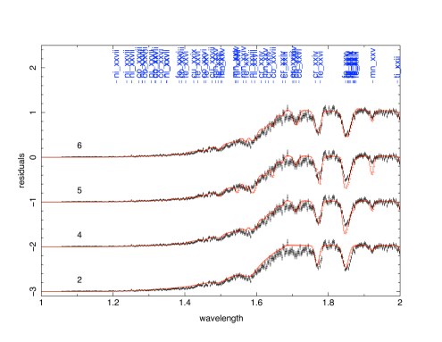
Figure 1: Spectrum $\lambda\lambda$ 1 – 2 Å. Spectrum is shown as ratio relative to pure power law model (model 1). Various models 2,4,5,6 are labeled. The vertical axis is the ratio of the model and data to the continuum-only model, model 1. Successive models are offset by unity from each other.

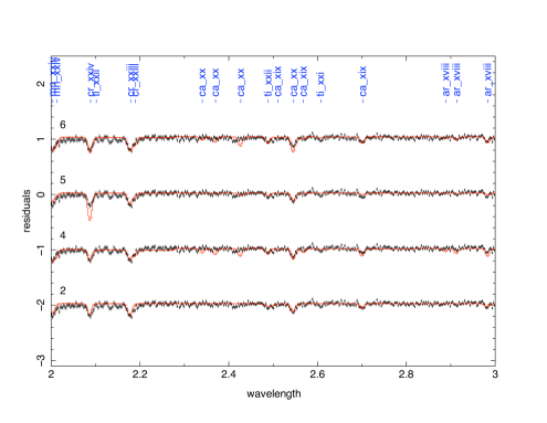
Figure 2: Spectrum $\lambda\lambda$ 2 – 3 Å. Spectrum is shown as ratio relative to pure power law model (model 1). Various models 2,4,5,6 are labeled. The vertical axis is the ratio of the model and data to the continuum-only model, model 1. Successive models are offset by unity from each other.

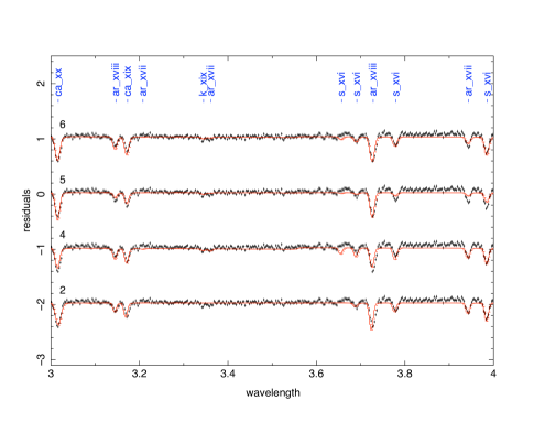
Figure 3: Spectrum $\lambda\lambda$ 3 – 4 Å. Spectrum is shown as ratio relative to pure power law model (model 1). Various models 2,4,5,6 are labeled. The vertical axis is the ratio of the model and data to the continuum-only model, model 1. Successive models are offset by unity from each other.

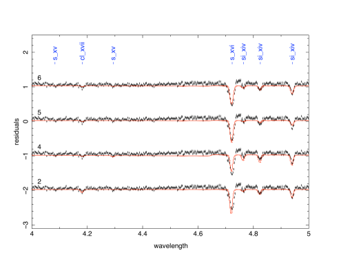
Figure 4: Spectrum $\lambda\lambda$ 4 – 5 Å. Spectrum is shown as ratio relative to pure power law model (model 1). Various models 2,4,5,6 are labeled. The vertical axis is the ratio of the model and data to the continuum-only model, model 1. Successive models are offset by unity from each other.

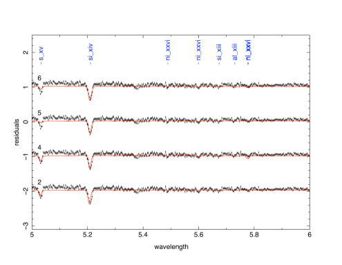
Figure 5: Spectrum $\lambda\lambda$ 5 – 6 Å. Spectrum is shown as ratio relative to pure power law model (model 1). Various models 2,4,5,6 are labeled. The vertical axis is the ratio of the model and data to the continuum-only model, model 1. Successive models are offset by unity from each other.

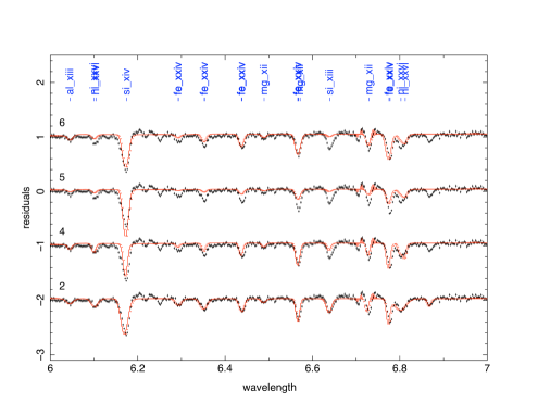
Figure 6: Spectrum $\lambda\lambda$ 6 – 7 Å. Spectrum is shown as ratio relative to pure power law model (model 1). Various models 2,4,5,6 are labeled. The vertical axis is the ratio of the model and data to the continuum-only model, model 1. Successive models are offset by unity from each other.

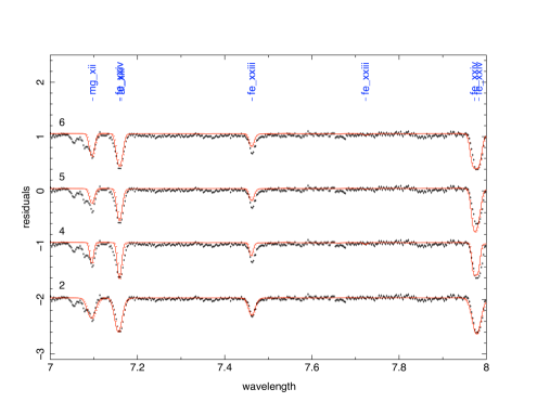
Figure 7: Spectrum $\lambda\lambda$ 7 – 8 Å. Spectrum is shown as ratio relative to pure power law model (model 1). Various models 2,4,5,6 are labeled. The vertical axis is the ratio of the model and data to the continuum-only model, model 1. Successive models are offset by unity from each other.

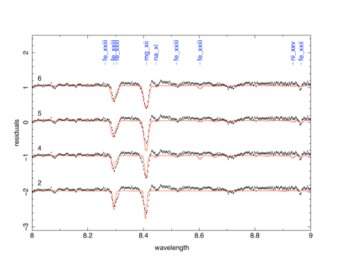
Figure 8: Spectrum $\lambda\lambda$ 8 – 9 Å. Spectrum is shown as ratio relative to pure power law model (model 1). Various models 2,4,5,6 are labeled. The vertical axis is the ratio of the model and data to the continuum-only model, model 1. Successive models are offset by unity from each other.

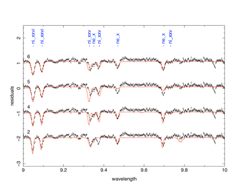
Figure 9: Spectrum $\lambda\lambda$ 9 – 10 Å. Spectrum is shown as ratio relative to pure power law model (model 1). Various models 2,4,5,6 are labeled. The vertical axis is the ratio of the model and data to the continuum-only model, model 1. Successive models are offset by unity from each other.

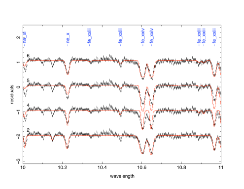
Figure 10: Spectrum $\lambda\lambda$ 10 – 11 Å. Spectrum is shown as ratio relative to pure power law model (model 1). Various models 2,4,5,6 are labeled. The vertical axis is the ratio of the model and data to the continuum-only model, model 1. Successive models are offset by unity from each other.

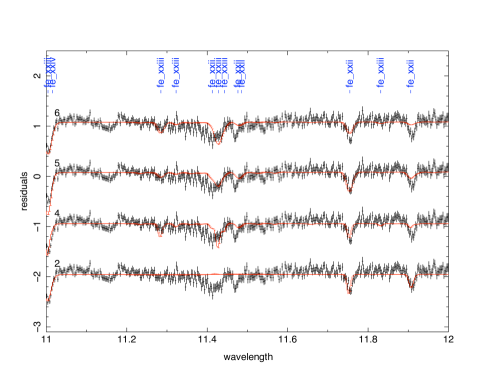
Figure 11: Spectrum $\lambda\lambda$ 11 – 12 Å. Spectrum is shown as ratio relative to pure power law model (model 1). Various models 2,4,5,6 are labeled. The vertical axis is the ratio of the model and data to the continuum-only model, model 1. Successive models are offset by unity from each other.

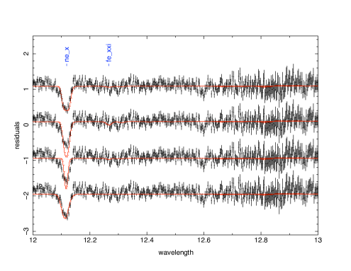
Figure 12: Spectrum $\lambda\lambda$ 12 – 13 Å. Spectrum is shown as ratio relative to pure power law model (model 1). Various models 2,4,5,6 are labeled. The vertical axis is the ratio of the model and data to the continuum-only model, model 1. Successive models are offset by unity from each other.

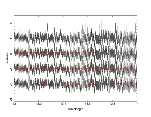
Figure 13: Spectrum $\lambda\lambda$ 13 – 14 Å. Spectrum is shown as ratio relative to pure power law model (model 1). Various models 2,4,5,6 are labeled. The vertical axis is the ratio of the model and data to the continuum-only model, model 1. Successive models are offset by unity from each other.

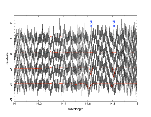
Figure 14: Spectrum $\lambda\lambda$ 14 – 15 Å. Spectrum is shown as ratio relative to pure power law model (model 1). Various models 2,4,5,6 are labeled. The vertical axis is the ratio of the model and data to the continuum-only model, model 1. Successive models are offset by unity from each other.

Table 2: Line Properties

$\lambda_{O}$	index	$\lambda$	ion	v0	ew	width	$\tau$	f	lower level	upper level	ion column
1.544	17264	1.542	Mn XXV	-357.5	0.0006	459.3	0.71${}^{+0.56}_{-0.41}$	0.029	1s.2S	4p.2Po	2.9${}^{+2.3}_{-1.7}\times 10^{23}$
1.567	128239	1.573	Fe XXV	1187.0	0.0029	772.1	2.62${}^{+1.44}_{-0.88}$	0.152	1s2.1S	1s.3p.1P*	4.4${}^{+2.4}_{-1.5}\times 10^{21}$
1.582	132917	1.589	Ni XXVII	1232.6	0.0084	506.7	23.06${}^{+9.99}_{-8.75}$	0.684	1s2.1S	1s.2p.1P	1.0${}^{+0.7}_{-0.4}\times 10^{23}$
1.601			no ID		0.0022	707.2	1.92${}^{+0.91}_{-0.62}$
1.613	17063	1.615	Cr XXIV	297.6	0.0004	234.9	1.18${}^{+0.80}_{-0.60}$	0.008	1s.2S	6p.2Po	1.4${}^{+0.9}_{-0.7}\times 10^{24}$
1.626	17263	1.626	Mn XXV	77.5	0.0010	412.7	1.22${}^{+0.51}_{-0.40}$	0.080	1s.2S	3p.2Po	1.7${}^{+0.7}_{-0.6}\times 10^{23}$
1.646	128543	1.649	Co XXVII	484.8	0.0006	407.0	0.66${}^{+0.34}_{-0.28}$	0.422	1s.2S	2p.2Po	7.4${}^{+3.8}_{-3.1}\times 10^{22}$
1.675	17061	1.674	Cr XXIV	-107.5	0.0004	204.0	1.22${}^{+0.79}_{-0.63}$	0.029	1s.2S	4p.2Po	3.7${}^{+2.4}_{-1.9}\times 10^{23}$
1.693			no ID		0.0007	458.1	0.58${}^{+0.27}_{-0.23}$
1.709	128440	1.712	Co XXVI	544.2	0.0015	539.4	1.24${}^{+0.40}_{-0.31}$	0.693	1s2.1S	1s.2p.1P	8.2${}^{+2.6}_{-2.1}\times 10^{22}$
1.726			no ID		0.0012	701.0	0.65${}^{+0.24}_{-0.22}$
1.742			no ID		0.0003	225.4	0.71${}^{+0.49}_{-0.36}$
1.772	128358	1.780	Fe XXVI	1325.6	0.0053	453.6	10.56${}^{+3.68}_{-2.72}$	0.408	1s.2S	2p.2Po	5.9${}^{+2.1}_{-1.5}\times 10^{21}$
1.838			no ID		0.0007	195.2	2.35${}^{+0.75}_{-0.55}$
1.851	128293	1.850	Fe XXV	-81.0	0.0157	503.9	39.38${}^{+9.99}_{-8.98}$	0.775	1s2.1S	1s.2p.1P*	1.1${}^{+0.3}_{-0.3}\times 10^{22}$
1.865	127741	1.864	Fe XXIV	-209.1	0.0006	179.5	2.57${}^{+0.96}_{-0.70}$	0.149	1s2.2s	1s2s2p.2P0.5	3.7${}^{+1.4}_{-1.0}\times 10^{21}$
1.875	127760	1.873	Fe XXIV	-320.0	0.0003	203.7	0.41${}^{+0.28}_{-0.24}$	0.015	1s2.2s	1s2s2p.4P1.5	5.7${}^{+3.9}_{-3.4}\times 10^{21}$
1.923	17262	1.926	Mn XXV	480.5	0.0007	401.6	0.44${}^{+0.13}_{-0.12}$	0.420	1s.2S	2p.2Po	10.0${}^{+2.9}_{-2.7}\times 10^{21}$
1.951	16659	1.948	Ti XXII	-412.1	0.0002	299.7	0.14${}^{+0.14}_{-0.09}$	0.014	1s.2S	5p.2Po	4.1${}^{+4.0}_{-2.6}\times 10^{23}$
1.963			no ID		0.0003	212.7	0.44${}^{+0.23}_{-0.20}$
1.993	16658	1.995	Ti XXII	313.1	0.0003	207.6	0.36${}^{+0.21}_{-0.19}$	0.029	1s.2S	4p.2Po	5.0${}^{+2.9}_{-2.7}\times 10^{23}$
2.004	17159	2.006	Mn XXIV	329.4	0.0018	566.0	0.87${}^{+0.15}_{-0.14}$	0.711	1s2.1S	1s.2p.1P	1.1${}^{+0.2}_{-0.2}\times 10^{22}$
2.020			no ID		0.0007	493.5	0.32${}^{+0.10}_{-0.09}$
2.036			no ID		0.0003	454.9	0.17${}^{+0.09}_{-0.09}$
2.062			no ID		0.0003	442.3	0.14${}^{+0.08}_{-0.08}$
2.088	17059	2.092	Cr XXIV	502.9	0.0014	416.2	0.84${}^{+0.13}_{-0.12}$	0.421	1s.2S	2p.2Po	1.4${}^{+0.2}_{-0.2}\times 10^{22}$
2.114			no ID		0.0002	161.4	0.26${}^{+0.20}_{-0.17}$
2.153			no ID		0.0005	156.3	0.73${}^{+0.28}_{-0.26}$
2.179	16956	2.182	Cr XXIII	426.8	0.0020	526.2	0.87${}^{+0.11}_{-0.11}$	0.721	1s2.1S	1s.2p.1P	8.2${}^{+1.0}_{-1.0}\times 10^{21}$
2.193	17016	2.193	Cr XXIII	-68.4	0.0004	181.7	0.52${}^{+0.20}_{-0.18}$	0.152	1s2.1S	1s.2p.3P	2.3${}^{+0.9}_{-0.8}\times 10^{22}$
2.205			no ID		0.0002	158.5	0.22${}^{+0.20}_{-0.14}$
2.312			no ID		0.0003	158.4	0.27${}^{+0.19}_{-0.17}$
2.361			no ID		0.0003	396.3	0.10${}^{+0.06}_{-0.05}$
2.417			no ID		0.0004	403.5	0.15${}^{+0.06}_{-0.05}$
2.491	16656	2.492	Ti XXII	150.5	0.0007	410.0	0.22${}^{+0.05}_{-0.05}$	0.419	1s.2S	2p.2Po	1.7${}^{+0.4}_{-0.4}\times 10^{22}$
2.502	16183	2.514	Ca XIX	1414.8	0.0003	151.4	0.30${}^{+0.16}_{-0.14}$	0.027	1s2.1S	1s.5p.1P*	2.5${}^{+1.3}_{-1.2}\times 10^{22}$
2.545	16282	2.549	Ca XX	515.1	0.0011	136.9	1.69${}^{+0.29}_{-0.26}$	0.078	1s.2S	3p.2Po	4.8${}^{+0.8}_{-0.7}\times 10^{22}$
2.555			no ID		0.0002	140.0	0.20${}^{+0.17}_{-0.13}$
2.701	16143	2.705	Ca XIX	488.7	0.0008	400.9	0.21${}^{+0.05}_{-0.05}$	0.152	1s2.1S	1s.3p.1P*	2.9${}^{+0.7}_{-0.7}\times 10^{21}$
2.857			no ID		0.0003	117.3	0.18${}^{+0.13}_{-0.11}$
2.877			no ID		0.0003	124.1	0.23${}^{+0.16}_{-0.15}$
2.982	13532	2.987	Ar XVIII	548.3	0.0007	131.4	0.48${}^{+0.15}_{-0.13}$	0.029	1s.2S	4p.2Po	1.5${}^{+0.5}_{-0.4}\times 10^{22}$
3.016	16262	3.020	Ca XX	427.7	0.0050	415.2	1.24${}^{+0.08}_{-0.07}$	0.411	1s.2S	2p.2Po	5.7${}^{+0.4}_{-0.3}\times 10^{21}$
3.145	13528	3.151	Ar XVIII	534.2	0.0016	304.3	0.40${}^{+0.06}_{-0.05}$	0.078	1s.2S	3p.2Po	4.3${}^{+0.6}_{-0.6}\times 10^{21}$
3.172	16146	3.177	Ca XIX	491.8	0.0024	203.9	1.08${}^{+0.12}_{-0.12}$	0.770	1s2.1S	1s.2p.1P*	2.5${}^{+0.3}_{-0.3}\times 10^{21}$
3.355	13463	3.365	Ar XVII	938.9	0.0009	476.4	0.11${}^{+0.03}_{-0.03}$	0.153	1s2.1S	1s.3p.1P*	5.5${}^{+1.8}_{-1.7}\times 10^{20}$
3.690	11876	3.696	S XVI	479.7	0.0012	107.1	0.49${}^{+0.14}_{-0.15}$	0.014	1s.2S	5p.2Po	8.0${}^{+2.4}_{-2.4}\times 10^{21}$
3.727	13535	3.733	Ar XVIII	474.9	0.0072	351.1	1.08${}^{+0.07}_{-0.06}$	0.412	1s.2S	2p.2Po	1.9${}^{+0.1}_{-0.1}\times 10^{21}$
3.779	11875	3.784	S XVI	429.5	0.0019	86.5	1.18${}^{+0.30}_{-0.24}$	0.029	1s.2S	4p.2Po	9.0${}^{+2.3}_{-1.8}\times 10^{21}$
3.943	13446	3.949	Ar XVII	441.3	0.0025	85.2	1.70${}^{+0.33}_{-0.28}$	0.766	1s2.1S	1s.2p.1P*	1.5${}^{+0.3}_{-0.2}\times 10^{21}$
3.985	11878	3.991	S XVI	466.8	0.0044	173.4	1.20${}^{+0.14}_{-0.12}$	0.079	1s.2S	3p.2Po	3.2${}^{+0.4}_{-0.3}\times 10^{21}$
4.183	12039	4.188	Cl XVII	329.9	0.0012	90.5	0.41${}^{+0.16}_{-0.15}$	0.416	1s.2S	2p.2Po	7.4${}^{+3.0}_{-2.7}\times 10^{21}$
4.722	11871	4.729	S XVI	457.4	0.0184	407.6	1.27${}^{+0.08}_{-0.07}$	0.413	1s.2S	2p.2Po	5.4${}^{+0.3}_{-0.3}\times 10^{20}$
4.764	9813	4.770	Si XIV	403.0	0.0008	72.9	0.20${}^{+0.22}_{-0.12}$	0.008	1s.2S	6p.2Po	2.2${}^{+2.4}_{-1.4}\times 10^{21}$
4.824	9810	4.831	Si XIV	441.5	0.0031	128.4	0.48${}^{+0.14}_{-0.13}$	0.014	1s.2S	5p.2Po	2.9${}^{+0.9}_{-0.8}\times 10^{21}$
4.941	9811	4.947	Si XIV	358.2	0.0053	86.8	1.98${}^{+0.51}_{-0.37}$	0.029	1s.2S	4p.2Po	5.6${}^{+1.4}_{-1.1}\times 10^{21}$
5.032	11734	5.039	S XV	401.2	0.0044	66.2	2.07${}^{+0.46}_{-0.37}$	0.761	1s2.1S	1s.2p.1P*	4.5${}^{+1.0}_{-0.8}\times 10^{20}$
5.209	9817	5.217	Si XIV	472.2	0.0115	237.9	0.92${}^{+0.09}_{-0.08}$	0.079	1s.2S	3p.2Po	9.1${}^{+0.9}_{-0.8}\times 10^{20}$
5.375			no ID		0.0022	244.9	0.11${}^{+0.05}_{-0.05}$
5.600	132830	5.606	Ni XXVI	332.2	0.0023	62.5	0.46${}^{+0.22}_{-0.20}$	0.007	1s2.2s	1S2_7p	6.2${}^{+2.9}_{-2.7}\times 10^{22}$
6.004			no ID		0.0010	78.3	0.12${}^{+0.09}_{-0.07}$
6.018			no ID		0.0025	64.8	0.37${}^{+0.13}_{-0.13}$
6.045	8043	6.053	Al XIII	392.0	0.0063	414.3	0.14${}^{+0.02}_{-0.02}$	0.079	1s.2S	3p.2Po	1.8${}^{+0.3}_{-0.3}\times 10^{21}$
6.065			no ID		0.0014	55.7	0.23${}^{+0.14}_{-0.13}$
6.077			no ID		0.0031	50.3	0.66${}^{+0.23}_{-0.21}$
6.103	132826	6.108	Ni XXVI	226.1	0.0088	407.7	0.22${}^{+0.02}_{-0.02}$	0.024	1s2.2s	1s2.5p	7.4${}^{+0.8}_{-0.7}\times 10^{21}$
6.135			no ID		0.0020	62.9	0.28${}^{+0.12}_{-0.12}$
6.154	9816	6.182	Si XIV	1374.7	0.0034	164.6	0.17${}^{+0.04}_{-0.04}$	0.414	1s.2S	2p.2Po	2.7${}^{+0.7}_{-0.6}\times 10^{19}$
6.172	9816	6.182	Si XIV	495.8	0.0414	419.4	1.35${}^{+0.04}_{-0.04}$	0.414	1s.2S	2p.2Po	2.1${}^{+0.1}_{-0.1}\times 10^{20}$
6.295			no ID		0.0075	332.6	0.20${}^{+0.03}_{-0.02}$
6.352	128163	6.360	Fe XXIV	392.0	0.0138	425.8	0.28${}^{+0.02}_{-0.02}$	0.002	1s2.2s	1S2_9p	7.8${}^{+0.6}_{-0.6}\times 10^{21}$
6.375			no ID		0.0025	58.5	0.35${}^{+0.13}_{-0.13}$
6.413			no ID		0.0020	58.8	0.27${}^{+0.13}_{-0.12}$
6.440	128161	6.446	Fe XXIV	270.2	0.0139	274.1	0.41${}^{+0.03}_{-0.03}$	0.004	1s2.2s	1S2_8p	6.5${}^{+0.5}_{-0.5}\times 10^{21}$
6.489	7856	6.497	Mg XII	389.7	0.0043	162.7	0.19${}^{+0.04}_{-0.04}$	0.008	1s.2S	6p.2Po	1.7${}^{+0.4}_{-0.4}\times 10^{21}$
6.550			no ID		0.0019	67.4	0.20${}^{+0.10}_{-0.10}$
6.569	128159	6.575	Fe XXIV	260.3	0.0204	242.7	0.74${}^{+0.04}_{-0.04}$	0.007	1s2.2s	1S2_7p	6.7${}^{+0.3}_{-0.4}\times 10^{21}$
6.590	7853	6.580	Mg XII	-455.2	0.0013	59.5	0.15${}^{+0.11}_{-0.09}$	0.014	1s.2S	5p.2Po	6.9${}^{+5.4}_{-4.4}\times 10^{20}$
6.640	9691	6.648	Si XIII	361.4	0.0163	291.7	0.42${}^{+0.03}_{-0.03}$	0.748	1s2.1S	1s.2p.1P*	3.4${}^{+0.3}_{-0.3}\times 10^{19}$
6.729	7852	6.738	Mg XII	401.2	0.0100	54.7	3.40${}^{+0.92}_{-0.59}$	0.029	1s.2S	4p.2Po	7.7${}^{+2.1}_{-1.3}\times 10^{21}$
6.778	128157	6.784	Fe XXIV	256.7	0.0269	289.2	0.76${}^{+0.03}_{-0.03}$	0.012	1s2.2s	1S2_6p	3.7${}^{+0.2}_{-0.1}\times 10^{21}$
6.805	132821	6.811	Ni XXVI	264.5	0.0198	416.0	0.34${}^{+0.02}_{-0.02}$	0.032	1s2.2s	1s2.4p	7.7${}^{+0.5}_{-0.4}\times 10^{21}$
6.842			no ID		0.0013	75.2	0.11${}^{+0.07}_{-0.07}$
6.869			no ID		0.0090	271.0	0.20${}^{+0.03}_{-0.02}$
6.956			no ID		0.0015	73.4	0.12${}^{+0.08}_{-0.07}$
7.013			no ID		0.0026	58.3	0.26${}^{+0.10}_{-0.10}$
7.058			no ID		0.0144	445.5	0.20${}^{+0.02}_{-0.02}$
7.093	7855	7.106	Mg XII	557.0	0.0426	495.7	0.61${}^{+0.02}_{-0.02}$	0.079	1s.2S	3p.2Po	4.8${}^{+0.2}_{-0.2}\times 10^{20}$
7.159	128021	7.169	Fe XXIV	419.1	0.0556	392.7	1.17${}^{+0.02}_{-0.02}$	0.026	1s2.2s	1s2.5p	2.5${}^{+0.1}_{-0.1}\times 10^{21}$
7.223			no ID		0.0022	48.2	0.25${}^{+0.12}_{-0.11}$
7.242			no ID		0.0058	312.1	0.11${}^{+0.01}_{-0.04}$
7.265			no ID		0.0024	68.3	0.18${}^{+0.07}_{-0.06}$
7.283			no ID		0.0030	60.1	0.27${}^{+0.08}_{-0.08}$
7.373			no ID		0.0051	47.7	0.64${}^{+0.14}_{-0.13}$
7.387			no ID		0.0029	65.1	0.22${}^{+0.07}_{-0.07}$
7.400			no ID		0.0020	61.6	0.15${}^{+0.07}_{-0.07}$
7.415			no ID		0.0029	61.9	0.23${}^{+0.08}_{-0.07}$
7.432			no ID		0.0026	54.2	0.24${}^{+0.09}_{-0.09}$
7.464	126341	7.472	Fe XXIII	321.5	0.0272	348.1	0.48${}^{+0.02}_{-0.02}$	0.056	2s2	2s.5p	4.7${}^{+0.2}_{-0.2}\times 10^{20}$
7.490			no ID		0.0036	58.0	0.31${}^{+0.09}_{-0.09}$
7.513			no ID		0.0023	52.0	0.21${}^{+0.11}_{-0.11}$
7.533			no ID		0.0034	59.9	0.27${}^{+0.10}_{-0.09}$
7.555			no ID		0.0020	59.7	0.15${}^{+0.08}_{-0.08}$
7.575			no ID		0.0042	53.8	0.38${}^{+0.11}_{-0.10}$
7.617			no ID		0.0022	43.5	0.23${}^{+0.15}_{-0.14}$
7.664			no ID		0.0067	278.2	0.10${}^{+0.03}_{-0.02}$
7.700	126899	7.733	Fe XXIII	1285.7	0.0027	48.3	0.25${}^{+0.12}_{-0.11}$	0.035	2s.2p	2s.5d	3.6${}^{+1.8}_{-1.7}\times 10^{20}$
7.722	126899	7.733	Fe XXIII	427.3	0.0018	46.4	0.17${}^{+0.12}_{-0.11}$	0.035	2s.2p	2s.5d	2.5${}^{+1.8}_{-1.6}\times 10^{20}$
7.743	126899	7.733	Fe XXIII	-387.5	0.0030	72.0	0.18${}^{+0.07}_{-0.06}$	0.035	2s.2p	2s.5d	2.6${}^{+1.0}_{-0.9}\times 10^{20}$
7.850			no ID		0.0056	48.5	0.55${}^{+0.13}_{-0.13}$
7.863			no ID		0.0037	53.6	0.29${}^{+0.10}_{-0.10}$
7.875			no ID		0.0037	57.2	0.27${}^{+0.09}_{-0.09}$
7.890			no ID		0.0028	51.8	0.22${}^{+0.10}_{-0.10}$
7.904			no ID		0.0035	59.5	0.24${}^{+0.09}_{-0.08}$
7.946	127946	7.983	Fe XXIV	1396.9	0.0019	51.1	0.14${}^{+0.09}_{-0.08}$	0.062	1s2.2s	1s2.4p	1.2${}^{+0.7}_{-0.6}\times 10^{20}$
7.980	127946	7.983	Fe XXIV	112.8	0.0829	409.0	1.24${}^{+0.04}_{-0.02}$	0.062	1s2.2s	1s2.4p	1.0${}^{+0.0}_{-0.0}\times 10^{21}$
8.081	120327	8.090	Fe XXII	348.9	0.0043	52.5	0.33${}^{+0.10}_{-0.09}$	0.050	2s2.2p	2s2.5d	3.3${}^{+1.0}_{-0.9}\times 10^{20}$
8.296	125709	8.303	Fe XXIII	249.5	0.0431	311.2	0.67${}^{+0.03}_{-0.03}$	0.144	2s2	2s.4p	2.3${}^{+0.1}_{-0.1}\times 10^{20}$
8.393	7883	8.421	Mg XII	1000.8	0.0042	50.3	0.29${}^{+0.12}_{-0.11}$	0.414	1s.2S	2p.2Po	3.6${}^{+1.5}_{-1.4}\times 10^{19}$
8.409	7883	8.421	Mg XII	428.1	0.0704	285.7	1.28${}^{+0.04}_{-0.04}$	0.414	1s.2S	2p.2Po	1.6${}^{+0.0}_{-0.0}\times 10^{20}$
8.705	119538	8.715	Fe XXII	344.6	0.0061	54.4	0.36${}^{+0.11}_{-0.11}$	0.062	2s2.2p	2s.2p(3P).4p	2.7${}^{+0.8}_{-0.8}\times 10^{20}$
8.721	119538	8.715	Fe XXII	-206.4	0.0057	57.7	0.31${}^{+0.10}_{-0.10}$	0.062	2s2.2p	2s.2p(3P).4p	2.3${}^{+0.8}_{-0.7}\times 10^{20}$
8.963	119527	8.977	Fe XXII	478.6	0.0077	41.5	0.61${}^{+0.19}_{-0.18}$	0.122	2s2.2p	2s2.4d	2.2${}^{+0.7}_{-0.6}\times 10^{20}$
9.048	132824	9.061	Ni XXVI	431.0	0.0602	244.6	0.88${}^{+0.05}_{-0.04}$	0.248	1s2.2s	1s2.3p	1.9${}^{+0.1}_{-0.1}\times 10^{21}$
9.092	132807	9.105	Ni XXVI	428.9	0.0409	180.2	0.76${}^{+0.06}_{-0.05}$	0.130	1s2.2s	1s2.3p	3.2${}^{+0.2}_{-0.2}\times 10^{21}$
9.158	7744	9.169	Mg XI	353.8	0.0038	36.1	0.28${}^{+0.21}_{-0.18}$	0.738	1s2.1S	1s.2p.1P	1.8${}^{+1.3}_{-1.1}\times 10^{19}$
9.336	132741	9.340	Ni XXV	118.9	0.0414	304.6	0.42${}^{+0.03}_{-0.03}$	0.462	2s2	2s.3p	4.7${}^{+0.3}_{-0.4}\times 10^{20}$
9.373	132694	9.390	Ni XXV	534.5	0.0289	164.9	0.48${}^{+0.05}_{-0.05}$	0.231	2s2	2s.3p	1.1${}^{+0.1}_{-0.1}\times 10^{21}$
9.469	6241	9.481	Ne X	380.2	0.0299	181.8	0.42${}^{+0.04}_{-0.04}$	0.014	1s.2S	5p.2Po	1.9${}^{+0.2}_{-0.2}\times 10^{21}$
9.695	6218	9.708	Ne X	402.3	0.0403	189.3	0.54${}^{+0.05}_{-0.05}$	0.029	1s.2S	4p.2Po	1.1${}^{+0.1}_{-0.1}\times 10^{21}$
9.723	6218	9.708	Ne X	-462.8	0.0039	58.1	0.14${}^{+0.12}_{-0.09}$	0.029	1s.2S	4p.2Po	3.0${}^{+2.5}_{-1.9}\times 10^{20}$
9.783			no ID		0.0037	40.3	0.19${}^{+0.18}_{-0.12}$
10.010	6380	10.021	Na XI	323.7	0.0531	183.2	0.72${}^{+0.07}_{-0.06}$	0.416	1s.2S	2p.2Po	9.6${}^{+0.9}_{-0.8}\times 10^{20}$
10.100			no ID		0.0122	59.5	0.43${}^{+0.16}_{-0.14}$
10.150			no ID		0.0234	88.0	0.60${}^{+0.12}_{-0.11}$
10.210	6207	10.240	Ne X	881.5	0.0047	48.1	0.18${}^{+0.16}_{-0.11}$	0.079	1s.2S	3p.2Po	1.3${}^{+1.2}_{-0.8}\times 10^{20}$
10.220	6207	10.240	Ne X	587.1	0.0879	250.4	0.87${}^{+0.05}_{-0.05}$	0.079	1s.2S	3p.2Po	6.5${}^{+0.4}_{-0.4}\times 10^{20}$
10.340	124604	10.349	Fe XXIII	255.3	0.0086	57.1	0.28${}^{+0.16}_{-0.14}$	0.006	2s2	2p.3d	1.8${}^{+1.1}_{-0.9}\times 10^{21}$
10.490	124935	10.505	Fe XXIII	443.3	0.0233	66.5	0.77${}^{+0.21}_{-0.16}$	0.021	2s2	2p.3s	1.4${}^{+0.4}_{-0.3}\times 10^{21}$
10.570	127980	10.619	Fe XXIV	1390.7	0.0309	479.7	0.12${}^{+0.03}_{-0.03}$	0.247	1s2.2s	1s2.3p	1.8${}^{+0.5}_{-0.5}\times 10^{19}$
10.610	127980	10.619	Fe XXIV	254.5	0.2323	490.0	1.30${}^{+0.05}_{-0.06}$	0.247	1s2.2s	1s2.3p	2.0${}^{+0.1}_{-0.1}\times 10^{20}$
10.650	127947	10.663	Fe XXIV	366.2	0.3370	716.3	1.13${}^{+0.05}_{-0.05}$	0.129	1s2.2s	1s2.3p	3.3${}^{+0.1}_{-0.2}\times 10^{20}$
10.780	124988	10.785	Fe XXIII	128.0	0.0346	478.1	0.12${}^{+0.04}_{-0.03}$	0.002	2s2	2s.3d	2.5${}^{+0.7}_{-0.7}\times 10^{21}$
10.890	124606	10.903	Fe XXIII	352.6	0.0402	435.8	0.15${}^{+0.04}_{-0.03}$	0.082	2s.2p	2p.3p	6.8${}^{+1.6}_{-1.5}\times 10^{19}$
10.930	125174	10.980	Fe XXIII	1372.3	0.0079	41.0	0.31${}^{+0.25}_{-0.19}$	0.414	2s2	2s.3p	2.7${}^{+2.2}_{-1.7}\times 10^{19}$
10.970	125174	10.980	Fe XXIII	273.5	0.1490	406.7	0.74${}^{+0.05}_{-0.04}$	0.414	2s2	2s.3p	6.6${}^{+0.4}_{-0.4}\times 10^{19}$
11.010	125372	11.018	Fe XXIII	218.0	0.1051	221.2	0.99${}^{+0.07}_{-0.08}$	0.254	2s2	2s.3p	1.4${}^{+0.1}_{-0.1}\times 10^{20}$
11.150			no ID		0.0350	382.1	0.15${}^{+0.04}_{-0.04}$
11.280	125155	11.299	Fe XXIII	508.0	0.0289	253.5	0.15${}^{+0.06}_{-0.06}$	0.751	2s.2p	2s.3d	7.3${}^{+2.8}_{-2.8}\times 10^{18}$
11.310	125155	11.299	Fe XXIII	-289.1	0.0224	170.2	0.18${}^{+0.08}_{-0.08}$	0.751	2s.2p	2s.3d	8.5${}^{+4.0}_{-3.9}\times 10^{18}$
11.350	124975	11.337	Fe XXIII	-348.9	0.0504	481.3	0.16${}^{+0.06}_{-0.05}$	0.552	2s.2p	2s.3d	1.0${}^{+0.4}_{-0.3}\times 10^{19}$
11.420	124980	11.442	Fe XXIII	585.8	0.1575	500.7	0.52${}^{+0.08}_{-0.07}$	0.615	2s.2p	2s.3d	3.0${}^{+0.4}_{-0.4}\times 10^{19}$
11.470	124991	11.457	Fe XXIII	-337.4	0.0621	253.4	0.34${}^{+0.08}_{-0.07}$	0.110	2s.2p	2s.3d	1.1${}^{+0.3}_{-0.2}\times 10^{20}$
11.540			no ID		0.0357	437.0	0.11${}^{+0.04}_{-0.04}$
11.760	119502	11.769	Fe XXII	242.3	0.0710	192.6	0.51${}^{+0.09}_{-0.08}$	0.673	2s2.2p	2s2.3d	2.6${}^{+0.5}_{-0.4}\times 10^{19}$
11.910	120311	11.921	Fe XXII	277.1	0.0546	145.6	0.50${}^{+0.12}_{-0.11}$	0.597	2s2.2p	2s2.3d	2.9${}^{+0.7}_{-0.6}\times 10^{19}$
12.120	6204	12.134	Ne X	344.1	0.2336	358.4	1.09${}^{+0.08}_{-0.08}$	0.415	1s.2S	2p.2Po	1.3${}^{+0.1}_{-0.1}\times 10^{20}$
12.300	89984	12.282	Fe XXI	-431.7	0.0226	66.1	0.40${}^{+0.26}_{-0.21}$	1.305	2s2.2p2	2s2.2p.3d	10.0${}^{+6.6}_{-5.2}\times 10^{18}$
12.600			no ID		0.0550	163.0	0.36${}^{+0.12}_{-0.11}$
12.640			no ID		0.0319	208.2	0.15${}^{+0.09}_{-0.09}$
12.820			no ID		0.0703	500.8	0.15${}^{+0.12}_{-0.09}$
12.870			no ID		0.0566	213.6	0.25${}^{+0.20}_{-0.16}$
13.110			no ID		0.0700	175.5	0.38${}^{+0.19}_{-0.17}$
13.240			no ID		0.0744	300.9	0.21${}^{+0.14}_{-0.12}$
13.310			no ID		0.0464	118.2	0.35${}^{+0.29}_{-0.22}$
13.450			no ID		0.2285	553.4	0.41${}^{+0.13}_{-0.11}$
13.540			no ID		0.1563	564.8	0.25${}^{+0.12}_{-0.11}$
13.580			no ID		0.0313	30.1	1.27${}^{+9.99}_{-0.80}$
13.660			no ID		0.0443	29.2	3.28${}^{+9.99}_{-2.07}$
13.680			no ID		0.0365	26.1	2.42${}^{+9.99}_{-1.52}$
13.770			no ID		0.1267	268.8	0.39${}^{+0.19}_{-0.17}$
13.820			no ID		0.0393	29.6	1.92${}^{+9.99}_{-1.21}$
13.880			no ID		0.1279	450.4	0.24${}^{+0.13}_{-0.12}$
13.930			no ID		0.0883	150.1	0.49${}^{+0.29}_{-0.23}$
14.010			no ID		0.1935	482.0	0.35${}^{+0.14}_{-0.13}$
14.090	16073	14.097	Ca XVIII	149.0	0.1243	302.6	0.40${}^{+0.17}_{-0.15}$	0.062	1s2.2s	1s2.4p	2.6${}^{+1.1}_{-1.0}\times 10^{21}$
14.160			no ID		0.0626	72.3	0.77${}^{+0.73}_{-0.49}$
14.190			no ID		0.1305	246.3	0.40${}^{+0.21}_{-0.18}$
14.250			no ID		0.0399	27.8	1.85${}^{+9.99}_{-1.17}$
14.300			no ID		0.1415	160.0	0.77${}^{+0.34}_{-0.27}$
14.360			no ID		0.0404	27.8	1.81${}^{+9.99}_{-1.14}$
14.390			no ID		0.1554	266.4	0.43${}^{+0.19}_{-0.17}$
14.430			no ID		0.0576	78.8	0.56${}^{+0.59}_{-0.36}$
14.470			no ID		0.0527	112.3	0.32${}^{+0.38}_{-0.20}$
14.550			no ID		0.0577	26.3	7.71${}^{+9.99}_{-4.86}$
14.610	4675	14.645	O VIII	724.9	0.1763	189.3	0.75${}^{+0.30}_{-0.25}$	0.008	1s.2S	6p.2Po	1.8${}^{+0.7}_{-0.6}\times 10^{20}$
14.770	4634	14.832	O VIII	1255.2	0.0501	26.7	3.02${}^{+9.99}_{-1.90}$	0.014	1s.2S	5p.2Po	4.1${}^{+9.9}_{-2.6}\times 10^{20}$
14.820	4634	14.832	O VIII	238.9	0.1715	454.9	0.26${}^{+0.15}_{-0.13}$	0.014	1s.2S	5p.2Po	3.5${}^{+2.0}_{-1.8}\times 10^{19}$

The range between 1-2.5 Å is dominated by the H-like L$\alpha$ and He-like allowed $n=$1 – 2 lines from the elements Fe (1.77, 1.85 Å ), Mn (1.92, 2.01 Å ) and Cr (2.08, 2.18 Å ). Wavelengths shortward of the Fe XXVI L$\alpha$ line at 1.77 Å contain the K lines of elements heavier than Fe, in addition to the higher series lines of Fe. Although there are marginal detections of some of these lines, there are too few counts in this region to strongly constrain the abundances of the heavier elements Co, Cu, Zn. Ni is an exception to this, since it also has lines from Li-like Ni XXVI at longer wavelength. It is important to emphasize that, although Ly$\alpha$ lines are not clearly detected for Co, Cu and Zn, we cannot set meaningful upper limits to their strength because our model atoms for these elements do not include $n=$2 – 3 lines from the Li-like and lower ionization stages.

The 2 – 3 Å region includes the He-like resonance line of Mn XXIV, the K lines from H- and He-like Cr (2.088 and 2.179 Å ), He-like Sc (2.877 Å ), H-like Ti (2.491 Å ). The apparent absence of lines from V, H-like Sc and He-like Ti provides relatively secure upper limits on the abundances of these elements. We point out that the existence of evaluated wavelengths for these lines from NIST provides added validity to this conclusion. In this range are also $n=$1 – 3 lines from Ca, which are stronger than the $n=$1 – 2 lines from Sc, Ti, Cr and Mn. In this range are also $n=$1 – 3 lines from Ca, Ar, S, Si. For Si XIV Rydberg series lines are detected up to $n=6$.

At 4.18 Å we marginally detect the L$\alpha$ line from H-like Cl XVII. The He-like line from this element is not detected, but we note the absence of evaluated wavelength for this line. Similar comments apply to the H-like line from P, near 5.38 Å. The ratio of the He and H-like lines from S near 4.72 and 5.04 Å follows the same behavior as for Ca and Ar. The 6 –7Å region is dominated by lines from Si XIII and XIV and Li-like Fe and Ni; for Fe these are detected up to $1s^{2}2s-1s^{2}10p$. At 10.67 and 10.88Å are the lines from Fe XXII which provide the density diagnostics. These lines together extend the range of ionization of observed species to include ions which are indicative of lower ionization parameter gas than the hydrogenic and helium-like ions which predominate.

Table 2 includes 175 lines of which 100 have IDs. The table of Miller et al. (2008) includes 102 lines, of which 15 have no IDs. Our table has 44 lines which are not in the Miller et al. (2008) table, although we note that they used a 5$\sigma$ criterion for line detection, while ours is 3$\sigma$. Of the unidentified lines in Miller et al. (2008) we propose IDs for 5.6 Å Ni XXVI 2s – 7p and 9.372 Å Ni XXV 2s² – 2s3p. We have no IDs for the unidentified lines from Miller et al. (2008) at $\lambda\lambda$ 6.25, 7.0555, 7.0851, 9.9509 Å. These latter 3 are crudely consistent with lines arising from the 2p excited levels of Ni XXVI (rest wavelengths 7.048, 7.0950 and 9.6383). But the results of warmabs suggest optical depths for these lines which are smaller than the resonance lines by factors $\geq 10^{4}$ assuming a density of 10¹⁵ cm^-3 and no trapping of line radiation. All the 75 lines from our notch model for which we have no identifications, have small equivalent widths, within a factor of 2 of our cutoff of 3.5 $\times 10^{-4}$. We speculate that some of them could be due to the notch algorithm attempting to correct for discrepancies between the model continuum and the data, perhaps due to bound-free continuum absorption. In addition, visual inspection of the spectrum shows lines which do not appear in our table. Many of these have possible IDs as lines from excited levels, but none appears in the warmabs models at sufficient strength to be included in our table. Other lines in this category include: 2.60 Å possibly Ti XXI He-like 1 – 2, 2.15 Å possibly Sc XX He-like 1 – 3, features at 3.61, 5.375, 5.62, 5.65 Å with no obvious ID, and 5.72 Å possibly Al XIII 1 – 4. Features at 6.22 and 6.24 Å could be due to Si XIII 1s2s – 2s2p. Discernible features at $\lambda\lambda$ 6.7, 6.87, 7.06, 9.24, 9.78, 9.96, 10.1, 10.15 and 11.15 Å  have no obvious IDs. Many of these correspond to lines in our list which are from excited levels, or from ion stages which are too low to coexist with the dominant ions in the warmabs models. We also note an emission line at 13.38 Å which coincides with the $\lambda$ 13.387 Å 2s – 3p transition in Ti XXII listed in Shirai et al. (2000). If this is correct, it is hard understand why this line should appear in emission when other analogous lines from Fe XXIV and Ni XXVI, for instance, appear in absorption. Other interesting lines not identified by Miller et al. (2008) are the Fe XXIII lines between 11.28 Å and 11.47 Å, since they arise from the metastable 2s2p${}^{3}P$ level. Their presence corroborates the density estimate from the Fe XXII lines.

The Doppler shift of the lines relative to the lab wavelength are shown graphically in figure 15. In this figure, the color corresponds to the element, and the size of the dot corresponds to the line optical depth. This shows that the lines cluster in a range around 400 km s^-1 from zero offset (here and in what follows we quote blueshifted velocities as positive, and conversely). This corresponds to $\sim$2 – 10 mÅ for most lines. Many of the laboratory wavelengths are uncertain at this level. Given this, the most notable aspect of the line shifts is the large velocity offset of the Fe XXVI L$\alpha$ and the Ni XXVII lines. These are among the strongest lines in the spectrum, and are blueshifted by $\simeq$1300 km/s, which is significantly greater than any other lines in the spectrum. This, together with the fact that these are the two highest-ionization lines in the spectrum, suggests that these lines are partly formed in a separate component of the flow. If so, this component would have higher ionization, and higher velocity, than the component responsible for the rest of the lines. On the other hand, we consider the possibility that this is an artifact of shortcomings in the HETG calibration when applied to fitting absorption of the steeply sloping continuum under these lines. In what follows we will examine alternative explanations for this in our fits to the spectrum.

The line widths in Table 2 range from 1 – 10 mÅ. We have searched and found no significant correlation between this quantity and simple quantities characterizing the parent ion, such as the ionization potential or isoelectronic sequence. There is a weak tendency for the largest widths to be associated with lower ionization potential ions. An example is the L$\alpha$ line from Si XIV. However, there are also narrower lines from ions with comparable ionization potential, so this does not constitute a statistically significant correlation.

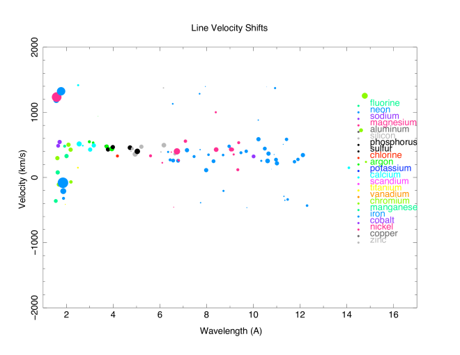
Figure 15: Doppler velocities obtained by comparing measured notch wavelengths with lab wavelengths from xstar database. Element color coding is given in the legend. The dot size is proportional to the line optical depth.

2.2 Ion Column Densities

Ion column densities can be derived from the line identifications in Table 2, assuming that the equivalent widths lie on the linear part of the curve of growth. That is, we calculate

$$N_{ion}=\frac{\tau_{line}}{\frac{\pi e^{2}}{m_{e}c}\frac{f}{\Delta\nu_{D}}}$$ (1)

where $\Delta\nu_{D}$ is the total Doppler width in frequency units, including both thermal and turbulent contributions. $\tau_{line}$ is the line depth measured from the notch fit to the spectrum, and since it is based on Gaussian line fits its accuracy diminishes when values become large. In Table 2 we list the value of the ratio $N_{ion}/Y_{element}$, where $Y_{element}$ is the elemental solar (Grevesse et al., 1996; Allen, 1973) abundance relative to hydrogen. $N_{ion}/Y_{element}$, is the equivalent hydrogen column density implied by a given line if its ion fraction were unity, if the elemental abundance were solar, and if it lies on the linear part of the curve of growth. In figure 16 we plot this quantity. The horizontal axis is related to the atomic number of the parent element by $Z_{ion}=Z_{element}+1-0.1*(ionstage)$, where $(ionstage)$=1 for hydrogenic, 2 for He-like, etc. Error bars are plotted and, in most cases, are small compared with the the interval between points. If the assumptions of unit ionization fraction, cosmic abundances, and linear curve of growth were correct, then all the points in this diagram would lie along one horizontal line. Since most elements have lines from more than one ion, the assumption of unit ionization fraction cannot be correct; for these the true column should be the sum of the columns for various ions if the other assumptions were correct. However, this neglects the possible contributions from ions which do not produce observed lines, such as fully stripped species, which are likely to be important for the lower-$Z$ elements.

It is clear from figure 16 that there is a greater dispersion of column densities within elements than can be accounted for by ionization effects. This will be discussed in greater detail in the next section, and suggests the limitation of our second assumption, that of the linear curve of growth. Figure 16 also shows departures from solar abundance ratios, in the sense of apparently enhanced abundances for most elements between Sc and Mn, relative to elements with $Z\leq 16$. This conclusion is dependent quantitatively on the excitation and ionization conditions in the absorber, and in the following section we will attempt to quantify the abundances for a variety of assumptions about the state of the gas.

We expect qualitatively that the lower-$Z$ elements will be more highly ionized than the higher-$Z$ elements, for most plausible ionization mechanisms. This would predict that the apparent elemental abundances would be systematically greater for the low-$Z$ elements than for the high-$Z$ elements in figure 16, since the low-$Z$ elements would have a greater fraction of their ions in the unobservable fully stripped stage. This is the opposite behavior to what we observe, and so reinforces the conclusion that the elements with $Z\geq 16$ have enhanced abundances relative to those with lower $Z$.

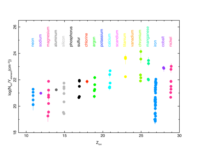
Figure 16: Element column densities obtained assuming linear curve of growth, cosmic element abundances, and unit ion fractions for all lines in Table 2. Each data point represents one line. The horizontal axis is the quantity $Z_{ion}$ where we distinguish between contributions of various ions by assigning $Z_{ion}=Z_{element}+1-0.1*(ionstage)$, where $(ionstage)$=1 for hydrogenic, 2 for He-like, etc. Element color coding is the same as in figure 15.

2.3 Curve of Growth

The validity of the procedure used to derive the columns in figure 16 depends on the assumption that the lines lie on the linear part of the curve of growth. If this is correct, then the line equivalent widths should be proportional to the transition oscillator strengths, and comparison of various lines from the same ion should show this proportionality. In figure 17 we test this procedure using the Lyman series lines from H-like ions of Ne, Mg, Al, Si, S, Ar, Ca, Cr, and Mn. We also include the $2s-np$ lines from Li-like Fe XXIV and Ni XXVI. Solid lines are linear regression fits to data with errors less than 0.1. Also shown on this figure are diagonal lines (dashed) corresponding to the proportionality expected for linear curve of growth. This shows that, although some ions appear to follow the linear trend, the strongest lines in particular grow more slowly than linearly. This is particularly apparent for the lines of Ne X, Fe XXIV and Ni XXVI. Each ion has at least 5 lines, and the trend is apparent across the line strengths. This shows that the simple analysis provided in figure 16 and Table 2 are likely not adequate for the purposes of inferring abundances and the lines may be saturated. On the other hand, weaker lines such as those of Si XIV do apparently follow the linear trend.

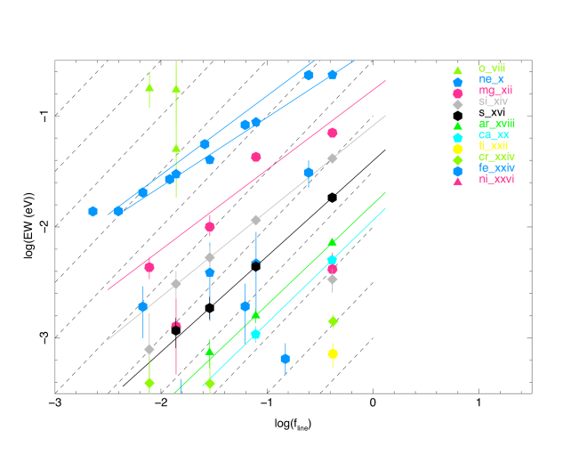
Figure 17: Curve of growth for H-like and Li-like ions. Element color coding is the same as in figure 15. Dashed diagonal lines show simple proportionality behavior expected for unsaturated lines. Solid lines are linear regression fits to data with errors less than 0.1.

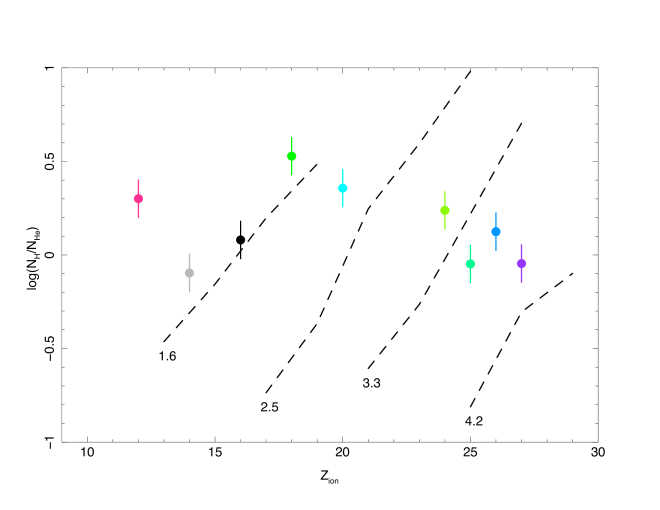
Figure 18: Ratio of column densities derived from linear curve of grow analysis for H-line to He-line ions, versus the nuclear charge. Element color coding is the same as in figure 15.

Another illustration of the effects of saturation is shown in figure 18. This shows the ratios of He-like to H-like ion abundances inferred from the line equivalent widths and identifications in Table 2. These ratios are independent of element abundance, owing to the fact that each ratio is taken between ions from the same element. This shows that the ratios are all in the range between 10^-1 and 10⁺¹ for $12\leq Z\leq 26$, but that there is no systematic trend with $Z$. We might expect the ratio to increase with $Z$, as higher $Z$ elements would be generally less highly ionized, for plausible ionization mechanisms. Also shown in figure 18 are the contours traced by an xstar photoionization model described in more detail in the Appendix. These are labeled by the value of log($\xi$), where $\xi=L/(nR^{2})$ is the ionization parameter as defined by Tarter et al. (1969); $L$ is the source energy luminosity integrated from 1 – 1000 Ry, $n$ is the gas number density, and $R$ is the distance from the continuum source to the absorber. These show that a given value of ionization parameter predicts that the He/H abundance ratio should increase between adjacent elements by a factor $\sim$5. The figure clearly shows that a single ionization parameter cannot account for the ratios displayed by all the elements. This could indicate the existence of a broad range of ionization parameters in the source, spanning values indicated by this figure. On the other hand, it could be associated with radiative transfer effects, such as saturation, which make ion fractions inferred from a linear curve of growth unreliable.

Possible explanations for the departures from the linear curve of growth include the influence of saturation which causes the curve to flatten when the lines become optically thick in the Doppler core. Other possibilities include filling-in of the lines by an additional continuum emission component which is not seen in transmission through the warm absorber, and also radiation transfer effects in the absorber itself. The latter includes forward scattering, which may also depend on the relative size of the continuum source and the absorber. Also, thermal emission can fill in the lines. In the following subsection we discuss these in turn.

2.4 Radiation Transfer and Curve of Growth

The standard curve of growth for a resonance line can be written:

$$EW=\int{d\varepsilon\left(1-e^{-\tau(\varepsilon)}\right)}$$ (2)

$$\tau(\varepsilon)=\frac{\pi e^{2}}{m_{e}c}fx_{ij}Y_{j}N\frac{\lambda}{v_{turb}}\phi(\frac{\varepsilon}{\Delta\varepsilon_{turb}})$$ (3)

where $\varepsilon$ is the photon energy, $f$ is the oscillator strength, $x_{ij}$ is the ion fraction, $Y_{j}$ is the element abundance, $N$ is the total column density, $\lambda$ is the line wavelength, $v_{Turb}$ is the turbulent velocity (including the thermal ion speed), and $\phi$ is the profile function, which includes both a Doppler core and damping wings. This is shown in figure 19, for various choices of the velocity characterizing the Doppler broadening $v_{turb}$, and for a natural width corresponding to that for the Si XIV L$\alpha$ line. This shows that, for a given equivalent width, the effects of saturation are more likely to be important when the Doppler broadening is smallest. That is, the equivalent width where the curve flattens is approximately proportional to the Doppler width. As we will show, the widths of many lines from GRO J1655-40 are not constrained from below by the HETG spectrum. Thus, a possible explanation for the slower than linear curve of growth is that the line Doppler widths are small enough such that the strongest lines in figure 17 are affected by saturation.

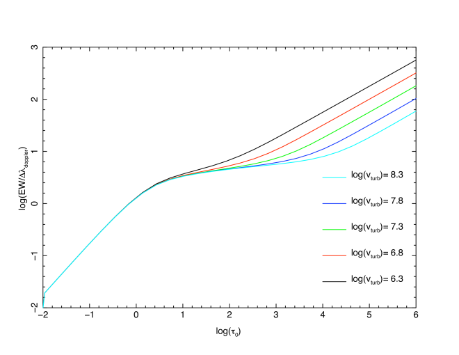
Figure 19: Curve of growth for various choices of the velocity characterizing the Doppler broadening $v_{turb}$, and for a damping parameter corresponding to that for the Si XIV L$\alpha$ line, at a Doppler broadening velocity of 20 km s^-1.

Filling in by continuum from a separate source which is not absorbed by the warm absorber would preferentially affect lines with larger optical depths. This could qualitatively explain the flattening of the curve of growth which is observed. However, the filling in would also have the wavelength dependence of the additional continuum component. Although this is unknown, the simplest assumption would be that it is the same as the primary continuum. We have tested this possibility quantitatively using direct fitting, and will discuss this further in the following section.

The standard curve of growth in equation (2) assumes the simplest possible geometry and microphysics affecting the line: (i)The continuum source has negligible size; (ii) The absorber exists only in a narrow region along the line of sight to the continuum source; (iii) The excitation and deexcitation of the transition responsible for the line is affected only by the radiative excitation and spontaneous decay connecting the two atomic levels. In addition, the gas is assumed to have a velocity field which can be characterized by a Maxwellian distribution with a well-defined thermal or turbulent velocity.

If the continuum source has finite size, or if the warm absorber exists outside the line of sight to the source, then the line profiles will be affected by photons which scatter into our line of sight. Although there is no simple general expression for the intensity observed from an extended scattering atmosphere in this case, it is straightforward to show that in the limit of small optical depth, the scattered emission contribution scales proportional to $(D/R)^{2}$, where $D$ is the characteristic size of the continuum source and $R$ the characteristic distance from the continuum source to the absorber. This contribution is independent of optical depth in this limit, and so will not affect the shape of the curve of growth at small $\tau$.

Departures from assumption (iii), concerning the population kinetics, can be expected if the radiative decay of the upper level is suppressed or if the upper level can be populated by another process such as recombination or collisional excitation. Some of these possibilities were discussed by Masai & Ishida (2004). If the upper level can decay via alternate channels, such as branching to other levels radiatively, collisional deexcitation, or autoionization, the basic absorption profile properties will be unchanged (although these processes can affect the damping parameter). Suppression of the upper level decay by collisional deexcitation could occur if the product of line optical depth and electron density, $n_{e}$, is large, but this requires optical depth $\sim 10^{18}/n_{e}$ for iron. This would affect our limits on possible filling-in of the line by collisional or recombination radiation which we present in the next section. Populating the upper level by collisions or recombination requires suitable temperature and ionization conditions. Efficient population by collisional excitation requires temperatures greater than can be accounted for by photoionization heating and radiative cooling, and this in turn will affect the ionization balance. It also implies the existence of an additional heating mechanism. We have tested these possibilities quantitatively using direct fitting, and discuss the results below.

3 Direct Fitting

Many of the issues discussed in the previous section can be tested using direct fitting. These include: detector resolution, counting statistics, and scattered and thermal (either collisional or recombination) emission. In order to do so, we use the warmabs analytic model which interfaces with the xspec spectral fitting package. warmabs makes use of a stored, precomputed table of level populations for a family of photoionization models. It uses these to calculate a synthetic spectrum ‘on the fly’ within xspec. The advantage of this is that it calculates the synthetic spectrum automatically for the energy grid of the data such that it matches the energy resolution of the instrument. Interpolation can introduce significant numerical errors when applied to absorption spectra, since the absorption coefficient can change rapidly over a narrow range in energy. Warmabs calculates all absorption lines using a Voigt function including damping due to both radiative and Auger decays where applicable. Line profiles are calculated using sub-gridding, on an energy scale which is a fraction of a Doppler width, and the opacity and transmittivity then mapped onto the detector grid. Bound-free absorption is also included. Warmabs uses the full database and computational routines from the xstar package (Kallman and Bautista, 2001; Bautista and Kallman, 2001), and differs from xstar in that the level populations are pre-calculated rather than calculated simultaneously with the spectrum. The level populations are calculated using a full ‘collisional-radiative’ calculation, albeit with relatively simple model ions in most cases. Thus they include the effects of upper level depletion due to thermalization and photoionization automatically. We have extended the xstar database to include all the trace elements seen in the GRO J1655-40 spectrum. A description is provided in the Appendix.

Warmabs does not calculate the flux transmitted by a fully self-consistent slab of gas, as xstar does. Rather, it calculates the opacity from the illuminated face of such a slab, and then calculates optical depth and transmitted flux analytically by assuming the opacity is uniform throughout the slab. A real slab will shield its interior, which will then have lower ionization and greater opacity than a slab whose opacity is assumed to be uniform. Thus, the results of warmabs fitting will be absorbing columns which may be greater than would be produced by a real slab. The importance of this effect depends sensitively on the assumed slab structure, i.e. its geometrical thickness, and so its importance cannot be estimated in general. Also, this effect is negligible at high ionization parameters. As we will show, our fits require large ionization parameters. In this case, the advantages of the energy resolution provided by warmabs outweigh its limitations.

3.1 Model 4: Narrow Lines

Our basic fit assumes that the absorption is provided by a single component of photoionized gas. We adopt the ionizing continuum used by Miller et al. (2008) which consists of a power law plus disk blackbody, as described in the previous section. The power law photon index is 3.54 and the disk inner temperature is kT=1.35 keV. In our fit we account for the curve of growth by adopting a small turbulent velocity, 50 km s^-1, so that the ratios of these lines are on the saturated part of the curve of growth. We then search for the single ionization parameter which most nearly accounts for all the lines in the spectrum. We do this using warmabs and the xspec package and stepping through ionization parameter in intervals $\Delta$log($\xi$)=0.1. Warmabs accept the turbulent velocity as an input, but the actual line width is calculated including both this turbulent velocity and the thermal ion velocity corresponding to the equilibrium temperature. As shown in the Appendix figures 23 – 26, in order to simultaneously produce the ions of iron ranging from B-like (Fe XXII) to H-like, an ionization parameter in the range 3$\leq$log($\xi$)$\leq$4 is needed. We find the best fit at log($\xi$)=4.0${}^{+}_{-}$0.1, log(N)=23.8 and a blueshift for the absorber of 375 km s^-1. This can be compared with the radial velocity of the system of 141${}^{+}_{-}$1 km s^-1 and the orbital semi-amplitude of the secondary star of 215.5 ${}^{+}_{-}$2.4 km s^-1 (Shabhaz et al., 2002). This suggests that the outflow is not moving fast when compared with the maximum velocities characterizing the orbital motion in the system. We have also performed equivalent fits for this set of assumptions using the isis fitting package (Houck & Denicola, 2000), and have verified that the results are independent of which fitting package is used.

We refer to this single component warmabs with $v_{turb}=50$ km s^-1 as model 4. We assume a gas density of 10¹⁵ cm^-3 in calculating the level populations used by warmabs. We have not extensively tested our results at lower densities, and we point out that it is likely that densities as low as $10^{13.8}$ cm^-3 can produce the Fe XXII lines. We employ the same ionizing continuum as derived in the model 1 fit when calculating the populations and gas temperature using xstar. In our fitting for model 4 and subsequent models we allow the normalizations of the two continuum components to vary. The best fit flux is 1.8 $\times 10^{-8}$ erg cm^-2 s^-1 in the 2 – 10 keV band. In Figures 1-14 we show the observed count rate spectrum (black) together with all the models discussed in this section as red curves, labeled according to the model number. Strong lines are marked in blue along with parent ion.

As discussed above, and shown in figure 15, the majority of lines have centroid wavelengths which are consistent with a single Doppler blueshift, approximately 400 km s^-1 with respect to their laboratory values. The notable exception is the Fe XXVI L$\alpha$ line near 1.77 Å  which has a centroid wavelength corresponding to a Doppler blueshift of $\simeq$1300 km s^-1. In model 4, we adopt the hypothesis that this line arises in a separate velocity component of the flow, which must have a much greater ionization parameter so that it does not show up in the other lines. Since the xstar grid of model level populations does not extend to values where Fe XXVI is the only ion of significant abundance, we do this by adding a single Gaussian component for the high velocity part of this line. A consequence of this is that the 375 km s^-1 component of the flow, which we model with warmabs and an ionization parameter log($\xi$)=4, accurately fits to the red part of the Fe XXVI L$\alpha$ profile, while the Gaussian accounts for the rest. This is shown in figure 20, which shows the region surrounding the line. The data is shown as the black bars, and model 4 is shown as the dark blue points. The green points show the continuum + Fe XXVI L$\alpha$ Gaussian model alone. The equivalent width of the Fe XXVI Gaussian is 29.6 eV. The $\chi^{2}$ for this model is 34211 for 8187 degrees of freedom. These parameters are summarized in Table 1.

An alternative possibility is that the Doppler blueshift of the Fe XXVI line is affected by instrumental effects and shortcomings in the available HETG response function. This could be due to the fact that the continuum count spectrum is steeply decreasing in the line region, as shown in figure 20. Internal scattering could cause photons from the continuum adjacent to the longer wavelength wing of the line to scatter into the line core, and this effect would be stronger on the long wavelength side than on the short wavelength side. The width of the line spread function is comparable to the line blueshift. In addition, the wavelength calibration may be affected by the use of continuous clocking mode. On the other hand, other lines in the 1.5 – 2 Å region, although at slightly longer wavelength, do not show this effect, as exemplified by the Fe XXV $1s^{2}-1s2p$ line. Furthermore, we have confirmed that the response matrix we use reproduces the line spread function obtained from the $Chandra$ calibration database . So, although there is no obvious shortcoming in the response matrix which would explain the discrepancy between the Fe XXVI L$\alpha$ wavelength shift and those of other lines, we will examine both hypotheses: that the high velocity part of the Fe XXVI line is associated with a separate kinematic component (as in model 4), and that it is not. The latter case also corresponds to the assumptions of Miller et al. (2008). The primary conclusions of this paper, with respect to dynamics, abundances, turbulence, and geometry, are not dependent on this assumption.

The model 4 fit accurately reproduces the strength and shape of the Fe XXVI and Fe XXV lines, although we predict a slightly stronger red wing on the Fe XXV than is observed. This is the contribution of Fe K$\alpha$ from lower ion stages of iron, Fe XXIV and XXIII. The strengths of these lines provides a lower bound on the ionization of iron. We also slightly overestimate the strength of the Mn XXV L$\alpha$ line, relative to the Mn He-like K$\alpha$ line. This may be due to an error in the ionization balance for this element; as shown in figure 18, there are apparent departures from a simple monotonic trend in the H/He ratio with nuclear charge. The region longward of 3Å includes the lines from Ca (3.02, 3.18 Å) and Ar (3.73, 3.94 Å). Our single component ionization balance is too low for both these elements, adequately accounting for the He-like lines but under-predicting the H-like lines. We also point out that our assumed line width of 50 km s^-1 adequately fits the profiles of essentially all the lines shortward of 6 Å.

Model 4 is based on a physical model for the absorber in GRO J1655-40, and it represents the best fit that we can obtain to the spectrum using a single warmabs component. As shown in figure 1-14, this accounts for the depths and positions of essentially all the lines in the spectrum. Discrepancies between the model and the data fall in three categories: errors in the continuum, errors in line widths, and errors in line strengths (including lines which are missing). In what follows we will explore these in turn. As we will show, the best fits we obtain to a physical model have $\chi^{2}/\nu$ $\sim$ 2.9. This can be compared with the phenomenological notch fit, model 3, which has reduced $\chi^{2}/\nu$ $\sim$ 2.2. The difference likely represents the ability of the phenomenological notch fit to account for features which may not be physical lines but rather part of the continuum or consequences of calibration uncertainties. This, we think, represents the ultimate limit in our ability to fit the spectrum. In what follows, we proceed and attempt to interpret the $\chi^{2}$ values from physical models when compared with each other, but without relying on standard interpretations of these values and their relation to probability of random occurrence, etc. That is, we acknowledge that our fits are not acceptable based on these standard arguments about $\chi^{2}$, but nevertheless interpret confidence intervals on the fitting parameters by evaluating $\Delta\chi^{2}$ as if they were.

Model 4 is designed to fit to the curves of growth of lines from Fe XXIV and Ni XXVI by having a relatively small turbulent velocity, so that the lines from these ions are at least partially saturated. This works for these ions, as is apparent from figure 6, and it also is consistent with the observed widths of the lines which are not resolved. However, it does not account for the observed widths of the broader lines, such as Si XIII and Si XIV, and also for the 2s – 3p lines of Fe XXIV near 10.6 Å. Miller et al. (2008) adopt a line width of 300 km s^-1, which is a better fit to the observed widths for many lines. We conclude that saturation with a single profile component, although it accounts for the curves of growth of the lines of Fe XXIV, is not consistent with the curves of growth of lines from Si XIV, nor is it consistent with observed widths of some of the strong lines. A possible explanation is that the lines consist of multiple narrow components closely spaced in velocity so they appear blended together in the HETG, and where the components furthest from line center are unsaturated and so appear only in the low members of the Li-like 2s – np series. UV warm absorber lines in AGN appear to follow this behavior (Gabel et al., 2005).

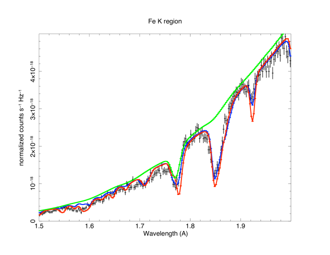
Figure 20: detail of spectrum in the 1.5 – 2 Å region. Crosses are data, blue is model 4, red is model 5, green is the Fe XXVI L$\alpha$ Gaussian contribution to model 4.

3.2 Model 5: Two components plus broad lines

Another way to fit the Fe XXVI L$\alpha$ line is to add a higher ionization parameter warmabs component to the fit. We do this in model 5, which has a warmabs component with the same ionization parameter as model 4, but with the addition of a second component at an ionization parameter which can make the Fe XXVI line sufficiently strong without over-producing the lower ionization lines. This model also has a turbulent velocity of 200 km s^-1. We vary the column densities and element abundances of both components in order to find the best fit. In doing so, we force both components to have the same bulk outflow velocity, the same turbulent velocity, and the same elemental abundances. Thus, the two components are allowed to differ only in their ionization parameters and column densities. This produces a fit with $\chi^{2}/\nu=36281/8189$. This fit is also shown in figures 1 – 14. In figure 20 we show a blowup of the iron K region, comparing this model with model 4. Model 4 is decomposed into the part accounted for by the Gaussian (green) and the total (blue). Model 5 is shown as the red points. This shows that in spite of the nearly equivalent $\chi^{2}$, model 5 does less well than model 4 in fitting the iron lines; it generally over-predicts their strengths. This is particularly true in the case of the Fe XXVI L$\alpha$ line. Since this model has the same 375 km s^-1 outflow velocity as model 4, the best fit accounts for the blue edge of the Fe XXVI L$\alpha$ by over-predicting the line near line center and the red edge. Thus, the conclusions from this model differ from model 4 (and subsequent models) in that they do not depend on the existence of two kinematic components.

In other ways, the comparison between models 5 and 4 reflects the fact that model 5 has on average a higher ionization parameter. As a result, model 5 tends to over-predict the ratio of H-like to He-like lines, compared with both model 4 and with the observation. Also, model 5 has a larger turbulent velocity, and therefore predicts a steeper curve of growth for most lines. This fact is apparent from the Fe XXIV lines in the 6 – 7 Å region. On the other hand, model 5 fits better than model 4 to lines which appear to follow the linear curve of growth, such as the L$\beta$/L$\alpha$ lines of Si XXIV, and also to lines which are detectably broadened, such as the 10.6 Å doublet of Fe XXIV.

3.3 Model 6: Partial Covering

An additional possible reason for the apparent saturation of the curves of growth could be due to systematic effects or calibration uncertainties associated with the $Chandra$ telescope, grating and detector. This could lead to apparent scattering of photons in the continuum into the cores of absorption lines which is not accounted for by the detector response matrix, thus preventing the residual flux in the lines from going to zero. This effect cannot be evaluated accurately without calibration data which includes narrow absorption line features, but we can get an indication of its plausibility by fitting to a model which includes some ‘leakage’ of photons into lines from adjacent continuum regions. We do this by fitting to a partial covering model in which the warmabs component is partially diluted, i.e. $model=((1-C)+C\times{\sc warmabs})\times continuum$ where $1-C$ is the fraction of scattered continuum at each energy. We also adopt a turbulent velocity of 200 km s^-1 for this model, since we do not need to account for saturated curves of growth; the dilution of the warmabs lines tends to flatten the curves of growth. We show this as model 6 in Table 1 and in figures 1 – 14. This model has $\chi^{2}/\nu=24561/8184$, and so is the best of the fits using the warmabs model. It also employs a turbulent velocity which is sufficient to account for the widths of resolved lines while at the same time fitting to the curves of growth for Fe XXIV and Ni XXVI.

The best-fit value of $C$ is 0.37. We can interpret this as being due to true partial covering in the object, i.e. if the continuum source is more extended than the absorber, or as being due to instrumental scattering which is not accounted for by the response matrix we used. The latter can be further subdivided into shortcomings in the response in accounting for the line spread function (LSF) for the HETG which occur in the core region of the LSF, and shortcomings which occur in the wings. The core region of the LSF . can be approxmiately represented by a Gaussian with full-width-half-maximum (FWHM) of $\simeq$1300 km s^-1 at the wavelength of the iron line, 1.77 Å. So two intrinsically narrow lines of equal intensity will fill the region between them to 30$\%$ of their peak intensities if they are separated by $\simeq$ 900 km s^-1. This is comparable to the typical line widths we find in our fits. However, as discussed previously, the response matrix we use does accurately reproduce the LSF in the core region, so it would require a large error in the calibration files, the LSF and the resulting response matrix, in order to account for the filling in of the lines in this way.

Another possibility is that there exists significant scattering in the line wings which is not accounted for by the calibration. This is difficult to evaluate quantitatively, except to point out that the uncertainty in the LSF at the extremes of the wings appears to be at most $\sim$2 – 4 $\%$ of the maximum value. In order to make up the covering fractions we require, the integrated area under the wings would have to be $\sim$30 – 40 $\%$ of the area in the core of the line. The wings would have to extend to $\simeq$10 times the $\sigma$ of the core, or $\simeq$7600 km s^-1. We cannot evaluate the likelihood of this possibility reliably, and cannot conclusively rule it out, although such a large departure from the calibration would be surprising. This observation differs from typical observations in its use of continuous clocking mode. This prevents the use of detector regions adjacent to the readout strip for background subtraction, but the counting rate in this case is high so that background should not be important at the levels considered here. The fact that the response matrix agrees with the LSF in the core of the line is further evidence that the use of continuous clocking is not the source of the apparent partial covering.

We conclude that true partial covering in the source is more likely than instrumental effects, and thus plays a role in determining the line curves of growth and the overall quality of the fit. Owing to its superior $\chi^{2}$ we adopt this model as the one which most nearly accounts for the observed spectrum and consider the physical assumptions to be most nearly correct for the GRO J1655-40 outflow. We emphasize that the partial covering does not account for the high velocity component in Fe XXVI L$\alpha$, and model 6 includes the same high velocity Gaussian contribution to this line as model 4.

3.4 Other Models

We also have examined the possible influence of thermal emission filling in lines on the one-component warmabs fit, i.e. model 4. That is, we have included an additional emission component, which emits due to ‘thermal’ (i.e. collisional and recombination) processes rather than resonance scattering. This component is calculated using the photemis model, and is the emission analog of warmabs. It is assumed to have the same ionization parameter, abundances, redshift, and turbulent velocity as the warm absorber component. We allow the normalization of the emission component, which is proportional to its emission measure, to vary, along with the optical depth of the warm absorber. In doing so, we find the best fit to be that with zero thermal emission, and the statistical upper limit on the thermal emission component corresponds to an emission measure $EM\leq 1.2\times 10^{56}$ cm^-3. We will discuss the implications of this in the next section.

We have also examined the possibility that the absorption is produced in a plasma which is in coronal equilibrium instead of photoionized. This is what might be expected if the gas is heated mechanically, and if the outflow is due to thermal expansion of such a mechanically heated wind. This is done using the xspec analytic model hotabs, which calculates the absorption spectrum of partially ionized gas if the ionization is due to electron impact. The free parameter describing the ionization balance in this gas is the electron temperature. A key difference between a photoionized gas and a gas in coronal ionization equilibrium is that the ionization abundance distributions from photoionized gas have more overlap in parameter space than does a coronal gas. That is, at a given temperature each element in a coronal gas is most likely to exist in a pure ionization state, while at a given ionization parameter in a photoionized gas, each element is likely to have a mixture of two or more ionization states. In addition, the ions which can coexist in a coronal plasma all tend to have similar ionization potential. A consequence is that it is impossible for coronal equilibrium to allow the coexistence of H-like or He-like ions of elements with very different nuclear charge, eg. Fe XXV and S XVI. In contrast, a photoionized plasma at log($\xi$)=4 does allow this. For this reason, coronal equilibrium models do not fit the GRO J1655-40 spectra as well as photoionized models.

3.5 Abundances

We have also varied the elemental abundances and explored the limits for these allowed by the $\chi^{2}$ statistical criterion. In doing this, we rely on the criterion of Cash (1979), where a 99$\%$ confidence interval is defined by the values of the parameter which fall within $\Delta\chi^{2}\leq 10$ of the best fit value. We display these results graphically in figure 21 for the elements O – Ni. The abundances here are taken relative to the solar values of Grevesse et al. (1996) for abundant elements, and Allen (1973) for the new elements added for this calculation. In all of our models we fix the abundance of Fe at 1 relative to solar. In Figure 21 the results of model 4 are shown in black, and the results of model 6 are shown in red. This shows that the models agree on the abundances of elements Sc through Co, such that the abundances of Cr, Mn and Co are all enhanced relative to Fe by at least 50 $\%$. For Ca model 4 predicts values greater than solar by 0.5-1 dex while model 6 is consistent with solar. As discussed above, we conclude that model 6 most nearly fits the overall properties of the spectrum, and in what follows we discuss the implications of the abundance pattern from this model. Limits on the abundance of O come from the O VIII 1s – 5p line at 14.8 Å and 1s – 6p at 14.64 Å. This results in $Y_{O}$ values in the range 0.2 – 1.5.

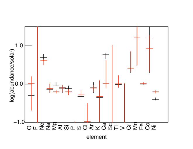
Figure 21: Element abundances: model 4(black) and model 6 (red). log(abundance)=0 corresponds to solar Grevesse et al. (1996) values.

The abundance patterns shown in figure 21 are crudely consistent between models 4 and 6, and show enhanced abundances of Cr and Mn relative to Fe. Results for Ca-V are ambiguous, and suggest no strong enhancement, while the abundances of Na-Cl are smaller than the solar ratio, relative to Fe.

The overabundances of Fe-group elements strongly suggest that the observed matter has been subject to high-temperature burning conditions. For this reason, we have compared the observed abundances against nucleosynthesis models in massive stars, and more particularly resulting from the hydrostatic C-, O- and Si-burning phases. We use the presupernova nucleosynthesis yields calculated in model stars of 15, 20, and 25 solar masses with solar metallicity (Limongi et al, 2000). Each of the C-, O- or Si-burning zone has been weighted by the relative masses needed to best reproduce the observations. The relative mass ratio (C:O:Si) obtained is (6:1:1) for the three model stars. As shown in Fig.  22, the predicted abundances (relative to solar) are in rather close agreement with the observed pattern for models 4 and 6.

As far as the light elements are concerned, the agreement between theory and observation is rather good. The O overabundance predicted reaches 1.3 (1.8 for the 20 M_⊙ star) in agreement with the 1.5 upper limit determined in the 2-component model. Note, however, that the O abundance is not well constrained by the observed spectrum owing to strong interstellar absorption. Furthermore, we consider it possible that the low $Z$ elements are affected by a separate ionizing continuum component. This could suppress absorption from O even if the abundance were greater than solar, although this is contrived given the absence of observations of such radiation. We also point out the possibility that the Ne and O lines are at least partly of interstellar origin (e.g. Juett et al. (2004)). This would require a coincidence in velocity between the GRO J1655 outflow and the intervening gas. It would also place more severe constraints on the nucleosynthetic models, since it would decrease the inferred abundances of these elements intrinsic to the source.

Concerning the underproduction of Na, the disagreement may be due to uncertainties affecting the nuclear reaction rates or the thermodynamical conditions in the combustion zones. For the heavier elements above Ca, the agreement is still good though discrepancies can be seen in particular for Ti, V, and Co. It should be mentioned here that, in the nucleosynthesis simulations, all unstable nuclei produced have been assumed to $\beta$-decay (except the long-lived ⁵³Mn).

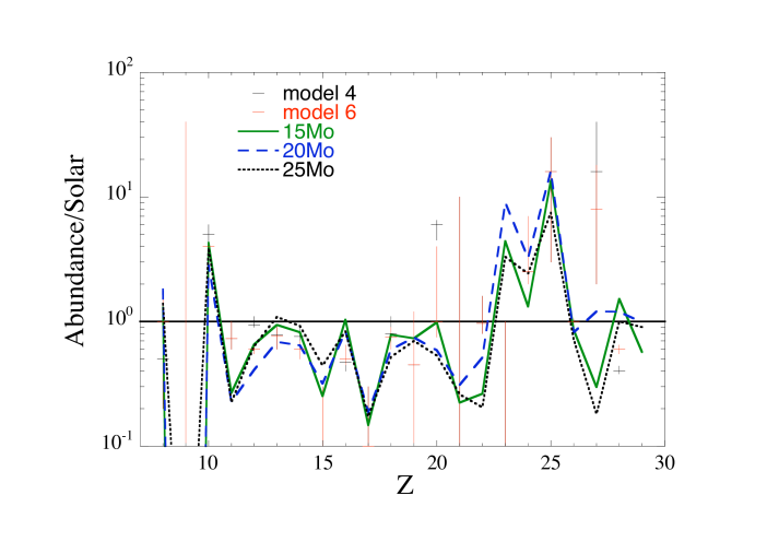
Figure 22: Comparison of observed and predicted overabundances. The symbols with errors bars correspond to the 1-component (black) and 2-component (red) models. The lines correspond to model calculations in a 15 M_⊙ (solid), 20 M_⊙ (dashed) and 25 M_⊙ (dotted) star, as described in the text.

It is interesting to compare with the results of the optical abundance determination by Israelian et al. (1999). These authors find evidence for enhanced O/H, Mg/H, Si/H, S/H relative to solar, but Fe/H and Cr/H are approximately solar. This differs from our results for models 4 and 6, insofar as they can be compared, since Israelian et al. (1999) do not measure abundances for Mn, Co, and Ni. The conclusions of Israelian et al. (1999) have not been confirmed in an investigation by Foellmi et al. (2007). This also underscores the fact that the abundances we measure are relative to each other, and all are for elements heavier than O. We have assumed that iron is solar and quote other abundances relative to that, but we have no constraints on abundances for light elements, or for any abundances relative to hydrogen.

4 Discussion

Other implications of our models include the fact that the curves of growth, in the absence of partial covering, indicate a velocity structure which has a small turbulent velocity, $\simeq$50 km s^-1 at the same time as a larger bulk velocity, $\simeq$400 km s^-1 . Since the radial velocity of the GROJ1655-40 system is 141${}^{+}_{-}$1 km s^-1, this implies an outflow consisting of material which is cold or still compared with the bulk flow. This is unusual when compared with flows which are well studied in stars and non-thermal outflows from compact objects.

All of our models fit to the iron K region by assuming the existence of a separate, higher ionization component which is primarily responsible for producing the Fe XXVI L$\alpha$ line. This is because essentially all the other lines in the spectrum are consistent with a single ionization parameter and outflow velocity. Models 4 and 6 fit the Fe XXVI L$\alpha$ line using an ad hoc Gaussian, while model 5 fits it using a separate warmabs component. Although the latter approach is more physically consistent, it does not fit the feature as well because for this model we force the two components to have the same outflow velocity.

In either case, we find that the majority of lines fit to a single ionization component, log($\xi$)$\simeq$4. In addition to this, we have the observed luminosity $L\simeq 5\times 10^{37}$ erg s^-1 (Miller et al., 2008) and density constraints from the Fe XXII metastable line implying $n\geq 10^{14}{\rm cm}^{-3}$. Taken together, these determine the location of the absorber: $R=\sqrt{L/n/\xi}\simeq 10^{9}L_{37}^{0.5}n_{15}^{-0.5}\xi_{4}^{-0.5}$ cm, and its size: $\Delta R=N/n\simeq 10^{9}N_{24}n_{15}^{-1}$ cm. In these equations $L_{37}$ is the luminosity in units of $10^{37}$ erg s^-1, $n_{15}$ is the density in units of 10¹⁵ cm^-3 and $\xi_{4}=\xi/10^{4}$. That is, for plausible values, $R\leq 7\times 10^{9}$ cm, $\Delta R\leq 10^{10}$ cm. This location can be compared with the ‘Compton radius’ within which photoionized gas cannot escape the gravity of the black hole (Begelman et al., 1983), which is $R_{IC}=10^{10}(M/M_{\odot})T_{IC8}^{-1}$, where $T_{IC8}$ is the temperature of the photoionized gas in units of 10⁸K, and for the GRO J1655-40 spectrum this value is $\leq$0.03 and the mass of the black hole is 5 – 8 $M_{\odot}$. If so, $R_{IC}\simeq 2\times 10^{12}$ cm. Thus the inferred wind location is well within the Compton radius and is inconsistent with an outflow driven by thermal expansion, even though weak flows are possible at $\sim 0.1R_{IC}$ as stated by Woods et al. (1996). This conclusion is consistent with that of Miller et al. (2008).

On the other hand, we note that the virial radius corresponding to the outflow speed we measure is 1.3 $\times 10^{12}$ cm, considerably greater than the position we infer from the X-ray ionization balance. This, together with the fact that the outflow speed is comparable to the orbital speed in the system raise the possibility that the outflow could be associated with the secondary star or a region of the binary which is at comparable distance from the black hole. If so, then the radius we infer from the ionization balance arguments is an underestimate. This is difficult to understand in view of the density constraints from the Fe XXII lines; it would require that the metastable level of Fe XXII were populated by radiative pumping rather than by collisions. This, in turn, would require that the intensity of the radiation in the $\sim 100\AA$ region to be close to LTE, and there is no known source for such radiation far from the black hole. In addition, the observed outflow speed does not appear to vary during the observation (Miller et al., 2008), which spanned $\simeq$20$\%$ of an orbital period, which argues against an origin associated with the companion star or accretion stream. Thus, we consider this possibility to be unlikely.

Another astrophysical system which appears to show a comparable contrast between line turbulent width and outflow velocity are FU Orionis stars. In these systems the terminal velocity of the wind is 300-400 km/s, and the rotational broadening (seen in absorption) of the wind is about 50 km/s (Calvet et al., 1993; Hartmann & Calvet, 1995). The intrinsic turbulent velocity needed to produce the lines is likely much smaller. If so, the contrast between outflow and turbulent velocities is comparable to the contrast between the observed width and the virial speed at the inferred position for the GRO J1655-40 outflow.

We note also that the flow timescale is $t_{dyn}=R/v_{out}\simeq 27$s. This can be compared with the recombination timescale $t_{rec}=(n\alpha)^{-1}\simeq 10^{-4}$s, showing that the assumption of ionization equilibrium is valid for these simple assumptions about the density and location of the outflow. This does not change qualitatively if the absorber is located at the virial radius.

We can also explore the implications of the emission measure upper limit derived in the previous section, $EM\leq 1.2\times 10^{56}$ cm^-3. The emission measure expected from a constant density shell with size derived from the ionization parameter, density and thickness is $EM=10^{57}\Omega L_{37}N_{24}\xi_{4}^{-1}{\rm cm}^{-3}$, where $\Omega$ is the solid angle of the warm absorber/emitter. So we infer $\Omega\leq 0.12L_{37}^{-1}N_{24}^{-1}\xi_{4}$ or $\Omega\leq 0.024$ for the most likely value of $L_{37}$. This can be compared with the constraint derived by Miller et al. (2006) which is $\Omega\leq 1.4$ based on the observed limit on the Fe XXIV 2p – 3s emission line at 11.43 Å. We can also then estimate the mass loss rate in the outflow: Ṁ$=\Omega R^{2}nm_{H}v_{out}=2\times 10^{15}N_{24}^{-1}v_{7}$ gm s^-1 where $v_{7}$ is the outflow speed in units of 100 km s^-1; so Ṁ$\simeq 8\times 10^{15}$ gm s^-1 for our fits. This is small compared with the mass accretion rate required to fuel the X-ray source, Ṁ${}_{acc}\simeq L/(\eta c^{2})\simeq 6\times 10^{17}$ gm ^-1. The Miller et al. (2006) limit on the solid angle allows a considerably larger mass loss rate, $\leq$10$\%$ of the accretion rate.

Another conclusion of our work is the existence of two velocity components, one with ionization parameter log($\xi$)=4 and speed $v$=375 km s^-1 relative to the Earth, and the other with higher speed and much greater ionization parameter. We find for this second component a speed $\simeq$1400 km s^-1, and infer that the ionization parameter be high enough that Fe XXVI and Ni XXVIII are the only ions with appreciable abundance, say log($\xi)\geq 6$. Then the mass flux is Ṁ= $10^{17}\xi_{6}^{-1}v_{8}\frac{\Omega}{4\pi}$ gm s^-1, where we have assumed a source luminosity 5 $\times 10^{37}$ erg s^-1 and $v_{8}$ is the speed in units of 1000 km s^-1. It is more difficult to constrain the fractional solid angle of this component than it is for the lower ionization component because any emission may be masked by the lower velocity component, and we have not attempted to test this. It is clear that this component can carry more mass than the low ionization component if its solid angle exceeds 0.02. However, the radial location of this component cannot be reliably established, since the features in the spectrum which provide density constraints do not share the outflow velocity of this component.

The results found here agree qualitatively with those of Miller et al. (2008) in the sense that the ionization parameter and density of the flow containing most of the lines imply a wind location which is too close to the black hole to be easily explained by a driving thermal mechanism. We favor a scenario in which there are two components to the flow, and the lower ionization component is somewhat less ionized and the higher ionization component is more ionized than the single component found by Miller et al. (2008). Our spectral fitting allows us to constrain elemental abundances, and we find enhanced abundances for several elements in the iron peak. We do not find a pattern of systematic enhancements for $\alpha$-capture elements.

Appendix A Appendix: Photoionization Models

In order to model the spectrum of GRO J1655-40 we have made modifications and enhancements of the xstar photoionization code (Kallman and Bautista, 2001). This code calculates the transfer of X-rays and other ionizing radiation, and the ionization balance, opacity and reprocessed emission from gas under a variety of physical conditions. It contains a relatively complete and up-to-date collection of atomic cross sections, rate coefficients and atomic energy levels. The code and atomic database, along with the ‘warmabs/photemis’ analytic models for xspec, are freely available, distributed as part of the ftools package, and have been widely used in interpreting X-ray spectra.

The standard xstar distribution includes all abundant even-$Z$ elements (plus N), i.e.: H, He, C, N, O, Ne, Mg, Si, S, Ar, Ca, Fe and Ni. In order to model GRO J1655-40 we have added all the other elements with $Z\leq 30$, with the exception of Li, Be, and B. The atomic data needed to do this, in addition to the resulting ionization balance for an optically thin gas, are discussed in this appendix. These data include: energy levels, line wavelengths, oscillator strengths, photoionization cross sections, recombination rate coefficients, and electron impact excitation and ionization rates. Distorted wave dielectronic and radiative recombination rate coefficients, photoionization cross sections, and photoexcitation-autoionization rates have been calculated (Badnell et al., 2003) for ions of these elements belonging to the H-like through Na-like isoelectronic sequences and are also available in the ORNL ADAS database (Schultz, et al., 2000). Concerning the other atomic parameters, a survey of atomic databases (Kallman and Palmeri, 2007) reveals that they are far from complete for any of these elements. Therefore we rely heavily on hydrogenic scaling for many of these quantities.

In order to model the spectrum we have modified the xspec analytic model warmabs in order to account for the new elements. warmabs uses the optically thin ionization balance calculated by xstar, along with the same atomic database as xstar, to calculate the synthetic spectrum expected for a gas seen in transmission with a given ionization parameter, column density, turbulent velocity and abundance set. This takes into account all of the absorption processes, i.e. lines and photoionization cross sections, included in xstar. A complementary model, photemis, calculates the emission spectrum expected from such a gas, but that is not used in the calculations presented here.

Rates and atomic structure for elements H, He, C, N, O, Ne, Mg, Si, S, Ar, Ca, Fe and Ni are the same as those described in (Kallman and Bautista, 2001; Bautista and Kallman, 2001), and available in version 2.1l of the xstar code (http://heasarc.gsfc.nasa.gov/docs/software/xstar/xstar.html). For the odd-$Z$ elements, and the iron peak elements not included in the release version of xstar, we use atomic structure scaled according to the following prescription: for the H- and He-like isoelectronic sequences we scale all energies and rates according to that expected for hydrogenic quantities: energies scale according to $Z^{2}$, photoionization cross sections scale according to $Z^{-2}$, transition probabilities scale according to $Z^{4}$. For these isosequences we scale the full atomic structure and rate set from xstar, including all levels through $n=6$ for hydrogenic and through $n=5$ for helium-like ions. For other isoelectronic sequences we adopt hydrogenic scaling of a highly simplified hydrogen-like ion, consisting of two spectroscopic levels, 1s and 2p, along with a super-level and continuum. The energies, transition probabilities, and other rates are scaled according to a hydrogenic prescription with an effective $Z=\sqrt{E_{th}/13.6{\rm eV}}$, where $E_{th}$ is the first ionization potential taken from Allen (1973). Following this, we correct the energies of the n=2 levels using the evaluated wavelengths of the 2 – 1 transitions from the NIST database. These are available for F VIII, Al XII, Al XIII, Sc XX, Sc XXI, Ti XXI, Ti XXII, V XXII, V XXIII, Cr XXIII, Cr XXIV, Mn XXIV, Mn XXV, Co XXVI, Co XXVII, Cu XXVIII, Cu XXIX. We do not have evaluated wavelengths for the K lines of Na, P, Cl, and K.

For ions not previously included in xstar, ground state photoionization cross sections are taken from the calculations of Verner & Yakovlev (1995).

Recombination rate coefficients were taken from the calculations reported in the series of the papers by Badnell and coworkers (Badnell et al., 2003) and available from the website . These are available for all elements He – Zn and for isoelectronic sequences H – Mg-like for both dielectronic (DR) and radiative (RR) recombination. For isoelectronic sequences Al-like through Ni-like, we make use of rates from Aldrovandi and Pequignot (1973); Arnaud & Raymond (1992); Shull and Van Steenberg (1982), which cover ions of Si, S, Ar, Ca, Fe, and Ni in these isosequences. For ions of other elements in these isosequences we interpolate along isoelectronic sequence. xstar does not directly use the total recombination rate, but rather calculates rates onto a set of spectroscopic levels, typically with principle quantum numbers $n\leq$6, using photoionization cross sections and the Milne relation. Then it calculates a photoionization cross section for one or more fictitious superlevels such that the total recombination rate for the superlevel(s) plus the spectroscopic levels adds to the desired total rate taken from one of the above compilations. The super levels are generally assumed to decay directly to ground without the emission of any observable cascade radiation. The exception is the decay of the H- and He- isoelectronic sequences, for which we have explicitly calculated the decay of the superlevels to the spectroscopic levels using a full cascade calculation (Kallman and Bautista, 2001; Bautista and Kallman, 2001).

A.1 Ionization Balance

A key input affecting the ionization balance is the spectral energy distribution (SED) assumed for the source. We take the spectrum adopted by Miller et al. (2008), consisting of a disk black body with inner temperature kT=1.35 keV, plus a power law with photon index $\Gamma=3.54$. The normalizations are chosen such that the low-energy cross-over between the two components is at 1 keV. Below this energy we assume that the spectrum is flat (in photons). We assume that the spectrum incident on the gas in the GROJ1655 system is not affected by interstellar absorption. This spectrum is much steeper in the X-ray band than the conventional $\Gamma\simeq$2 power law applied to AGN. The ionization balance is correspondingly quite different in the sense that the mean ionization is lower at a given value of the ionization parameter in the steep spectrum case.

Our choice of spectrum is deficient in photons between $\sim$1 and 100 Ry, relative to higher energies. This leads the gas to be thermally unstable, as originally described by Buff & McCray (1974). This manifests itself as a region of ionization parameter where the temperature and ionization balance of the gas can be multi-valued. In the case of the spectrum we have chosen, this occurs at an ionization parameter log($\xi)\simeq$ 2. This is less than the range of ionization parameters which can produce the ions observed from GRO J1655, and so it will not affect our results. In what follows we will not discuss this further.

Figures 23-26 show the ionization balance for our choice of incident spectrum, as a function of ionization parameter $\xi=L/(nR^{2})$. In our case, we adopt cgs units, so $\xi$ has units erg cm s^-1. It is clear from this figure that the dominant observed ions require ionization parameters log($\xi)\geq$4, but that production of Li-like and B-like iron and Ni requires ionization parameter values at the low end of this range.

Figure 23: ionization balance: H-Ne

Figure 24: ionization balance: Na-Cl

Figure 25: ionization balance: Ar-Cr

Figure 26: ionization balance: Mn-Zn, and temperature.

References

- Aldrovandi and Pequignot (1973) Aldrovandi, S. M. V., & Pequignot, D. 1973, Ast. Ap., 25, 137
- Allen (1973) Allen, C. W. 1973, London: University of London, Athlone Press, —c1973, 3rd ed.,
- Arnaud & Raymond (1992) Arnaud, M., & Raymond, J. 1992, ApJ, 398, 394
- Badnell et al. (2003) Badnell, N. R., O’Mullane, M. G., Summers, H. P., Altun, Z., Bautista, M. A., Colgan, J., Gorczyca, T. W., Mitnik, D. M., Pindzola, M. S. and Zatsarinny, O., 2003, Astron. Astrophys. 406 1151-65
- Badnell et al. (2005) Badnell, N., 2005, http://amdpp.phys.strath.ac.uk/tamoc/DATA/
- Balucińska-Church (2001) Balucińska-Church, M. 2001, Advances in Space Research, 28, 349
- Bautista and Kallman (2001) Bautista, M., and Kallman, T., 2001 Ap. J. Supp. 134, 139
- Begelman et al. (1983) Begelman, M. C., McKee, C. F., & Shields, G. A. 1983, ApJ, 271, 70
- Behar et al. (2003) Behar, E., et al., 2003, ApJ, 598, 232
- Buff & McCray (1974) Buff, J., & McCray, R. 1974, ApJ, 189, 147
- Calvet et al. (1993) Calvet, N., Hartmann, L., & Kenyon, S. J. 1993, ApJ, 402, 623
- Cash (1979) Cash, W. 1979, ApJ, 228, 939
- Díaz Trigo et al. (2006) Díaz Trigo, M., Parmar, A. N., Boirin, L., Méndez, M., & Kaastra, J. S. 2006, A&A, 445, 179
- Foellmi et al. (2007) Foellmi, C., Dall, T. H., & Depagne, E. 2007, A&A, 464, L61
- Gabel et al. (2005) Gabel, J. R., et al. 2005, ApJ, 623, 85
- Grevesse et al. (1996) Grevesse, N., Noels, A., & Sauval, A. J. 1996, Cosmic Abundances, 99, 117
- Halpern (1984) Halpern, J., 1984 Ap J 281 90.
- Harmon et al. (1995) Harmon, B. A., et al. 1995, Nature, 374, 703
- Hartmann & Calvet (1995) Hartmann, L., & Calvet, N. 1995, AJ, 109, 1846
- Hjellming & Rupen (1995) Hjellming, R. M., & Rupen, M. P. 1995, Nature, 375, 464
- Houck & Denicola (2000) Houck, J. C., & Denicola, L. A. 2000, Astronomical Data Analysis Software and Systems IX, 216, 591
- Israelian et al. (1999) Israelian, G., et al., 1999, Nature, 401, 142
- Juett et al. (2004) Juett, A. M., Schulz, N. S., & Chakrabarty, D. 2004, ApJ, 612, 308
- Kallman and Bautista (2001) Kallman, T. R. and Bautista, M., 2001 Ap. J. Supp 133,221
- Kallman and Palmeri (2007) Jackman, T.R., and Palmeri, P., 2007 Rev. Mod. Phys. 79, 79.
- Kaspi et al. (2002) Kaspi, S., et al., 2002, Ap. J., 574, 643
- Limongi et al (2000) Limongi, M., Straniero, O., & Chieffi, A. 2000, ApJS, 129, 625
- Masai & Ishida (2004) Masai, K., & Ishida, M. 2004, ApJ, 607, 76
- Miller et al. (2006) Miller, J. M., Raymond, J., Fabian, A., Steeghs, D., Homan, J., Reynolds, C., van der Klis, M., & Wijnands, R. 2006, Nature, 441, 953
- Miller et al. (2008) Miller, J. M., Raymond, J., Reynolds, C. S., Fabian, A. C., Kallman, T. R., & Homan, J. 2008, ApJ, 680, 1359
- Netzer (2006) Netzer, H. 2006, ApJ, 652, L117
- Orosz & Bailyn (1997) Orosz, J. A., & Bailyn, C. D. 1997, ApJ, 477, 876
- Shabhaz et al. (2002) Shahbas, T., van der Hooft, F., Casares, J., Charles, P. A., and van Paradijs, J., MNRAS 306, 89
- Schultz, et al. (2000) Schultz, D., et al., 2000, http://www-cfadc.phy.ornl.gov/xbeam/xbmintro.html
- Shirai et al. (2000) Shirai, T., Sugar, J., Musgrove, A.,2000 J. Phys. Chem. Ref. Data, Monograph No. 8
- Shull and Van Steenberg (1982) Shull, J. M., & van Steenberg, M. 1982, ApJS, 48, 95
- Strohmayer (2001) Strohmayer, T. E. 2001, ApJ, 552, L49
- Tarter et al. (1969) Tarter, C. B., Tucker, W. H., & Salpeter, E. E. 1969, ApJ, 156, 943
- Ueda et al. (1998) Ueda, Y., et al., 1998, ApJ, 492, 782
- Ueda et al. (2001) Ueda, Y., et al., 2001, ApJ, 556, L87
- Yamaoka et al. (2001) Yamaoka, K., et al., 2001, PASJ, 53, 179
- van der Hooft et al. (1998) van der Hooft, F., et al., 1998, A&A, 329, 538
- Verner & Yakovlev (1995) Verner, D. A., & Yakovlev, D. G. 1995, A&AS, 109, 125
- Woods et al. (1996) Woods, D. T., Klein, R. I., Castor, J. I., McKee, C. F., & Bell, J. B. 1996, ApJ, 461, 767