Klein’s curve

Abstract.

Riemann surfaces with symmetries arise in many studies of integrable systems. We illustrate new techniques in investigating such surfaces by means of an example. By giving an homology basis well adapted to the symmetries of Klein’s curve, presented as a plane curve, we derive a new expression for its period matrix. This is explicitly related to the hyperbolic model and results of Rauch and Lewittes.

1. Introduction

Riemann surfaces with their differing analytic, algebraic, geometric and topological perspectives have long been been objects of fascination. In recent years they have appeared in many guises in mathematical physics (for example string theory and Seiberg-Witten theory) with integrable systems being a unifying theme [BK]. In the modern approach to integrable systems a spectral curve, the Riemann surface in view, plays a fundamental role: one, for example, constructs solutions to the integrable system in terms of analytic objects (the Baker-Akhiezer functions) associated with the curve; the moduli of the curve play the role of actions for the integrable system. Although a reasonably good picture exists of the geometry and deformations of these systems it is far more difficult to construct actual solutions – largely due to the transcendental nature of the construction. An actual solution requires the period matrix of the curve, and there may be (as in the examples of monopoles, harmonic maps or the AdS-CFT correspondence) constraints on some of these periods. Fortunately computational aspects of Riemann surfaces are also developing. The numerical evaluation of period matrices (suitable for constructing numerical solutions) is now straightforward but analytic studies are far more difficult.

When a curve has symmetries the period matrix of the curve is constrained and this may lead to simplifications, such as allowing the Baker-Akhiezer functions to be expressed in terms of lower genus expressions [BBM]. These simplifications arise (as will be described below) when an homology basis has been chosen to reflect the symmetries. For example, when studying magnetic monopoles with spatial symmetry [HMM95] such a basis enables a reduction of the associated Baker-Akhiezer functions [BE07, BE09, B]. Finding such an adapted homology basis is however both a theoretical and practical problem [G, D]. Here we shall describe a result obtained while developing new tools to investigate such adapted homology bases. The details of this software are not the focus here, though we shall point out where we have employed this in what follows. Rather we believe the following result both illustrative and of independent interest.

Theorem 1.

The period matrix for Klein’s curve (in the homology basis described below) takes the form

(1.1) $$\tau=\frac{1}{2}\begin{pmatrix}e&1&1\\ 1&e&1\\ 1&1&e\end{pmatrix}$$

with $e=\frac{-1+\mathrm{i}\sqrt{7}}{2}$.

To put the result in context we note that Levy [L] has assembled a very good general introduction to Klein’s curve and various authors have studied the period matrix itself. Since Riemann the construction of period matrices has been an exercise, albeit a hard one. The two ingredients, a canonical homology basis and the integration of a basis of holomorphic differentials along these, each present different difficulties. Hurwitz [H][p123], Klein and Fricke [FK][p595], and Baker [Ba] all calculated the periods of a basis of holomorphic differentials for a set of cycles on Klein’s curve. The first three authors obtained a matrix whose imaginary part was not positive definite (and so not a period matrix) while Baker obtained a diagonal matrix (also not a period matrix). Baker explicitly noted ([Ba] footnote p267) that he was not claiming these cycles formed a canonical homology basis; in fact they are not. Rauch and Lewittes [RL], using a hyperbolic model, calculated the period matrix to be

$$\tau_{RL}=\begin{pmatrix}\frac{-1+3\mathrm{i}\sqrt{7}}{8}&\frac{-1-\mathrm{i}\sqrt{7}}{4}&\frac{-3+\mathrm{i}\sqrt{7}}{8}\\ \frac{-1-\mathrm{i}\sqrt{7}}{4}&\frac{1+\mathrm{i}\sqrt{7}}{2}&\frac{-1-\mathrm{i}\sqrt{7}}{4}\\ \frac{-3+\mathrm{i}\sqrt{7}}{8}&\frac{-1-\mathrm{i}\sqrt{7}}{4}&\frac{7+3\mathrm{i}\sqrt{7}}{8}\end{pmatrix}.$$

Given the Rauch-Lewittes result it is a simple matter to establish the theorem. In terms of the symplectic matrix

(1.2) $$M=\begin{pmatrix}1&-1&0&1&-1&0\\ 0&-1&1&0&-1&1\\ -1&-1&0&0&0&1\\ 0&1&0&0&0&-1\\ 0&0&0&0&0&1\\ -1&0&0&-1&0&0\end{pmatrix}=\begin{pmatrix}A&B\\ C&D\end{pmatrix}$$

we find

$$\tau_{RL}=(C+D\tau)(A+B\tau)^{-1}.$$

Thus the period matrices are symplectically related and the theorem established. Of course the hard work is hidden in the construction of the symplectic transformation moving from our homology basis to that of Rauch-Lewittes. In what follows we will find an homology basis that yields (1.1) directly and then relate this to Rauch and Lewittes’. Other period matrices for Klein’s curve are described later in the paper including the symmetric result of [RG] obtained from a hyperbolic model. We will however begin with a plane curve model as that is how spectral curves are presented in the integrable system context.

To conclude this introduction we mention the two pieces of software that have been written to aid calculations involving intersection numbers of paths on Riemann surfaces, extcurves and CyclePainter. Such intersection numbers arise frequently in matters relating to homology and period matrices and are responsible for the matrices that appear in this paper. extcurves accepts piecewise linear descriptions of homology cycles on a surface (not passing through the branch points) and calculates their intersection number. In essence this is just a matter of keeping track of orientations and totalling the contribution from each intersection, but subtleties arise when paths don’t intersect transversely. It also has peripheral functions to deal with common applications of the intersection numbers, such as finding transformations between canonical homology bases, and to allow interaction with Maple’s existing routines in algcurves. CyclePainter provides a graphical interface (resembling a basic paint program) for constructing and visualising cycles usable in extcurves, easing the burden of demanding they are piecewise linear. It provides a 2 dimensional representation of cycles, with colour corresponding to sheet information.

2. Symmetries and the period matrix

Before turning to the specific setting of Klein’s curve let us recall how symmetries restrict the form of the period matrix. This will outline our strategy in what follows. Let $\{\gamma_{*}\}:=\{\mathfrak{a}_{*},\mathfrak{b}_{*}\}$ be a canonical homology basis and $\{\omega_{j}\}$ be a basis of holomorphic differentials for our Riemann surface $\mathcal{C}$. Set

$$\begin{pmatrix}\oint_{\mathfrak{a}_{i}}\omega_{j}\\ \oint_{\mathfrak{b}_{i}}\omega_{j}\end{pmatrix}=\begin{pmatrix}\mathcal{A}\\ \mathcal{B}\end{pmatrix}=\begin{pmatrix}1\\ \tau\end{pmatrix}\mathcal{A}$$

with $\tau=\mathcal{B}\mathcal{A}^{-1}$ the ($\mathfrak{a}$-normalized) period matrix. Let $\sigma$ be an automorphism of $\mathcal{C}$. Then $\sigma$ acts on $H_{1}(\mathcal{C},\mathbb{Z})$ and the holomorphic differentials by

$$\sigma_{\ast}\begin{pmatrix}\mathfrak{a}_{i}\\ \mathfrak{b}_{i}\end{pmatrix}=M\begin{pmatrix}\mathfrak{a}_{i}\\ \mathfrak{b}_{i}\end{pmatrix}:=\begin{pmatrix}{A}&B\\ C&D\end{pmatrix}\begin{pmatrix}\mathfrak{a}_{i}\\ \mathfrak{b}_{i}\end{pmatrix},\qquad\sigma^{\ast}\omega_{j}=\omega_{k}L^{k}_{j},$$

where $M\in Sp(2g,\mathbb{Z})$. The fundamental identity

$$\oint_{\sigma_{\ast}\gamma}\omega=\oint_{\gamma}\sigma^{\ast}\omega$$

then leads to the constraint

(2.1) $$\begin{pmatrix}{A}&B\\ C&D\end{pmatrix}\begin{pmatrix}\mathcal{A}\\ \mathcal{B}\end{pmatrix} =\begin{pmatrix}\mathcal{A}\\ \mathcal{B}\end{pmatrix}L.$$

From this equation we see that

$$\mathcal{A}L\mathcal{A}^{-1} =A+B\tau,$$

and consequently

$${\rm Tr}L^{n}={\rm Tr}(A+B\tau)^{n}.$$

Thus we may relate the character of the automorphism $\sigma$ to the trace of $A+B\tau$. For curves with many symmetries we may evaluate $\tau$ via character theory. Streit [St] examines period matrices and representation theory. From (2.1) we obtain the algebraic Riccati equation

$$\tau B\tau+\tau A-D\tau-C=0.$$

This fixed point equation may be understood as a manifestation of the Riemann bilinear relations. The strategy then is to calculate for appropriate automorphisms the matrices $M$ and $L$ with the aim of restricting the form of the period matrix. Such an approach goes back to Bolza [Bo] who studied the consequences of a surface admitting many automorphisms in the $g=2$ setting while more recently Schiller [JS-a, JS-b] and Schindler [BS-b] have looked at the period matrices of hyperelliptic curves using this approach. When a curve has a real structure the period matrix is also constrained and Buser and Silhol [BS] construct period matrices for various real hyperelliptic curves. We also note that Bring’s curve, the genus $4$ curve with maximal automorphism group $S_{5}$, has a period matrix essentially determined by its symmetries [RR].

3. Klein’s curve

Klein’s quartic curve may be expressed as the plane algebraic curve

$$x^{3}y+y^{3}z+z^{3}x=0.$$

It is of genus three and achieves the Hurwitz bound of 168 on the order of its (conformal) automorphism group $G$, which here is isomorphic to $PSL(2,7)$. Klein’s curve also has a real structure possessing the antiholomorphic involution $[x,y,z]\mapsto[\bar{x},\bar{y},\bar{z}]$. The entire symmetry group has 336 elements and is $PGL(2,7)$.

The affine projection ($(x,y)\leftrightarrow[x,y,1]$)

$$x^{3}y+y^{3}+x=0$$

has 9 branch-points in the $x$-plane at 0, $\infty$ and the points of a regular septagon centred on 0. The birational transformation

$$(x,y)\mapsto(t,s) =\left(1+\frac{x^{3}}{y^{2}},-\frac{x}{y}\right),\qquad(t,s)\mapsto(x,y)=\left(\frac{t-1}{s^{2}},\frac{1-t}{s^{3}}\right),$$

yields the curve

$$s^{7}=t(t-1)^{2}$$

which has 3 branch points on the $t$ plane located at 0, 1 and $\infty$. In order to make the order three generator of $G$ more manifest we perform a fractional-linear transformation sending these branch-points to the cube roots of unity. Setting $\rho=\exp(2\pi\mathrm{i}/3)$ the transformation

$$(t,s)\mapsto(z,w)=\left(\frac{t+\rho^{2}}{\rho t+\rho^{2}},\frac{s(\rho^{2}-1)}{\rho t+\rho^{2}}\right),\qquad(z,w)\mapsto(t,s)=\left(\frac{\rho^{2}(z-1)}{1-\rho z},\frac{w}{1-\rho z}\right)$$

then leads to the curve

(3.1) $$w^{7}=(z-1)(z-\rho)^{2}(z-\rho^{2})^{4}.$$

We will denote by $\phi:(x,y)\rightarrow(z,w)$ the composition of these maps.

We choose a basis of differentials $\{\omega_{1},\omega_{2},\omega_{3}\}$ where

$$\omega_{1} =\frac{x\mathrm{d}x}{x^{3}+3y^{2}},\qquad(\phi^{-1})^{*}\omega_{1}=\frac{\rho-1}{7}(z-\rho)(z-\rho^{2})^{2}\frac{\mathrm{d}z}{w^{5}},$$

$$\omega_{2} =\frac{y\mathrm{d}x}{x^{3}+3y^{2}},\qquad(\phi^{-1})^{*}\omega_{2}=\frac{-1-2\rho}{7}(z-\rho)(z-\rho^{2})^{3}\frac{\mathrm{d}z}{w^{6}},$$

$$\omega_{3} =\frac{\mathrm{d}x}{x^{3}+3y^{2}},\qquad(\phi^{-1})^{*}\omega_{3}=\frac{2+\rho}{7}\frac{\mathrm{d}z}{w^{3}}.$$

3.1. Symmetries

For our purposes we will focus on elements of the symmetry group of orders 2, 3 and 7 as well as the antiholomorphic involution. We describe these in the order that we will employ them when determining the period matrix.

3.1.1. Order 3 cyclic automorphism

The projective representation of Klein’s curve has the manifest cyclic symmetry $[x,y,z]\mapsto[y,z,x]$ which yields the order three automorphism

$$(x,y)\mapsto\left(\frac{y}{x},\frac{1}{x}\right),\qquad(z,w)\mapsto\left(\rho^{2}z,\frac{-\rho^{2}(z-1)(z-\rho)(z-\rho^{2})^{2}}{w^{3}}\right).$$

It gives the simple cyclic rotation on (the pullback of) holomorphic differentials

$$\omega_{1}\mapsto\omega_{2},\ \ \omega_{2}\mapsto\omega_{3},\ \ \omega_{3}\mapsto\omega_{1}.$$

3.1.2. Antiholomorphic involution

This leads to

$$(z,w)\mapsto\left(\frac{1}{\bar{z}},-\rho\frac{\bar{w}}{\bar{z}}\right).$$

The symmetry simply acts as complex conjugation on the differentials.

3.1.3. Order 7 automorphism

Set $\zeta=\exp(2\pi\mathrm{i}/7)$. Klein’s curve has an order 7 automorphism

$$(x,y)\mapsto(\zeta^{5}x,\zeta^{4}y),\qquad(z,w)\mapsto(z,\zeta w).$$

The pullback action on differentials is

$$\omega_{1}\mapsto\zeta^{2}\omega_{1},\ \ \omega_{2}\mapsto\zeta^{1}\omega_{2},\ \ \omega_{3}\mapsto\zeta^{4}\omega_{3}.$$

3.1.4. Holomorphic involution

This symmetry is really the square of an order 4 automorphism in $G$ but has a simpler description. As it suffices to fully restrict the form of the period matrix we focus on this. The idea is that if we look at the set of real solutions in the correct coordinates it has an obvious rotational symmetry of order 2; this extends to the space of complex solutions and gives the involution.

So we proceed in stages from the original $x^{3}y+y^{3}z+z^{3}x=0$ form. The set of real solutions of this homogeneous equation forms a cone. If we rotate axes so that the axis of this cone, the $(1,1,1)$ direction, becomes the $\tilde{z}$ axis of cylindrical polar coordinates the curve takes the form

$$4{\tilde{z}}^{4}+6r^{2}{\tilde{z}}^{2}-3r^{4}-2\sqrt{14}r^{3}{\tilde{z}}\cos[3(\theta-\theta_{0})]=0,$$

where $\theta_{0}=\frac{\pi}{4}-\frac{1}{3}\tan^{-1}(3\sqrt{3})$. This has an obvious threefold symmetry on rotating about ${\tilde{z}}$. See Figure 1 for a section of the rays.

Figure 1. Section of real cone at $\tilde{z}=1$ after rotation.

The involution is a rotation of $\pi$ radians about the origin. Specifically

$$(r,\theta,\tilde{z})\mapsto(r,\theta+\pi,-\tilde{z}).$$

Returning to the original coordinates,

(3.2) $$\begin{pmatrix}x\\ y\\ z\end{pmatrix}\mapsto\begin{pmatrix}\alpha&\beta&\gamma\\ \beta&\gamma&\alpha\\ \gamma&\alpha&\beta\end{pmatrix}\begin{pmatrix}x\\ y\\ z\end{pmatrix}$$

where

$$3\alpha =\cos\left(\frac{2}{3}\tan^{-1}(3\sqrt{3})\right)-\sqrt{3}\sin\left(\frac{2}{3}\tan^{-1}(3\sqrt{3})\right)-1,$$

(3.3) $$3\beta =-2\cos\left(\frac{2}{3}\tan^{-1}(3\sqrt{3})\right)-1,$$

$$3\gamma =\cos\left(\frac{2}{3}\tan^{-1}(3\sqrt{3})\right)+\sqrt{3}\sin\left(\frac{2}{3}\tan^{-1}(3\sqrt{3})\right)-1.$$

In addition, a calculation shows that

$$\omega_{1}\mapsto\alpha\omega_{1}+\beta\omega_{2}+\gamma\omega_{3},\qquad\omega_{2}\mapsto\beta\omega_{1}+\gamma\omega_{2}+\alpha\omega_{3},\qquad\omega_{3}\mapsto\gamma\omega_{1}+\alpha\omega_{2}+\beta\omega_{3}.$$

For future reference we note that the $\alpha,\beta,\gamma$ are not independent but satisfy

(3.4) $$\alpha\gamma=\beta(\beta+1),\qquad\beta^{2}=(\alpha+1)(\gamma+1).$$

4. A Canonical homology basis

We wish to construct a homology basis so that its transformation under most of these symmetries is as simple as possible. The curve has genus 3, and so we are looking for three $\mathfrak{a}$-cycles and $\mathfrak{b}$-cycles. Thus a natural choice is to specify $\mathfrak{a}_{1}$ and $\mathfrak{b}_{1}$ and then define the others as images of the order 3 symmetry. This is most easily accomplished in the $(z,w)$ space where there are only three branch-points to choose from and the automorphism is a simple rotation in the $z$-plane. We need to know the monodromy around the three branch points. Labelling the sheets by the $w$ value at $z=0$ (i.e. for $k=0,\dots,6$ sheet $k$ is $(z,w)=(0,\exp[{\mathrm{i}\pi}(6k-1)/{21}])$) we find the monodromy about this base point is (for each branch point) a simple constant shift of sheets. The exact change is given in Table 1.

Branch point $z$	Effect on sheet $k$
$0$	$k\mapsto k+1\pmod{7}$
$\rho$	$k\mapsto k+2\pmod{7}$
$\rho^{2}$	$k\mapsto k+4\pmod{7}$

Table 1. Monodromy from base point 0 around each branch in a positive direction

Using this data we find that upon defining $\mathfrak{a}_{1}$ to start at sheet 0 and proceed clockwise 3 times around $z=1$ and then 1 time around $z=\rho^{2}$ we will obtain two additional nonintersecting cycles upon applying the order 3 automorphism. Further, by a simple shifting of the sheet, if $\mathfrak{b}_{1}$ starts on sheet 2 and the others are derived using the order 3 symmetry we obtain a canonical basis. See Figure 2 for illustration (this is based on CyclePainter output).

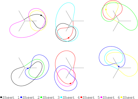
Figure 2. Homology basis in $(z,w)$ coordinates

It is now straightforward to transform this homology basis to the other coordinate systems as needed. This homology basis will be used to prove Theorem 1.

4.1. Action of symmetries on the homology basis

Having defined our homology basis and the symmetries it is a simple matter to apply one to the other and write down the action of each automorphism on the homology. It is here we have implemented code to do this. With $\gamma=\left(\mathfrak{a}_{1},\mathfrak{a}_{2},\mathfrak{a}_{3},\mathfrak{b}_{1},\mathfrak{b}_{2},\mathfrak{b}_{3}\right)^{T}$ we calculate intersection numbers to determine the matrix $M$ introduced earlier. If we are considering the automorphism $\sigma$ with $\sigma_{*}:\gamma_{i}\mapsto M_{ij}\gamma_{j},$ and $\left<\cdot,\cdot\right>$ represents the intersection number then

$$\left<\sigma_{*}(\gamma_{i}),\gamma_{k}\right>=M_{ij}\left<\gamma_{j},\gamma_{k}\right>=M_{ij}J_{jk},$$

so $M_{ij}=\left<\sigma_{*}(\gamma_{i}),\gamma_{k}\right>J_{kj}^{-1}$ which is a trivial combination of intersection numbers. The results are

• Order 3 automorphism. No computation is needed here. By definition of the homology this cyclically permutes the $A_{i}$ and $B_{i}$ independently.

  $$M=\begin{pmatrix}0&1&0&0&0&0\\ 0&0&1&0&0&0\\ 1&0&0&0&0&0\\ 0&0&0&0&1&0\\ 0&0&0&0&0&1\\ 0&0&0&1&0&0\\ \end{pmatrix}.$$

• Antiholomorphic involution.

  $$M=\begin{pmatrix}0&0&0&-1&0&0\\ 0&0&0&0&-1&0\\ 0&0&0&0&0&-1\\ -1&0&0&0&0&0\\ 0&-1&0&0&0&0\\ 0&0&-1&0&0&0\\ \end{pmatrix}.$$

• Order 7 automorphism. Although this acts simply on paths by just shifting sheets a fairly complicated matrix results.

  $$M=\begin{pmatrix}1&0&-1&1&0&-1\\ 0&0&0&0&1&0\\ -1&0&-1&0&1&0\\ -1&0&0&0&1&0\\ 0&-1&-1&1&0&0\\ 1&0&0&0&0&-1\end{pmatrix}.$$

  However, since we know that $\mathfrak{b}_{i}$ is simply $\mathfrak{a}_{i}$ shifted by some sheet number, we know that some power of this automorphism will map $\mathfrak{a}_{i}$ to $\mathfrak{b}_{i}$. Indeed $M$ itself takes $\mathfrak{a}_{2}$ to $\mathfrak{b}_{2}$; $M^{2}$ takes $\mathfrak{a}_{1}$ to $\mathfrak{b}_{1}$; and $M^{4}$ takes $\mathfrak{a}_{3}$ to $\mathfrak{b}_{3}$.

• Order 2 involution. This has a remarkably simple effect on the homology, given its complexity as a transformation.

  $$M=\begin{pmatrix}0&0&-1&0&0&0\\ 0&-1&0&0&0&0\\ -1&0&0&0&0&0\\ 0&0&0&0&0&-1\\ 0&0&0&0&-1&0\\ 0&0&0&-1&0&0\end{pmatrix}.$$

We note in passing that these matrices were produced by applying the extcurves intersection routines in the form

> find_homology_transform(curve, homSrc, homDst):

for appropriate choices of the parameters, where homSrc$=\{\mathfrak{a}_{i},\mathfrak{b_{i}}\}$ and homDst=$\{\sigma_{\ast}(\mathfrak{a}_{i}),\sigma_{\ast}(\mathfrak{b_{i}})\}$ and $\sigma$ is the automorphism being considered.

5. The period matrix

We now have the matrices $M$ and $L$ necessary to employ (2.1). We shall briefly remark on the restrictions that each symmetry results in.

5.1. Order 3 symmetry

This symmetry constrains the $\mathfrak{a}$-periods and $\mathfrak{b}$-periods separately, but in an identical manner, so we only comment on the former. Here the matrix relation is

$$\begin{pmatrix}0&1&0\\ 0&0&1\\ 1&0&0\end{pmatrix}\mathcal{A}=\mathcal{A}\begin{pmatrix}0&0&1\\ 1&0&0\\ 0&1&0\end{pmatrix},$$

which results in

$$\mathcal{A}=\begin{pmatrix}X&Y&Z\\ Y&Z&X\\ Z&X&Y\end{pmatrix}.$$

5.2. Antiholomorphic involution

This determines the $\mathfrak{b}$-periods in terms of the $\mathfrak{a}$-periods. Calling the symmetry $\sigma$, we have

$$\mathcal{B}_{ij} =\int_{\mathfrak{b}_{i}}\omega_{j}=-\int_{\sigma(\mathfrak{a}_{i})}\omega_{j}=-\int_{\mathfrak{a}_{i}}\sigma^{*}(\omega_{j})=-\int_{\mathfrak{a}_{i}}\overline{\omega}_{j}=-\overline{\int_{\mathfrak{a}_{i}}\omega_{j}}=-\overline{\mathcal{A}}_{ij}.$$

5.3. Order 7 automorphism

This symmetry sends $\mathfrak{a}_{2}$ to $\mathfrak{b}_{2}$ so it tells us

$$-\overline{Y}=\zeta^{2}Y,\qquad-\overline{Z}=\zeta Z,\qquad-\overline{X}=\zeta^{4}X.$$

This fixes the argument of all three numbers, up to sign. So if we merely constrain $r_{1},r_{2},r_{3}$ to be real then we may write

$$X =r_{1}\exp(-\pi\mathrm{i}/14), Y =r_{2}\exp(-11\pi\mathrm{i}/14), Z =r_{3}\exp(-9\pi\mathrm{i}/14)$$

(The choice has actually been made so that all $r_{i}$ are positive.)

5.4. Holomorphic involution

Here we find that

(5.1) $$-\begin{pmatrix}Z&X&Y\\ Y&Z&X\\ X&Y&Z\end{pmatrix}=\begin{pmatrix}X&Y&Z\\ Y&Z&X\\ Z&X&Y\end{pmatrix}\begin{pmatrix}\alpha&\beta&\gamma\\ \beta&\gamma&\alpha\\ \gamma&\alpha&\beta\end{pmatrix}.$$

While this naively looks like three independent equations the relations (3.4) in fact mean that there is only one independent (complex) equation in (5.1). For example, if we multiply the first equation $\alpha X+\beta Y+\gamma Z=-Z$ in (5.1) by $(\beta+1)/\alpha$ we obtain (up to rewriting) the second equation $(\beta+1)X+\gamma Y+\alpha Z=0$. Now as at this stage we only have three real parameters $r_{1},r_{2},r_{3}$ left this one complex equation is sufficient to determine (say) $r_{1}$ and $r_{2}$ in terms of $r_{3}$ and hence the matrix of periods up to an overall real multiple. Indeed, this real multiple cancels when calculating the the Riemann form of the period matrix, but as we will see in the next subsection even this scalar parameter is explicitly calculable.

Take the first entry of (5.1) as our starting point;

$$\alpha X+\beta Y+\gamma Z=-Z.$$

With $r_{1}=\mu r_{3}$, $r_{2}=\nu r_{3}$ we find a quadratic solution for $\mu,\nu$ in terms of the algebraic coefficients. Their minimal polynomials over $\mathbb{Q}$ are simply

$$\mu^{3}+\mu^{2}-2\mu-1=0,\qquad\nu^{3}-2\nu^{2}-\nu+1=0.$$

In fact each of these have three real roots, and split over $\mathbb{Q}(\zeta)$. The solution is seen to be

$$\mu=\zeta+\zeta^{-1},\qquad\nu=1+\zeta+\zeta^{-1}.$$

5.5. The final free parameter

The final free parameter can be computed most readily from the integral in the $(t,s)$ space. The cycle $\mathfrak{a}_{1}$ can be deformed to a path traversing $t=0$ to $t=1$ and then back again on a different sheet. Along this segment there is a sheet where $s$ remains real, and all other sheets are simply related by multiplication with some power of $\zeta$. Thus for example

$$Z =\int_{\mathfrak{a}_{1}}\omega_{3}=\int_{\mathfrak{a}_{1}}\frac{\mathrm{d}t}{7s^{3}}=\frac{\zeta^{k}-\zeta^{l}}{7}\int_{0}^{1}\frac{\mathrm{d}t}{s^{3}}=\frac{\zeta^{k}-\zeta^{l}}{7}\int_{0}^{1}\frac{\mathrm{d}t}{t^{3/7}(t-1)^{6/7}}=\frac{B(\frac{4}{7},\frac{1}{7})}{7}(\zeta^{k}-\zeta^{l}).$$

All that remains is to determine the integers $k$ and $l$. This is a trivial matter of analytically continuing the path $\mathfrak{a}_{1}$ over to somewhere on the segment $(0,1)$ and noting the argument of the result. We discover

$$Z=\frac{B(\frac{4}{7},\frac{1}{7})}{7}(\zeta^{-1}-1).$$

Using this to express $r_{3}$ in terms of $\Gamma$-functions rather than $B$-functions

$$r_{3}=2\sin(\pi/7)\frac{\Gamma(\frac{8}{7})\Gamma(\frac{4}{7})}{\Gamma(\frac{5}{7})}.$$

5.6. The Riemann period matrix

The Riemann period matrix is $\tau=\mathcal{B}\mathcal{A}^{-1}.$ Bringing our results together yields (1.1).

6. The relation to the period matrix of Rauch and Lewittes

6.1. Hyperbolic model of Klein’s curve

Rauch and Lewittes [RL] have already described a canonical homology basis for this curve and calculated the associated Riemann period matrix. In general finding the symplectic transformation between two period matrices is a hard problem. The best approach is usually to work with the homology bases involved and relate those.

Rauch and Lewittes’ description is based on the expression of Klein’s curve as a quotient of the hyperbolic disc, so in order to compare the two results we will need some understanding of that model.

The hyperbolic model amounts to a regular 14-gon centred in the disc, and the identification of vertices and pairs of sides around this as indicated in Figure 3. It may be tiled by 336 triangles with angles $(2\pi/7,\pi/3,\pi/2)$, each of which can form a fundamental domain of the symmetry group. This group is then manifest as rotations about any triangular vertex together with reflections in any geodesic line consisting of triangular edges.

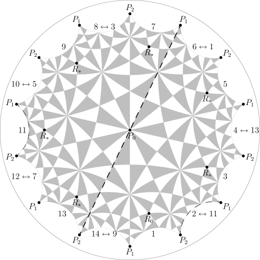
Figure 3. Hyperbolic disc model of Klein’s curve.

Rauch and Lewittes’ homology basis is described in terms of paths back and forth between $P_{1}$ and $P_{2}$ along prescribed edges. Taking positive numbers to indicate anticlockwise traversal (about the centre) and negative the reverse, the basis is explicitly

$$\mathfrak{a}^{\prime}_{1} =1-4-7-9,\qquad\mathfrak{a}^{\prime}_{2}=-4-9,\qquad\mathfrak{a}^{\prime}_{3}=-4-5,$$

$$\mathfrak{b}^{\prime}_{1} =2+3+4+5,\qquad\mathfrak{b}^{\prime}_{2}=-3+7,\qquad\mathfrak{b}^{\prime}_{3}=3-5.$$

(So for example $\mathfrak{a}^{\prime}_{1}$ consists of moving from $P_{1}$ to $P_{2}$ along side 1, back to $P_{1}$ along 7, to $P_{2}$ again along 4 and finally back to the start along 9. Although there is ambiguity in the order of edges taken all the resulting paths are homologous.)

6.2. Identification of the two models

We now wish to identify the two models of Klein’s curve so we can express Rauch and Lewittes’ homology basis in some coordinate plane. Working in $(t,s)$ coordinates we are seeking two meromorphic functions $t,s$ on the hyperbolic disc with the property that

$$s(p)^{7}=t(p)(t(p)-1)^{2}$$

everywhere. If we could describe such functions well enough then we could write down the coordinate projection of the hyperbolic basis. There is obviously no unique choice for such functions since the push-forward of any pair under an automorphism would in general give a different pair. However, we can exploit this to produce some $t,s$ with useful properties.

Consider the subgroup $H$ of the full automorphism group generated by

$$Z:(t,s) \mapsto(t,\zeta s), R:(t,s) \mapsto\left(1-\frac{1}{t},\frac{t-1}{s^{3}}\right), c:(t,s) \mapsto(\bar{t},\bar{s}).$$

These satisfy the relations $Z^{7}=R^{3}=c^{2}=1$, $RZR^{-1}=Z^{4}$, $cRc^{-1}=R$, $cZc^{-1}=Z^{-1}$ which allow us to write

$$H=\{c^{i}Z^{j}R^{k}|i=0,1;\ j=0,\ldots,6;\ k=0,1,2\},$$

and hence $H$ has 42 elements.

It is easy to verify that the full symmetry group of Klein’s curve (which is isomorphic to $PGL(2,7)$) has eight subgroups of order 42, all of which are conjugate. So if we can find an appropriate such subgroup on the hyperbolic model (one which interacts well with Rauch and Lewittes’ basis ideally) then by applying some automorphism we may assume without loss of generality that this is our group. This is helpful because, for example, the transformation $Z$ has a simple description in terms of the $s$, $t$ coordinates.

To obtain the hyperbolic group, we start with rotations of order 7 about $P_{0}$ and adjoin the rotations of order three about the indicated points $R_{\bullet}$. This in itself is a group, and has order 21 (1 identity + 6 rotations of order 7 + $7\times 2$ rotations of order 3). Let $\hat{H}$ be the result of adjoining a reflection in a diameter through $P_{1}$ to this group. It has the required 42 elements and can be made the counterpart of $H$ in the hyperbolic model.

Specifically, suppose we found an arbitrary pair of functions $t,s$ with the required algebraic relations. This induces a hyperbolic subgroup corresponding to $H$. If this is not $\hat{H}$ then they are at least conjugate so $\hat{H}=g^{-1}Hg$. But then if we instead use the meromorphic pair $t\circ g,s\circ g$ then $H$ will induce $\hat{H}$ itself. In fact, by similar means, remaining within the group $\hat{H}$ we can demand more.

We start with $c$. This fixes an entire line pointwise in $H$. The only elements of $\hat{H}$ with this property are reflections in the diametric geodesics, so $c$ must correspond to one of those. But we can do better: conjugating with some central rotation in the same way we did before we can guarantee that $c$ corresponds to the reflection that fixes edge 2 as indicated in Figure 3. Consequently we have guaranteed that the functions $s(p)$, $t(p)$ are real on edge 2.

Having made this demand, we discover that the possible images for $R$ in $\hat{H}$ are severely limited. In order to satisfy $cRc^{-1}=R$, $R$ must be some rotation about $R_{0}$ in $\hat{H}$. Finally, in order to satisfy $RZR^{-1}=Z^{4}$ we actually need $R$ to correspond to the anticlockwise rotation of $2\pi/3$ about $R_{0}$.

Now, $Z$ must correspond to one of the central rotations. So the fixed points of $Z$, namely $t=0,1,\infty$ must correspond to $P_{0},P_{1},P_{2}$ in some order. But since rotations about $R_{0}$ permute these we can conjugate again to demand that $t(P_{0})=\infty$. It is easily checked that this disrupts neither the group $\hat{H}$ nor our previous choice of $c$ (essentially because $RcR^{-1}=c^{-1}=c$). Before abandoning this issue we note that $R(\infty,\bullet)=(1,\bullet)$ and that the corresponding element of $\hat{H}$ sends $P_{0}$ to $P_{1}$ so $t(P_{1})=1$, $t(P_{2})=0$.

At this stage we know that traversing side 2 (or 11) is equivalent to travelling from $t=0$ to $t=1$ along the real axis. If we knew that $Z$ ($s\mapsto\zeta s$) corresponded to a central rotation by $2\pi j/7$ then we could deduce the phase of $s$ along any numbered edge in terms of $j$. Specifically along edge $2k$

$$s\in\zeta^{(k-1)j^{-1}}\mathbb{R},$$

where the inverse $j^{-1}$ is taken (mod 7). The odd edges are obtained by their identification with even edges. This would be enough to completely determine any path expressed, as Rauch and Lewittes do, by which numbered edges should be traversed in the hyperbolic model.

So our final task is to identify $j$ or equivalently which central hyperbolic rotation our coordinate transformation $Z$ corresponds to. The solution is provided by the hyperbolic structure near the point $P_{1}$. The idea is that $P_{1}$ is the centre of a septagon and if you go towards it on some edge and away on another then the angle between these paths corresponds to how many branch cuts you would cross doing the same thing in coordinate space. Requiring the same phase for $s$ from both processes is enough to fix $j$.

More precisely, we can deduce from Figure 3 how the numbered edges are laid out around $P_{1}$ and $P_{2}$. For example the bottom vertex shows us that an anticlockwise rotation of $2\pi/7$ about $P_{1}$ will take us from edge 1 to edge 14. Putting all this information together, we obtain Figure 4.

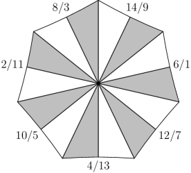
Figure 4. How edges come together near $P_{1}$

Now notice the unlabelled “spokes” in the diagram. We can think of these as branch cuts in coordinate space. If a branch cut was some ray from $t=1$ on all sheets, then in hyperbolic space these would be represented by a single line and its images under the sheet-changing operator $Z$ (or some power). These lines won’t necessarily be geodesic, but they will have a well-defined direction emerging from $P_{1}$ and be related by some $2\pi/7$ rotation in Figure 4. Thus (for example by considering a small neighbourhood around $P_{1}$) we may as well consider the unlabelled “spokes” as the branch cuts.

Now we can put these two pictures together. Suppose we start with both $t$ and $s$ real. If we go around the branch point $t=1$ once anticlockwise we discover that $s\in\zeta^{2}\mathbb{R}$. In doing so we’ve crossed just one branch cut. In the hyperbolic picture what we’ve done is start on edge 2 and go anticlockwise crossing one spoke. So we are on edge 10. But this corresponds to $s\in\zeta^{4j^{-1}}\mathbb{R}$. For these two statements to be consistent $j=2$ and $Z$ corresponds to a central rotation of $4\pi/7$ and the argument of $s$ along each edge is as in Table 2.

Edge	2/11	4/13	6/1	8/3	10/5	12/7	14/9
Phase	1	$\zeta^{4}$	$\zeta$	$\zeta^{5}$	$\zeta^{2}$	$\zeta^{6}$	$\zeta^{3}$

Table 2. $s$ phase on each numbered edge

Note that in the above there was an ambiguity over the direction of paths – an implicit assumption that anticlockwise was the same in both models. This corresponds to a choice of orientation. Group theoretically if we conjugate by $c$ it takes us between these two choices (because $cZc^{-1}=Z^{-1}$). The choice made gives us a symplectic transformation between the two homology bases, rather than antisymplectic.

6.3. Rauch and Lewittes’ Homology in Coordinates

With the above identification, we can simply read off which sheets Rauch and Lewitte’s homology basis uses in its repeated journeys between $t=0$ and $t=1$. From that information we put together paths that make the same journeys and so draw the basis. We obtain Figure 5.

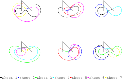
Figure 5. Rauch and Lewitte’s homology basis in $(t,s)$ coordinates.

We can algorithmically check that these paths form a canonical homology basis, and indeed we discover the correct intersection matrix.

It is now a simple matter to calculate the symplectic transformation moving from our basis to this one and the result is the previously stated (1.2). The symplectic equivalence between period matrices gives a nontrivial test of this identification.

7. Other period matrices

Tretkoff and Tretkoff [TT], Schindler [BS-a], Rodríguez and González-Aguilera [RG], Yoshida [Yo] and Tadokoro [Ta] have all described homology bases for Klein’s curve and calculated the resulting period matrices. Here we relate their works with ours, beginning with those presenting Klein’s curve as a plane projective model.

7.1. Yoshida’s period matrix

The symplectic transformation

$$\begin{pmatrix}0&0&0&-1&0&0\\ 0&1&0&0&0&-1\\ 0&0&1&0&-1&1\\ 1&1&0&0&0&-1\\ 0&1&1&-1&0&0\\ 0&1&0&0&0&0\end{pmatrix}$$

takes our period matrix to that given by Yoshida,

$$\frac{1}{14}\begin{pmatrix}6\mathrm{i}\sqrt{7}&7+3\mathrm{i}\sqrt{7}&2\mathrm{i}\sqrt{7}\\ 7+3\mathrm{i}\sqrt{7}&7+5\mathrm{i}\sqrt{7}&7+\mathrm{i}\sqrt{7}\\ 2\mathrm{i}\sqrt{7}&7+\mathrm{i}\sqrt{7}&7+3\mathrm{i}\sqrt{7}\end{pmatrix}.$$

7.2. Tadokoro’s period matrix

Similarly the symplectic transformation

$$\begin{pmatrix}0&0&0&1&0&0\\ 0&-1&1&0&-1&1\\ 0&1&0&-1&0&-1\\ -1&1&0&-1&1&0\\ 0&1&0&-1&0&0\\ 0&1&1&-1&0&0\end{pmatrix}.$$

takes our period matrix to the period matrix given by Tadokoro,

$$\frac{1}{8}\begin{pmatrix}-1+3\mathrm{i}\sqrt{7}&-3+\mathrm{i}\sqrt{7}&2+2\mathrm{i}\sqrt{7}\\ -3+\mathrm{i}\sqrt{7}&\-1+3\mathrm{i}\sqrt{7}&2+2\mathrm{i}\sqrt{7}\\ 2+2\mathrm{i}\sqrt{7}&2+2\mathrm{i}\sqrt{7}&4+4\mathrm{i}\sqrt{7}\end{pmatrix}.$$

7.3. Tretkoff and Tretkoff’s period matrix

In [TT] these authors develop the algorithm (named after them) that determines an homology basis of a Riemann surface and Klein’s curve is one of the examples given there (p495-498). This is the algorithm implemented in Maple’s algcurves. Here the author’s reproduce the work of Hurwitz, Klein and Fricke, and Baker with the choice of cycles given by those earlier works. Finally they then relate these cycles to a canonical homology basis and produce a period matrix. The symplectic transformation

$$\begin{pmatrix}0&0&-1&1&0&0\\ 0&1&1&-1&0&0\\ 0&0&-1&0&0&0\\ -1&0&-1&1&1&0\\ 0&0&0&0&1&0\\ 1&0&0&0&0&-1\end{pmatrix}.$$

takes our period matrix to

$$\frac{1}{8}\begin{pmatrix}7+3\mathrm{i}\sqrt{7}&-3+\mathrm{i}\sqrt{7}&-5-\mathrm{i}\sqrt{7}\\ -3+\mathrm{i}\sqrt{7}&-1+3\mathrm{i}\sqrt{7}&-3+\mathrm{i}\sqrt{7}\\ -5-\mathrm{i}\sqrt{7}&-3+\mathrm{i}\sqrt{7}&-1+3\mathrm{i}\sqrt{7}\end{pmatrix}.$$

This is not quite the period matrix Tretkoff and Tretkoff give. One finds that although the matrix given on the left-hand-side at the top of p498 is correct, in the final evaluation an error has been made in their $2\tau^{3}$ terms; correcting this yields the above.

7.4. Schindler’s period matrix

The period matrix of Klein’s curve was also calculated in the thesis [BS-a]. Comparing the homology bases of our works yields the following symplectic transformation

$$\begin{pmatrix}1&0&0&0&-1&0\\ 0&-1&-1&1&0&1\\ 0&-2&-1&2&0&1\\ -1&0&-1&1&1&1\\ 2&1&1&-1&-1&-3\\ -1&0&0&0&0&1\end{pmatrix}.$$

This leads to the period matrix

(7.1) $$\frac{1}{14}\begin{pmatrix}6\mathrm{i}\sqrt{7}-14&21-5\mathrm{i}\sqrt{7}&-7+3\mathrm{i}\sqrt{7}\\ 21-5\mathrm{i}\sqrt{7}&-42+10\mathrm{i}\sqrt{7}&14-6\mathrm{i}\sqrt{7}\\ -7+3\mathrm{i}\sqrt{7}&14-6\mathrm{i}\sqrt{7}&-7+5\mathrm{i}\sqrt{7}\end{pmatrix}.$$

Here we find that the imaginary parts of this and Schindler’s period matrix agree but the real parts are in disagreement. We believe a typographic error before the final substitution led to an incorrect result. The result (7.1) should replace that given in [BL, Exercise 11.15] (the imaginary parts of these agree however).

7.5. The Rodríguez and González-Aguilera period matrix

These authors consider the classically studied KFT pencil of curves

$$x^{4}+y^{4}+z^{4}+t(x^{2}y^{2}+y^{2}z^{2}+z^{2}x^{2})=0$$

in terms of a hyperbolic model. For $t=-3(1\pm\mathrm{i}\sqrt{7})/2$ this is Klein’s curve, for $t=0$ this is Fermat’s quartic curve, and for $t=-2$ the tetrahedron, and so the nomenclature. There are various singular fibres in this pencil. Away from these the period matrix takes the form

$$\tau(t)\begin{pmatrix}3&-1&-1\\ -1&3&-1\\ -1&-1&3\end{pmatrix}$$

and the Jacobian is isogenous to the product of three elliptic curves. Klein’s curve corresponds to $\tau(t)=(5+\mathrm{i}\sqrt{7})/2$ and the symplectic transformation

$$\begin{pmatrix}0&0&1&-1&0&0\\ 0&1&1&-1&0&0\\ 0&0&1&0&0&0\\ 1&-1&1&-1&-1&0\\ 0&2&0&-1&1&0\\ -1&-1&1&1&0&1\end{pmatrix}.$$

takes our period matrix to this.

References

- [BBM] M, B. Babich, A. I. Bobenko and V. B. Matveev, Reductions of Riemann theta functions of genus to theta functions of lesser genus, and symmetries of algebraic curves, Dokl. Akad. Nauk SSSR 272 (1983), no. 1, 13–17.
- [Ba] H.F. Baker, Multiply Periodic Functions, Cambridge University Press, Cambridge, 1907.
- [BL] Christina Birkenhake and Herbert Lange, Complex Abelian Varieties Second edition, Springer-Verlag, Berlin 2004.
- [Bo] Oskar Bolza, On Binary Sextics with Linear Transformations into Themselves, Amer. J. Math. 10 (1887), no. 1, 47–70.
- [BE07] H. W. Braden and V. Z. Enolski, Monopoles, Curves and Ramanujan, To be published. arXiv: math-ph/0704.3939.
- [BE09] by same author, On the tetrahedrally symmetric monopole, arXiv: math-ph/0908.3449
- [B] H. W. Braden, Cyclic Monopoles, Affine Toda and Spectral Curves, arXiv:1002.1216
- [BK] Integrability: the Seiberg-Witten and Whitham equations, H. W. Braden and I. M. Krichever (Eds.), Gordon and Breach Science Publishers, Amsterdam, 2000. ISBN: 90-5699-281-3.
- [BS] Peter Buser and Robert Silhol, Geodesics, Periods and Equations of Real Hyperelliptic Curves, Duke Math. J. 108 (2001) 211–244.
- [D] A. D’Avanzo, On Charge 3 Cyclic monopoles, Edinburgh Ph.D. Thesis, 2010.
- [FK] Robert Fricke and Felix Klein, Vorlesungen ber die Theorie der automorphen Funktionen. Band II: Die funktionentheoretischen Ausf hrungen und die Andwendungen Teubner, Stuttgart 1912.
- [G] Jane Gilman, Canonical symplectic representations for prime order conjugacy classes of the mapping-class group, J. Algebra 318 (2007) 430–455.
- [HMM95] N. J. Hitchin, N. S. Manton and M. K. Murray, Symmetric monopoles, Nonlinearity 8 (1995), 661–692.
- [H] Adolf Hurwitz, Ueber einige besondere homogene lineare Differentialgleichungen, Math. Ann. 26 (1886), no. 1, 117–126.
- [L] Silvio Levy (Editor), The Eightfold Way: The Beauty of Klein’s Quartic Curve, Math. Sci. Research Inst. Publications.
- [RL] Harry E. Rauch and J. Lewittes, The Riemann surface of Klein with 168 automorphisms, Problems in analysis (papers dedicated to Salomon Bochner, 1969), pp. 297–308. Princeton Univ. Press, Princeton, N.J., 1970.
- [RR] Gonzalo Riera and Rubí E Rodriguez, The period matrix of Bring’s curve, Pacific J. Math. 154 (1992), no. 1, 179–200.
- [RG] Rubí E Rodríguez and Víctor González-Aguilera, Fermat’s quartic curve, Klein’s curve and the tetrahedron, in Extremal Riemann surfaces (San Francisco, CA, 1995), 43–62, Contemp. Math., 201, Amer. Math. Soc., Providence, RI, 1997.
- [JS-a] John Schiller, Riemann matrices for hyperelliptic surfaces with involutions other than the interchange of sheets, Michigan Math. J. 15 (1968) 283–287.
- [JS-b] John Schiller, Moduli for special Riemann surfaces of genus , Trans. Amer. Math. Soc. 144 (1969) 95–113.
- [BS-a] Bernhard Schindler, Jacobische Varietaeten hyperelliptischer Kurven und einiger spezieller Kurven vom Geschelcht 3. (Dissertation Erlangen 1991).
- [BS-b] Bernhard Schindler, Period matrices of hyperelliptic curves, Manuscripta Math. 78 (1993), no. 4, 369–380.
- [St] M. Streit, Period matrices and representation theory, Abh. Math. Sem. Univ. Hamburg 71 (2001), 279–290.
- [Ta] Yuuki Tadokoro, A nontrivial algebraic cycle in the Jacobian variety of the Klein quartic, Math. Z. 260 (2008), no. 2, 265–275.
- [TT] C. L. Tretkoff and M. D. Tretkoff, Combinatorial group theory, Riemann surfaces and differential equations, Contributions to group theory, 467–519, Contemp. Math., 33, Amer. Math. Soc., Providence, RI, 1984.
- [Yo] Katsuaki Yoshida, Klein’s surface of genus three and associated theta constants,Tsukuba J. Math. 23 (1999), no. 2, 383–416.