Photovoltaic Berry curvature in the honeycomb lattice

Abstract

Photovoltaic Hall effect — the Hall effect induced by intense, circularly-polarized light in the absence of static magnetic fields — has been proposed in Phys. Rev. B 79, 081406R (2009) for graphene where a massless Dirac dispersion is realized. The photovoltaic Berry curvature (a nonequilibrium extension of the standard Berry curvature) is the key quantity to understand this effect, which appears in the Kubo formula extended to Hall transport in the presence of strong AC field backgrounds. Here we elaborate the properties of the photovoltaic curvature such as the frequency and field strength dependence in the honeycomb lattice.

1 Introduction

Non-linear effects in electronic systems are an interesting playground to look for novel transport properties that cannot occur in equilibrium. A famous example is the Franz-Keldysh effect in semiconductors, where the band edge exhibits red-shifts in static or AC electric fields. This can be considered as an effect of the deformation of the electron wavefunction, i.e., leakage to the gap region, in strong electric fields, which leads to the change in response properties.

Recently, a novel, optically controlled non-linear phenomenon has been proposed in ref. [1], in which the present authors revealed a new type of Hall effect — photovoltaic Hall effect — can emerge in honeycomb lattices such as graphene subject to intense, circularly-polarized light despite the absence of static magnetic fields. If we denote the gauge field representing the circularly-polarized light as $\mbox{\boldmath$A$}_{\rm ac}(t)=\frac{F}{\Omega}(\cos\Omega t,\sin\Omega t)$, where $F=eE$ is the field strength and $\Omega$ the frequency of the light, the tight-binding Hamiltonian for electrons reads

$$H(t)=-\sum_{ij}t_{ij}e^{-i\hat{e}_{ij}\cdot{\bf A}_{\rm ac}(t)}c_{i}^{\dagger}c_{j},$$ (1)

where $t_{ij}=w$ is the nearest-neighbor hopping for the honeycomb lattice, $\hat{e}_{ij}$ the unit vector connecting the bond between $i$ and $j$, and spins are ignored. The Hamiltonian is time periodic, and, in momentum space the $k$-points are driven in the Brillouin zone by the field as $\mbox{\boldmath$k$}(t)=\mbox{\boldmath$k$}-\mbox{\boldmath$A$}_{\rm ac}(t)$. The orbit is a circle centered at $k$ with a radius $F/\Omega$, and the time period is $T=2\pi/\Omega$ (Fig. 1).

During the motion, the electron wave function acquires a nontrivial geometric phase, known as the Aharnov-Anandan phase[2] which is the non-adiabatic extension of the Berry phase[4] and reduces to the Berry phase in the adiabatic limit $\Omega\to 0$ with a fixed $F/\Omega$. An important feature in the electron wavefunctions in time-periodic systems, which is a temporal analogue of Bloch’s theorem for spatially periodic systems, is that the solution $|\Psi_{\alpha}(t)\rangle$ of the time-dependent Schrödinger equation can be described by the time-periodic Floquet states $|\Phi_{\alpha}(t)\rangle$ as $|\Psi_{\alpha}(t)\rangle=e^{-i\varepsilon_{\alpha}t}|\Phi_{\alpha}(t)\rangle$, where $\varepsilon_{\alpha}$ is the Floquet quasi-energy and $\alpha$ an index that labels the Floquet states. Note that $\alpha$ becomes a composite index $\alpha=(i,m)$ when the original system has an internal degrees of freedom $i$, e.g. the band index for multiband systems such as the Dirac cone with electron and hole branches, while $m=0,\pm 1,\pm 2,\ldots$ denotes the number of absorbed photons.

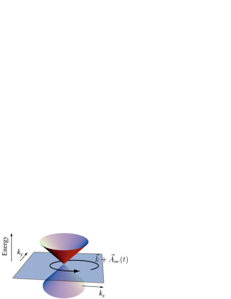
Figure 1: A trajectory of $\mbox{\boldmath$k$}+\mbox{\boldmath$A$}_{\rm ac}(t)$ around a Dirac point in a circularly-polarized light field.

The applied intense laser induces nontrivial photovoltaic transports as follows: Note first that we have two external fields, the intense laser irradiation and (ii) a weak, dc electric field for measuring the Hall effect. If we define the inner product averaged over a period of the ac laser field by $\langle\langle\alpha|\beta\rangle\rangle\equiv\frac{1}{T}\int_{0}^{T}dt\langle\alpha(t)|\beta(t)\rangle$, the Floquet states span a complete orthogonal basis in the presence of a strong laser field, and one can perform a perturbation expansion in the small dc field to probe the (Hall) conductivity to obtain a Kubo formula extended to the case of strong ac irradiation [1],

$$\sigma_{ab}(\mbox{\boldmath$A$}_{ac})=i\int\frac{d\mbox{\boldmath$k$}}{(2\pi)^{d}}\sum_{\alpha,\beta\neq\alpha}\frac{[f_{\beta}(\mbox{\boldmath$k$})-f_{\alpha}(\mbox{\boldmath$k$})]}{\varepsilon_{\beta}(\mbox{\boldmath$k$})-\varepsilon_{\alpha}(\mbox{\boldmath$k$})}\frac{\langle\langle\Phi_{\alpha}(\mbox{\boldmath$k$})|J_{b}|\Phi_{\beta}(\mbox{\boldmath$k$})\rangle\rangle\langle\langle\Phi_{\beta}(\mbox{\boldmath$k$})|J_{a}|\Phi_{\alpha}(\mbox{\boldmath$k$})\rangle\rangle}{\varepsilon_{\beta}(\mbox{\boldmath$k$})-\varepsilon_{\alpha}(\mbox{\boldmath$k$})+i\eta},$$ (2)

where $f_{\alpha}(\mbox{\boldmath$k$})$ is the non-equilibrium distribution (occupation fraction) of the $\alpha$-th Floquet state, $J$ the current operator, and $\eta$ a positive infinitesimal. The difference from the conventional Kubo formula in the absence of AC fields is that the energy is replaced with the Floquet quasi-energy, and the inner product with a time average. The photovoltaic Hall conductivity can be further simplified to [1],

$$\sigma_{xy}(\mbox{\boldmath$A$}_{\rm ac})=e^{2}\int\frac{d\mbox{\boldmath$k$}}{(2\pi)^{d}}\sum_{\alpha}f_{\alpha}(\mbox{\boldmath$k$})\left[\nabla_{\mbox{\boldmath$k$}}\times\mbox{\boldmath$\mathcal{A}$}_{\alpha}(\mbox{\boldmath$k$})\right]_{z},$$ (3)

in terms of a gauge field $\mbox{\boldmath$\mathcal{A}$}_{\alpha}(\mbox{\boldmath$k$})\equiv-i\langle\langle\Phi_{\alpha}(\mbox{\boldmath$k$})|\nabla_{\mbox{\boldmath$k$}}|\Phi_{\alpha}(\mbox{\boldmath$k$})\rangle\rangle$. This reduces to the TKNN formula [3] in the adiabatic limit. Note that the photovoltaic Hall effect does not take place in a linearly polarized light [5] which does not break the time-reversal symmetry.

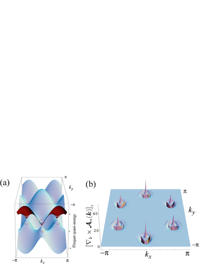
Figure 2: (a) The Floquet quasi-energy $\varepsilon$ against the wave number, and (b) the photovoltaic Berry curvature $\left[\nabla_{k}\times\mbox{\boldmath$\mathcal{A}$}_{\alpha}(\mbox{\boldmath$k$})\right]_{z}$ for the upper band for $F=0.1w,\;\Omega=1.0w$ in the honeycomb lattice.

2 Photovoltaic Berry curvature in the honeycomb lattice

Let us have a closer look at the Floquet states and the photovoltaic curvature $\left[\nabla_{\mbox{\boldmath$k$}}\times\mbox{\boldmath$\mathcal{A}$}_{\alpha}(\mbox{\boldmath$k$})\right]_{z}$ in the honeycomb lattice. We begin by noting that there exists infinite array of photo-dressed states in the Floquet spectrum, whose quasi-energy is shifted by $m\Omega$ ($m=0,\pm 1,\ldots$) from the plotted ones. In Fig. 2 (a), we plot the Floquet quasi-energy against wave number for the Floquet states having the largest weight of the $m=0$ Floquet state (a descendant of the original $F=0$ dispersion). An important feature in the plot is that the band-gap-like structure around $\varepsilon\sim\pm\Omega/2$, where the gap opens an outcome of the photo-induced hybridization of levels, a first-order effect in $F$. More importantly, a small gap opens [1] at the Dirac points around $\varepsilon\sim 0$, which is a consequence of circularly-polarized light.

The photovoltaic Berry curvature is plotted in Fig. 2 (b) for the same parameters. Around each K-point we find a peak surrounded by concentric circles and lines. The peak is due to the gap opening at the Dirac points, we can see that the sign is the same for both $K$ and $K^{\prime}$ points. They contribute equally to the photovoltaic Hall coefficient in the momentum integral in eqn. (3) and no cancellation between $K$ and $K^{\prime}$ points occurs. On the other hand, the concentric circles and lines are due to the photo-induced hybridization, e.g., the former corresponds to the band structure around $\varepsilon\sim\pm\Omega/2$ in Fig. 2 (a).

3 Experimental feasibility

The two major candidates for the observation of the photovoltaic Hall effect are

• Graphene, including multi-layer systems,

• Surface states in topological insulators,

in which Dirac-like dispersions are realized. As for the experimental feasibility, a typical intensity of laser conceived here, $F\sim 0.001w$, corresponds to $E\sim 10^{7}\mbox{V/m}$ for photon energy $\Omega\sim 1\mbox{eV}$, $w=2.7\mbox{eV},\;a=2.6\AA$. The size of the photovoltaic Dirac gap $\Delta=2\kappa$ scales as

$$\Delta\propto F^{2}/\Omega^{3}$$ (4)

for small field strengths, which was derived in ref. [1]. This formula implies that with a smaller laser energy $\Omega$ we can realize the photovoltaic Hall effect with a weaker laser strength $F$. Hence it should be interesting to study the $\Omega$ dependence of the photovoltaic Hall effect. Another important point is that in graphene, the Dirac dispersion is realized near zero energy, but the dispersion begins to reflect the lattice structure for higher energies, hence for higher values of $\Omega$. So we may ask: Will the Hall effect survive when $\Omega$ becomes large, say comparable with the band width?

In order to clarify this point, we have calculated the photovoltaic Berry curvature for several values of $\Omega$ in Fig. 3. For a smaller frequency in Fig. 3 (a), the central peak becomes smaller and broader. The surrounding concentric circles become closely packed and increase in number because we now have contributions from photo-induced hybridization around $\varepsilon\sim\pm\Omega$ in addition to $\varepsilon\sim\pm\Omega/2$. For a larger frequency in Fig. 3 (b), on the other hand, the peaks survive even though $\Omega$ is greater than the band width. However, the peak becomes smaller (and narrower), so it will become more difficult to observe the effect.

In Fig. 3 (c), we plot the Photovoltaic Hall coefficient (eqn.(3)) against the strength of the circularly polarized light. Here, we assumed sudden switch on of the electric fields, which implies $f_{\alpha}=\sum_{E_{n}<E_{F}}|\langle\langle\Phi_{\alpha}|\psi_{n}\rangle\rangle|^{2}$, where $|\psi_{n}\rangle$ is the zero field eigen-wavefunction, and $E_{n}$ its energy. This assumption is expected to breakdown in the presence of dissipation, however, the basic trend do not change which was confirmed by calculations based on more elaborate techniques [1]. As expected from the scaling relation of the photovoltaic Dirac gap $\Delta$ (eqn. (4)), the Hall coefficient first increases as $\mbox{Re}~{}\sigma_{xy}\propto\Delta\propto F^{2}/\Omega^{3}$ in the weak field limit. At this field strength, the physics can be understood by the central peaks of the Berry curvature at the K and K’ points. However, after saturating at a certain value, the Hall coefficient starts to decrease and become negative. When this happens, the electrons are deeply in the ac-Wannier Stark ladder regime and are localized due to the strong circularly polarized light. The Berry curvature peaks around the K and K’ points now become highly complex and the sign alters at each concentric circles as shown in Fig. 3 (a). This leads to negative Hall coefficients after integrating over the Brillouin Zone.

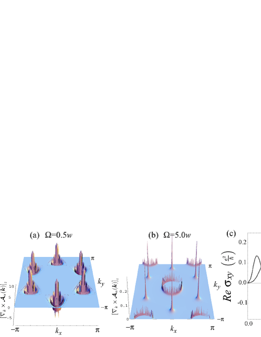
Figure 3: Photovoltaic Berry curvature for (a) $\Omega=0.5w$ and (b) $\Omega=5.0w$ with the same field strength as Fig. 2. (c) The dependence of the Photovoltaic Hall coefficient $\mbox{Re}~{}\sigma_{xy}$ on the strength of the ac-electric field $F$ in the honeycomb lattice.

4 Conclusion

We have studied the dependence of the photovoltaic Hall effect in a honeycomb lattice. Especially, we have elaborated the dependence of the photovoltaic Berry curvature on the frequency $\Omega$ of the applied circularly-polarized light. We have found that the photovoltaic Berry curvature and thus, the Hall coefficient gradually increases as $\Omega$ becomes smaller reflecting the relation $\mbox{Re}~{}\sigma_{xy}\propto\Delta\propto F^{2}/\Omega^{3}$. However, even when $\Omega$ is large and the Dirac band approximation breaks down, we found evidence that the photovoltaic Hall effect survives, which indicates that this is not limited to Dirac bands but the effect is more universal and can be realized in a wide range of electron systems in circularly polarized light.

TO was supported by Grant-in-Aid for young Scientists (B).

References

References

- [1] T. Oka and H. Aoki, Phys. Rev. B 79, 081406R (2009), Erratam: ibid. 79, 169901 (2009).
- [2] Y. Aharonov and J. Anandan, Phys. Rev. Lett. 58, 1593 (1987).
- [3] D. J. Thouless, et al., Phys. Rev. Lett. 49, 405 (1982).
- [4] M. V. Berry, Proc. R. Soc. Lond. A 392, 45 (1984).
- [5] S. V. Syzranov, et al., Phys. Rev. B 78, 045407 (2008).