Non-existence of stationary two-black-hole configurations

Abstract

We resume former discussions of the question, whether the spin-spin repulsion and the gravitational attraction of two aligned black holes can balance each other. To answer the question we formulate a boundary value problem for two separate (Killing-) horizons and apply the inverse (scattering) method to solve it. Making use of results of Manko, Ruiz and Sanabria-Gómez and a novel black hole criterion, we prove the non-existence of the equilibrium situation in question.

1 Introduction

This paper is meant to contribute to the present discussion about the existence or non-existence of stationary equilibrium configurations consisting of separate bodies at rest. Hermann Weyl, whom Jürgen Ehlers admired especially, was the first person to consider the problem of two separate static (axisymmetric) bodies in equilibrium Weyl . To mention only one modern advancement in this field we refer to a paper by Beig and Schoen Beig , who were able to prove a non-existence theorem for a reflectionally symmetric static $n$-body configuration.

Our intention is to involve the interaction of the angular momenta of rotating bodies (“spin-spin interaction”) which could generate repulsive effects compensating the omnipresent mass attraction. A characteristic example for such a stationary configuration could be the equilibrium between two aligned rotating black holes. We will present and review a chain of old and new arguments which finally forbid the equilibrium situation.

Our argumentation is based on a boundary value problem for two separate (Killing-) horizons (see Fig. 1) and the characterization of sub-extremal black holes by Booth and Fairhurst Booth and follows the ideas of Manko and Ruiz Manko2001 who solved the equilibrium problem for the so-called double-Kerr solution.

Figure 1: Illustration of the two-black-hole equilibrium situation in Weyl coordinates. The event horizons $\mathcal{H}_{1}$ and $\mathcal{H}_{2}$ of the two black holes are located in the intervals $[K_{2},K_{1}]$ and $[K_{4},K_{3}]$ on the $\zeta$-axis, respectively. The remaining parts $\mathcal{A}^{\pm}$, $\mathcal{A}^{0}$ of the $\zeta$-axis correspond to the rotation axis.

The double-Kerr (more precicely: double-Kerr-NUT) solution, first derived in Neugebauer1980a ; Kramer1980 , is a seven parameter solution constructed by a two-fold Bäcklund transformation of Minkowski space. Since a single Bäcklund transformation generates the Kerr-NUT solution that contains, by a special choice of its three parameters, the stationary black hole solution (Kerr solution) and since Bäcklund transformations act as a “nonlinear” superposition principle, the double-Kerr-NUT solution was considered to be a good candidate for the solution of the two horizon problem and extensively discussed in the literature Kramer1980 ; Kihara1982 ; Tomimatsu ; Hoenselaers1983 ; Yamazaki ; Hoenselaers1984 ; Dietz ; Kramer1986 ; Manko2000 ; Krenzer ; Manko2001 . However, there was no argument requiring that this particular solution be the only candidate. In this paper we will remove this objection and show that the discussion of a boundary value problem for two separate horizons necessarily leads to the double-Kerr-NUT solution. Thus we can make use of the equilibrium conditions for this solution which ensure that the intervals $\mathcal{A}^{+}$, $\mathcal{A}^{0}$, $\mathcal{A}^{-}$ (see Fig. 1) are regular parts of the axis of symmetry. After a too restrictive ansatz in Kramer1980 , Tomimatsu and Kihara Kihara1982 ; Tomimatsu derived and discussed a complete set of equilibrium conditions on the axis. Reformulations and numerical studies by Hoenselaers Hoenselaers1984 made plausible that the two gravitational sources (black hole candidates) of the double-Kerr-NUT solution (located at the intervals $\varrho=0$, $K_{1}\geq\zeta\geq K_{2}$ and $K_{3}\geq\zeta\geq K_{4}$) cannot be in equilibrium if their Komar masses are positive. The first decisive step toward prove the Hoenselaers conjecture was taken by Manko, Ruiz and Sanabria-Gómez Manko2000 , who derived an explicit and easily applicable form of the Tomimatsu-Kihara equilibrium conditions and, as an important complement, analytical formulae for the Komar masses and angular momenta of the gravitational sources. Manko and Ruiz Manko2001 completed their non-existence proof by showing that the equilibrium conditions for the double-Kerr-NUT solution are indeed violated for positive Komar masses. This is, however, a critical point of their analysis. To the best of our knowledge there is no argument in favour of the positiveness of the Komar mass. (On the contrary, Ansorg and Petroff Ansorg2006 have given a convincing counterexample.)

In this paper we replace the Komar mass inequality (positivity of the Komar mass of each black hole) by an inequality connecting angular momentum and horizon area Hennig2008a . This relation is based on the causal structure of trapped surfaces in the interior vicinity of the event horizon Booth . In this way we can complete the no-go theorem, avoiding more laborious investigations of the domain outside the horizons and off the axis of symmetry (e.g., the search for singular rings or other singularities — in Sec. 5.2 we will return to that question).

2 The boundary value problem

2.1 The boundary conditions

The exterior vacuum gravitational field of axisymmetric and stationary gravitational sources can be described in cylindrical Weyl-Lewis-Papapetrou coordinates by the line element

$$\mathrm{d}s^{2}=\mathrm{e}^{-2U}\big{[}\mathrm{e}^{2k}(\mathrm{d}\varrho^{2}+\mathrm{d}\zeta^{2})+\varrho^{2}\mathrm{d}\varphi^{2}\big{]}-\mathrm{e}^{2U}(\mathrm{d}t+a\mathrm{d}\varphi)^{2},$$ (1)

where the “Newtonian” gravitational potential $U$, the “gravitomagnetic” potential $a$ and the “superpotential” $k$ are functions of $\varrho$ and $\zeta$ alone. Figure 1 shows the boundaries of the vacuum region: $\mathcal{A}^{+}$, $\mathcal{A}^{0}$, $\mathcal{A}^{-}$ are the regular parts of the axis of symmetry, $\mathcal{H}_{1}$ and $\mathcal{H}_{2}$ are Killing horizons and $\mathcal{C}$ stands for spatial infinity. Regularity of the metric along $\mathcal{A}^{+}$, $\mathcal{A}^{0}$, $\mathcal{A}^{-}$ means elementary flatness and uniqueness on the axis of symmetry,

$$\mathcal{A}^{\pm},\mathcal{A}^{0}:\quad a=0,\quad k=0.$$ (2)

The spacetime has to be flat at large distances from the horizons,

$$\mathcal{C}:\quad U\to 0,\quad a\to 0,\quad k\to 0,$$ (3)

i.e. the line element (1) takes a Minkowskian form in cylindrical space ($\varrho,\zeta,\varphi$)- time ($t$) coordinates.

The metric (1) allows an Abelian group of motions $G_{2}$ with the generators (Killing vectors)

$$\xi^{i}=\delta^{i}_{t},\quad\,\,\,\,\xi^{i}\xi_{i}<0\quad\textrm{(stationarity)},$$ (4)

$$\eta^{i}=\delta^{i}_{\varphi},\quad\eta^{i}\eta_{i}>0\quad\textrm{(axisymmetry)},$$ (5)

where the Kronecker symbols $\delta^{i}_{t}$ and $\delta^{i}_{\varphi}$ indicate that $\xi^{i}$ has only a $t$-component whereas $\eta^{i}$ points in the azimuthal $\varphi$-direction along closed circles. Obviously,

$$\mathrm{e}^{2U}=-\xi^{i}\xi_{i},\qquad a=-\mathrm{e}^{-2U}\eta_{i}\xi^{i}$$ (6)

is a coordinate-free representation of the two relativistic gravitational potentials $U$ and $a$ with the boundary values (2), (3).

In stationary and axisymmetric spacetimes, the event horizon of a black hole is a Killing horizon which can be defined by a linear combination $L$ of $\xi$ and $\eta$,

$$L=\xi+\Omega\eta,$$ (7)

where $\Omega$ is a constant. A connected component of the set of points with $\mathrm{e}^{2V}:=-(L,L)=0$, which is a null hypersurface, $(\mathrm{d}\mathrm{e}^{2V},\mathrm{d}\mathrm{e}^{2V})=0$, is called a Killing horizon $\mathcal{H}(L)$,

$$\mathcal{H}(L):\quad\mathrm{e}^{2V}=-(L,L)=0,\qquad(\mathrm{d}\mathrm{e}^{2V},\mathrm{d}\mathrm{e}^{2V})=0.$$ (8)

Since the Lie derivative $\mathcal{L}_{L}$ of $\mathrm{e}^{2V}$ vanishes, we have $(L,\mathrm{d}\mathrm{e}^{2V})=0$. Hence, $L$ and $\mathrm{e}^{2V}$ being null vectors on $\mathcal{H}(L)$ are proportional to each other,

$$\mathcal{H}(L):\quad\mathrm{d}\mathrm{e}^{2V}=-2\kappa L.$$ (9)

Using the field equations one can show that the surface gravity $\kappa$ is a constant on $\mathcal{H}(L)$. In Weyl-Lewis-Papapetrou coordinates the event horizon degenerates to a “straight line” and covers a $\zeta$-interval at $\varrho=0$ Carter . To formulate boundary conditions on the horizons $\mathcal{H}_{1}$ and $\mathcal{H}_{2}$ (see Fig. 1) we make use of (6) and (7) to express $\mathrm{e}^{2V}$ in terms of $\mathrm{e}^{2U}$, $a$ and $\varrho$,

$$\mathcal{H}_{1}:\quad\mathrm{e}^{2V_{1}}:=\mathrm{e}^{2U}\left[(1+\Omega_{1}a)^{2}-\Omega_{1}^{2}\varrho^{2}\mathrm{e}^{-4U}\right]=0,\quad\varrho=0,\quad K_{1}\geq\zeta\geq K_{2},$$ (10)

$$\mathcal{H}_{2}:\quad\mathrm{e}^{2V_{2}}:=\mathrm{e}^{2U}\left[(1+\Omega_{2}a)^{2}-\Omega_{2}^{2}\varrho^{2}\mathrm{e}^{-4U}\right]=0,\quad\varrho=0,\quad K_{3}\geq\zeta\geq K_{4}.$$ (11)

$\Omega_{1}$, $\Omega_{2}$ are the constant angular velocities of the horizons $\mathcal{H}_{1}$, $\mathcal{H}_{2}$, respectively.

2.2 The field equations

The vacuum Einstein equations for the metric potentials $U$, $a$, $k$ are equivalent to the Ernst equation

$$(\Re f)\Big{(}f_{,\varrho\varrho}+f_{,\zeta\zeta}+\frac{1}{\varrho}f_{,\varrho}\Big{)}=f_{,\varrho}^{2}+f_{,\zeta}^{2}$$ (12)

for the complex function

$$f(\varrho,\zeta)=\mathrm{e}^{2U(\varrho,\zeta)}+\mathrm{i}b(\varrho,\zeta),$$ (13)

where $b$ replaces $a$ via

$$a_{,\varrho}=\varrho\mathrm{e}^{-4U}b_{,\zeta},\qquad a_{,\zeta}=-\varrho\mathrm{e}^{-4U}b_{,\varrho}$$ (14)

and $k$ can be calculated from

$$k_{,\varrho} = \varrho\Big{[}U_{,\varrho}^{2}-U_{,\zeta}^{2}+\frac{1}{4}\mathrm{e}^{-4U}(b_{,\varrho}^{2}-b_{,\zeta}^{2})\Big{]},$$ (15)

$$k_{,\zeta} = 2\varrho\Big{[}U_{,\varrho}U_{,\zeta}+\frac{1}{4}\mathrm{e}^{-4U}b_{,\varrho}b_{,\zeta}\Big{]}.$$ (16)

As a consequence of the Ernst equation (12), the integrability conditions $a_{,\varrho\zeta}=a_{,\zeta\varrho}$ and $k_{,\varrho\zeta}=k_{,\zeta\varrho}$ are satisfied such that the metric potentials $a$ and $k$ may be calculated via line integration from the Ernst potential $f$. Thus the boundary value problem for the vacuum Einstein equations reduces to a boundary value problem for the Ernst equation. However, we have to cope with non-local boundary conditions for the Ernst potential, see (2), (3), (14), (15), (16). Fortunately, these boundary conditions are well-adapted to the “inverse method”, which will be applied to solve the boundary value problem.

2.3 The inverse method

The inverse (scattering) method first applied to solve initial value problems of special classes of non-linear partial differential equations in many areas of physics (Korteweg-de Vries equation in hydrodynamics, non-linear Schrödinger equation in non-linear optics etc.) is based on the existence of a linear problem (LP) whose integrability condition is equivalent to the non-linear differential equation. Luckily, the Ernst equation has an LP too, so one can try to tackle boundary value problems for rotating objects including black holes. We use the LP Neugebauer1979 ; Neugebauer1980b

$${\mathbold\Phi}_{,z} =\left[\left(\begin{array}[]{cc}B&0\\ 0&A\end{array}\right)+\lambda\left(\begin{array}[]{cc}0&B\\ A&0\end{array}\right)\right]{\mathbold\Phi},$$ (17)

$${\mathbold\Phi}_{,\bar{z}} =\left[\left(\begin{array}[]{cc}\bar{A}&0\\ 0&\bar{B}\end{array}\right)+\frac{1}{\lambda}\left(\begin{array}[]{cc}0&\bar{A}\\ \bar{B}&0\end{array}\right)\right]{\mathbold\Phi},$$

where ${\mathbold\Phi}(z,\bar{z},\lambda)$ is a $2\times 2$ matrix depending on the spectral parameter

$$\lambda=\sqrt{\frac{K-\mathrm{i}\bar{z}}{K+\mathrm{i}z}}$$ (18)

as well as on the complex coordinates $z=\varrho+\mathrm{i}\zeta$, $\bar{z}=\varrho-\mathrm{i}\zeta$, whereas

$$A=\frac{f_{,z}}{f+\bar{f}},\qquad B=\frac{\bar{f}_{,z}}{f+\bar{f}}$$ (19)

and the complex conjugate quantities $\bar{A}$, $\bar{B}$ are functions of $z$, $\bar{z}$ (or $\varrho$, $\zeta$) alone and do not depend on the constant parameter $K$. From the integrability condition ${\mathbold\Phi}_{,z\bar{z}}={\mathbold\Phi}_{,\bar{z}z}$ and the relations

$$\lambda_{,z}=\frac{\lambda}{4\varrho}(\lambda^{2}-1),\qquad\lambda_{,\bar{z}}=\frac{1}{4\varrho\lambda}(\lambda^{2}-1)$$ (20)

it follows that the $\lambda$-independent coefficients of a matrix polynomial in $\lambda$ have to vanish. The result is the Ernst equation (12). Vice versa, the matrix ${\mathbold\Phi}$ calculated from (17) does not depend on the path of integration if $f$ is a solution to the Ernst equation. The idea of the inverse (scattering) method is to construct ${\mathbold\Phi}$, for fixed but arbitrary values of $z$, $\bar{z}$, as a holomorphic function of $\lambda$ and to calculate $f(\varrho,\zeta)$ from ${\mathbold\Phi}$. To obtain the dependence on $\lambda$ for the two-horizon problem we have to integrate the linear system (17) along the dashed line $\mathcal{D}=\mathcal{A}^{-}\cup\mathcal{H}_{2}\cup\mathcal{A}^{0}\cup\mathcal{H}_{1}\cup\mathcal{A}^{+}\cup\mathcal{C}$ making use of the boundary conditions (2), (3), (10), (11). As was shown in Neugebauer2000 and Neugebauer2003 (see Eqs. (34), (45), (57), (58) in Neugebauer2003 ) the result of the integration is a matrix representation of the axis values of the Ernst potential $f^{+}(\zeta)\equiv f^{+}(\varrho=0,\zeta)=\mathrm{e}^{2U^{+}(\zeta)}+\mathrm{i}b^{+}(\zeta)$ on $\mathcal{A}^{+}$ in terms of the parameters $K_{i}$ ($i=1,\dots,4$), $f_{i}=f(\varrho=0,\zeta=K_{i})$ and the angular velocities $\Omega_{1}=\Omega^{(1)}=\Omega^{(2)}$, $\Omega_{2}=\Omega^{(3)}=\Omega^{(4)}$:

$$\mathcal{N}=\prod\limits_{n=1}^{4}\left({\bf 1}+\frac{{\bf F}_{n}}{2\mathrm{i}\Omega^{(n)}(\zeta-K_{n})}\right),$$ (21)

where

$$\mathcal{N}:=\mathrm{e}^{-2U^{+}(\zeta)}\left(\begin{array}[]{cc}1&-\mathrm{i}b^{+}(\zeta)\\[4.30554pt] \mathrm{i}b^{+}(\zeta)&\ f^{+}(\zeta)\bar{f}^{+}(\zeta)\end{array}\right)$$ (22)

and

$${\bf F}_{n}:=(-1)^{n}\left(\begin{array}[]{cc}f_{n}&-1\\[4.30554pt] f_{n}^{2}&\ -f_{n}\end{array}\right).$$ (23)

Obviously, the sum of the off-diagonal elements of $\mathcal{N}$ has to vanish, $\mathcal{N}_{12}+\mathcal{N}_{21}=0$, whence

$$\mathrm{tr}\left[\left(\begin{array}[]{cc}0&1\\ 1&0\end{array}\right)\prod\limits_{n=1}^{4}\left({\bf 1}+\frac{{\bf F}_{n}}{2\mathrm{i}\Omega^{(n)}(\zeta-K_{n})}\right)\right]=0.$$ (24)

Since this equation holds identically in $\zeta$, one obtains four constraints among $\Omega_{1}$, $\Omega_{2}$; $K_{3}-K_{4}$, $K_{2}-K_{3}$, $K_{1}-K_{2}$; $f_{1}$,…$f_{4}$. Particularly, the $1/\zeta$-term yields

$$\frac{\Omega_{1}}{\Omega_{2}}=\frac{f_{1}^{2}-f_{2}^{2}}{f_{4}^{2}-f_{3}^{2}}.$$ (25)

Hence the three remaining constraints enable us to express the three similarity variables $\Omega_{1}(K_{3}-K_{4})$, $\Omega_{1}(K_{1}-K_{2})$, $\Omega_{1}(K_{2}-K_{3})$, or, alternatively, $\Omega_{2}(K_{3}-K_{4})$, $\Omega_{2}(K_{1}-K_{2})$,$\Omega_{2}(K_{2}-K_{3})$, in terms of the four values of the Ernst potential $f_{1},\dots,f_{4}$. It turns out that the constancy of the surface gravity, or, alternatively, the condition $k=0$ on $\mathcal{A}^{\pm}$, $\mathcal{A}^{0}$, gives rise to one further constraint. Since the axis values $f^{+}(\zeta)$ determine the solution of the Ernst equation uniquely, one may expect a three (real) parameter solution of the two-horizon problem (see remark on Eq. (50)).

2.4 The double-Kerr-NUT solution

According to (21) and (22), the axis potential $f^{+}(\zeta)$ is a quotient of two polynomials in $\zeta$. To determine the degree of the polynomials we compare the polynomial structure of the matrix elements (22),

$$\mathrm{e}^{2U^{+}(\zeta)} = \frac{(\zeta-K_{1})(\zeta-K_{2})(\zeta-K_{3})(\zeta-K_{4})}{p_{4}(\zeta)},$$ (26)

$$\mathrm{i}b^{+}(\zeta) = \mathrm{i}\frac{p_{2}(\zeta)}{p_{4}(\zeta)},$$ (27)

$$f^{+}(\zeta)\overline{f^{+}(\zeta)} = \frac{\pi_{4}(\zeta)}{p_{4}(\zeta)},$$ (28)

where $p_{4}$, $\pi_{4}$ are real normalized polynomials of the fourth degree (the fourth power coefficient is equal to one) and the real polynomial $p_{2}(\zeta)$ is of second degree due to (25). Replacing $f^{+}$ and $\bar{f}^{+}$ in the third equation by the combination $f^{+}=\mathrm{e}^{2U^{+}}+\mathrm{i}b^{+}$ and its complex conjugate from the first and the second equation, we get the condition

$$\left[(\zeta-K_{1})(\zeta-K_{2})(\zeta-K_{3})(\zeta-K_{4})+\mathrm{i}p_{2}\right]\times$$

$$\quad\times\left[(\zeta-K_{1})(\zeta-K_{2})(\zeta-K_{3})(\zeta-K_{4})-\mathrm{i}p_{2}\right]=\pi_{4}(\zeta)p_{4}(\zeta).$$ (29)

Identifying the zeros of both sides, we see that each bracket of the left hand side has to have two zeros of $\pi_{4}$ as well as of $p_{4}$ (note that the brackets must be complex conjugate to each other). Therefore, $f^{+}(\zeta)$ has to be the quotient of two polynomials of second degree,

$$f^{+}(\zeta)=\frac{n_{2}(\zeta)}{d_{2}(\zeta)},$$ (30)

where the numerator polynomial and the denominator polynomial have the structure

$$n_{2}(\zeta) =\zeta^{2}+b\zeta+a,$$ (31)

$$d_{2}(\zeta) =\zeta^{2}+e\zeta+d,$$

and $a$, $b$, $d$, $e$ are complex constants.

Preparing the continuation of $f^{+}(\zeta)$ off the axis of symmetry into the $\varrho$-$\zeta$ plane (see Fig. 1) we replace these constants by the appropriate parameters $\bar{d}_{2}(K_{i})/d_{2}(K_{i})$ and$\bar{n}_{2}(K_{i})/n_{2}(K_{i})$ ,

$$\alpha_{i}=\frac{K_{i}^{2}+\bar{e}K_{i}+\bar{d}}{K_{i}^{2}+eK_{i}+d},\qquad\beta_{i}=\frac{K_{i}^{2}+\bar{b}K_{i}+\bar{a}}{K_{i}^{2}+bK_{i}+a},\qquad\alpha_{i}\bar{\alpha}_{i}=1,\qquad\beta_{i}\bar{\beta}_{i}=1.$$ (32)

Equation (26) implies $\mathrm{e}^{2U^{+}(K_{i})}=0$ and therefore

$$\overline{f^{+}(K_{i})}=-f^{+}(K_{i}),\qquad i=1,\dots,4,$$ (33)

whence

$$\beta_{i}=-\alpha_{i}.$$ (34)

In a next step we solve the linear algebraic system

$$\bar{e}K_{i}+\bar{d}-e\alpha_{i}K_{i}-d\alpha_{i}=K_{i}^{2}(\alpha_{i}-1),\qquad i=1,\dots,4,$$ (35)

to obtain $e$, $d$ and finally $d_{2}(\zeta)$ in terms of $\alpha_{i}$, $K_{i}$ ($i=1,\dots,4$). Because of (34) $n_{2}(\zeta)$ can simply be read off from $d_{2}(\zeta)$ by replacing $\alpha_{i}$ by $-\alpha_{i}$ ($i=1,\dots,4$). Thus we arrive at the determinant representation

$$f^{+}(\zeta)=\frac{\left|\begin{array}[]{ccccc}1&K_{1}^{2}&K_{2}^{2}&K_{3}^{2}&K_{4}^{2}\\[4.30554pt] \ 1&\ \alpha_{1}K_{1}(\zeta-K_{1})&\ \alpha_{2}K_{2}(\zeta-K_{2})&\ \alpha_{3}K_{3}(\zeta-K_{3})&\ \alpha_{4}K_{4}(\zeta-K_{4})\\[4.30554pt] 0&K_{1}&K_{2}&K_{3}&K_{4}\\[4.30554pt] 0&\alpha_{1}(\zeta-K_{1})&\alpha_{2}(\zeta-K_{2})&\alpha_{3}(\zeta-K_{3})&\alpha_{4}(\zeta-K_{4})\\[4.30554pt] 0&1&1&1&1\end{array}\right|}{\left|\begin{array}[]{ccccc}1&K_{1}^{2}&K_{2}^{2}&K_{3}^{2}&K_{4}^{2}\\[4.30554pt] -1&\ \alpha_{1}K_{1}(\zeta-K_{1})&\ \alpha_{2}K_{2}(\zeta-K_{2})&\ \alpha_{3}K_{3}(\zeta-K_{3})&\ \alpha_{4}K_{4}(\zeta-K_{4})\\[4.30554pt] 0&K_{1}&K_{2}&K_{3}&K_{4}\\[4.30554pt] 0&\alpha_{1}(\zeta-K_{1})&\alpha_{2}(\zeta-K_{2})&\alpha_{3}(\zeta-K_{3})&\alpha_{4}(\zeta-K_{4})\\[4.30554pt] 0&1&1&1&1\end{array}\right|}$$ (36)

for the Ernst potential $f(\zeta)$ on the axis $\mathcal{A}^{+}$.

We will now construct $f(\varrho,\zeta)$. It can be shown that the axis values on $\mathcal{A}^{+}$ determine the Ernst potential $f(\varrho,\zeta)$ everywhere in the $\varrho$-$\zeta$ plane. Hence, if we find a continuation $f(\varrho,\zeta)$ of $f^{+}(\zeta)$ for all $\varrho\geq 0$ and can prove that it satisfies the Ernst equation (12) we have achieved our goal. Introducing the “distances” $r_{i}$ from the points $\varrho=0$, $\zeta=K_{i}$ by

$$r_{i}:=\sqrt{(\zeta-K_{i})^{2}+\varrho^{2}}\geq 0,\qquad i=1,\dots,4,$$ (37)

with the property

$$\mathcal{A}^{+}:\quad r_{i}=\zeta-K_{i},\qquad i=1,\dots,4,$$ (38)

and replacing the expressions $\zeta-K_{i}$ ($i=1,\dots,4$) in (36) by $r_{i}$ we arrive at

$$f(\varrho,\zeta)=\frac{\left|\begin{array}[]{ccccc}1&K_{1}^{2}&K_{2}^{2}&K_{3}^{2}&K_{4}^{2}\\[4.30554pt] \ 1&\ \alpha_{1}K_{1}r_{1}&\ \alpha_{2}K_{2}r_{2}&\ \alpha_{3}K_{3}r_{3}&\ \alpha_{4}K_{4}r_{4}\\[4.30554pt] 0&K_{1}&K_{2}&K_{3}&K_{4}\\[4.30554pt] 0&\alpha_{1}r_{1}&\alpha_{2}r_{2}&\alpha_{3}r_{3}&\alpha_{4}r_{4}\\[4.30554pt] 0&1&1&1&1\end{array}\right|}{\left|\begin{array}[]{ccccc}1&K_{1}^{2}&K_{2}^{2}&K_{3}^{2}&K_{4}^{2}\\[4.30554pt] -1&\ \alpha_{1}K_{1}r_{1}&\ \alpha_{2}K_{2}r_{2}&\ \alpha_{3}K_{3}r_{3}&\ \alpha_{4}K_{4}r_{4}\\[4.30554pt] 0&K_{1}&K_{2}&K_{3}&K_{4}\\[4.30554pt] 0&\alpha_{1}r_{1}&\alpha_{2}r_{2}&\alpha_{3}r_{3}&\alpha_{4}r_{4}\\[4.30554pt] 0&1&1&1&1\end{array}\right|}.$$ (39)

A straightforward calculation shows that $f$, as defined in (39), is indeed a solution of the Ernst equation (12). As we have already mentioned, the remaining gravitational potentials $k$, $a$ ($\mathrm{e}^{2U}=\Re f$!) can be calculated from $f$ via line integrals. This solution of the vacuum Einstein equations represented by the Ernst potential $f(\varrho,\zeta)$ with the axis values (30), (36) is known as the double-Kerr-NUT solution. It depends on seven real parameters: four real arguments of $\alpha_{i}$, $\alpha_{i}\bar{\alpha}_{i}=1$ ($i=1,\dots,4$) plus three differences $K_{1}-K_{2}$, $K_{3}-K_{4}$ (“length” of horizons), $K_{2}-K_{3}$ (“distance” between the horizons). (Note that the configuration as sketched in Fig. 1 can be translated along the $\zeta$-axis.) Hence, the solution of the two-horizon problem is a (particular) double-Kerr-NUT solution.

2.5 The equilibrium conditions

The double-Kerr-NUT solution in the form (39) was presented and discussed in Kramer1980 as a particular ($N=2$) case of the $N$-soliton solution Neugebauer1980a ; Neugebauer1980b of the Ernst equation generated by the application of $N$ Bäcklund transformations to an arbitrary seed solution. Applying the boundary conditions (2), (3) to the representation (39), Tomimatsu and Kihara Tomimatsu derived a complete set of algebraic equilibrium conditions on the axis of symmetry between the parameters $\alpha_{i}$, $K_{i}$ ($i=1,\dots,4$). Particular solutions of the algebraic system involving numerical results were discussed by Hoenselaers Hoenselaers1984 , who came to conjecture that the double-Kerr-NUT solution cannot describe equilibrium between two aligned rotating black holes with positive Komar masses. Hoenselaers and Dietz Dietz ; Hoenselaers1983 and Krenzer Krenzer were able to prove this conjecture for symmetric configurations ($K_{1}-K_{2}=K_{3}-K_{4}$, $\Omega_{1}=\Omega_{2}$).

The final explicit solution of the Tomimatsu-Kihara equilibrium conditions was found by Manko, Ruiz and Sanabria-Gómez Manko2000 . Following their idea, we start with the condition $k=0$ on $\mathcal{A}^{\pm}$, $\mathcal{A}^{0}$,

$$\mathcal{A}^{\pm},\mathcal{A}^{0}:\quad k=0$$ (40)

and apply it to $k$ calculated from $f$, see, e.g. Kramer1986 . The only condition is

$$\alpha_{1}\alpha_{2}+\alpha_{3}\alpha_{4}=0.$$ (41)

Combining this result with the two conditions derived from $a=0$ on $\mathcal{A}^{\pm}$, $\mathcal{A}^{0}$ ($a$ again calculated from $f$, see, e.g. Kramer1986 ) one obtains

$$\frac{(1-\alpha_{4})^{2}}{\alpha_{4}}\gamma =\frac{(1-\alpha_{3})^{2}}{\alpha_{3}},\qquad\gamma:=\frac{K_{14}K_{24}}{K_{13}K_{23}},$$ (42)

$$\frac{(1+\alpha_{2})^{2}}{\alpha_{2}}\gamma^{\prime} =\frac{(1+\alpha_{1})^{2}}{\alpha_{1}},\qquad\gamma^{\prime}:=\frac{K_{23}K_{24}}{K_{13}K_{14}},$$

where

$$K_{ij}:=K_{i}-K_{j},\qquad i,j=1,\dots,4.$$ (43)

Introducing the relative horizon “lengths”

$$l_{1}=\frac{K_{12}}{K_{23}},\qquad l_{2}=\frac{K_{34}}{K_{23}}$$ (44)

we may express $\gamma$, $\gamma^{\prime}$ by the scaled quantities $l_{1}$, $l_{2}$ alone,

$$\gamma=\frac{(1+l_{2})(1+l_{1}+l_{2})}{1+l_{1}},\qquad\gamma^{\prime}=\frac{1+l_{2}}{(1+l_{1})(1+l_{1}+l_{2})}.$$ (45)

Setting

$$\alpha_{3}\alpha_{4}=-\alpha_{1}\alpha_{2}\equiv\alpha^{2}\qquad(\alpha\bar{\alpha}=1)$$ (46)

to satisfy (41) one obtains the $\alpha_{i}$ ($i=1,\dots,4$) from (42) in terms of the three real parameters $\gamma$, $\gamma^{\prime}$ (or, alternatively, $l_{1}$, $l_{2}$) and $\arg\alpha=\phi$ ($\alpha=\mathrm{e}^{\mathrm{i}\phi}$) Manko2000

$$\alpha_{1} =\frac{w^{\prime}\alpha^{2}+\mathrm{i}\varepsilon\alpha}{w^{\prime}-\mathrm{i}\varepsilon\alpha},\qquad\alpha_{2}=\frac{\alpha^{2}+\mathrm{i}w^{\prime}\varepsilon\alpha}{1-\mathrm{i}w^{\prime}\varepsilon\alpha},$$ (47)

$$\alpha_{3} =\frac{w\alpha^{2}-\alpha}{w-\alpha},\qquad\alpha_{4}=\frac{\alpha^{2}-w\alpha}{1-w\alpha},$$

where

$$w^{\prime}:=|\sqrt{\gamma^{\prime}}|\in(0,1],\qquad w:=|\sqrt{\gamma}|\in[1,\infty),\qquad\varepsilon=\pm 1.$$ (48)

Here $l_{1}$, $l_{2}$ are arbitrary positive constants and $\alpha$ is a periodic function of $\phi$, $\alpha=\mathrm{e}^{\mathrm{i}\phi}$.

With the aid of the relations (47) Manko and Ruiz Manko2001 were able to calculate the Komar masses $M_{1}$, $M_{2}$ belonging to the horizons $\mathcal{H}_{1}$, $\mathcal{H}_{2}$, respectively, and show that positive Komar masses are incompatible with the equilibrium conditions.

A concise reformulation of the double-Kerr-NUT solution (39) was derived by Yamazaki Yamazaki ,

$$f(\varrho,\zeta)=\frac{\left|\begin{array}[]{cc}R_{12}-1&R_{14}-1\\ R_{23}-1&R_{34}-1\end{array}\right|}{\left|\begin{array}[]{cc}R_{12}+1&R_{14}+1\\ R_{23}+1&R_{34}+1\end{array}\right|},\qquad R_{ij}:=\frac{\alpha_{i}r_{i}-\alpha_{j}r_{j}}{K_{ij}},$$ (49)

whereby the $\alpha_{i}$, ($i=1,\dots,4$) have to be taken from (47). Obviously, one can introduce dimensionless coordinates $\tilde{\varrho}$, $\tilde{\zeta}$ via

$$\tilde{\varrho}=\frac{\varrho}{K_{23}},\qquad\tilde{\zeta}=\frac{\zeta-K_{1}}{K_{23}}$$ (50)

and see directly that the Ernst potential, as a function of $\tilde{\varrho}$ and $\tilde{\zeta}$, depends only on the three parameters $l_{1}$, $l_{2}$, $\phi$. We will make use of the formulation (49) in the subsequent sections.

3 Thermodynamics of the two-horizon solution

3.1 Thermodynamic quantities

The best way to get a systematic survey of the relevant physical parameters (state variables) of a two-black-hole system and relations among them is to resort to the framework of black hole thermodynamics. This theory tells us that the total mass $M$ of the system is a thermodynamic potential expressed in terms of the independent extensive quantities: horizon areas $A_{1}$, $A_{2}$ and angular momenta $J_{1}$, $J_{2}$ of the two black holes. As a consequence of the Gibbs formula (see Eq. (60) below), the intensive state variables angular velocities $\Omega_{1}$, $\Omega_{2}$ and surface gravities $\kappa_{1}$, $\kappa_{2}$ are functions of the independent quantities too. Furthermore, the individual Komar masses $M_{1}$, $M_{2}$ could play a role. It turns out that all quantities can be calculated from the Ernst potential and its derivatives in the points of intersection of horizon and symmetry axis ($\varrho=0$, $\zeta=K_{i}$, $i=1,\dots,4$).

By integrating parts of the Einstein equations over the two horizons $\mathcal{H}_{1}$, $\mathcal{H}_{2}$ we obtain the following relations,

$$\kappa_{1}A_{1}=2\pi(K_{1}-K_{2}),\qquad\kappa_{2}A_{2}=2\pi(K_{3}-K_{4}),$$ (51)

$$\Omega_{1}M_{1}=\frac{\mathrm{i}}{4}(f_{1}-f_{2}),\qquad\Omega_{2}M_{2}=\frac{\mathrm{i}}{4}(f_{3}-f_{4}),$$ (52)

$$\Omega_{1}J_{1}=\frac{M_{1}}{2}-\frac{1}{4}(K_{1}-K_{2}),\qquad\Omega_{2}J_{2}=\frac{M_{2}}{2}-\frac{1}{4}(K_{3}-K_{4}),$$ (53)

where $f_{i}=f(\varrho=0,\zeta=K_{i})$. Starting with the properties of the Killing vector $L=\xi+\Omega\eta$ on the horizon $\mathcal{H}$ (see Sec. 2.1) one can show that

$$\kappa_{1}+\mathrm{i}\Omega_{1}=\frac{1}{2}f^{+}_{,\zeta}|_{\zeta=K_{1}},\qquad\kappa_{2}+\mathrm{i}\Omega_{2}=\frac{1}{2}f^{0}_{,\zeta}|_{\zeta=K_{3}},$$ (54)

where $f^{+}$ and $f^{0}$ are the axis potentials on $\mathcal{A}^{+}$ and $\mathcal{A}^{0}$, respectively. A direct consequence of (51) and (53) are the Smarr formulae Smarr

$$M_{i}=2\Omega_{i}J_{i}+\frac{\kappa_{i}}{4\pi}A_{i},\qquad i=1,2.$$ (55)

In order to calculate the ADM mass $M$, one can make use of the asymptotic behaviour

$$f=1-\frac{2M}{r}\quad\textrm{for}\quad r\to\infty,$$ (56)

where $r^{2}=\varrho^{2}+\zeta^{2}$. Evaluation on $\mathcal{A}^{+}$ leads to

$$M=\frac{1}{2}\lim\limits_{\zeta\to\infty}(1-f^{+})\zeta.$$ (57)

Interestingly, the explicit calculation shows that

$$M=M_{1}+M_{2}$$ (58)

holds for the $3$-parameter solution, i.e. possibly present space-time singularities (see Sec. 5.2) do not contribute to the ADM mass $M$. As a consequence, we obtain the Smarr formula

$$M=\sum\limits_{i=1}^{2}\left(2\Omega_{i}J_{i}+\frac{\kappa_{i}}{4\pi}A_{i}\right)$$ (59)

for the total mass $M$.

3.2 Gibbs formula

A regular axisymmetric and stationary vacuum spacetime with black holes obeys the Gibbs formula (“first law of black hole thermodynamics”)

$$\delta M=\sum\limits_{i}\left(\Omega_{i}\delta J_{i}+\frac{\kappa_{i}}{8\pi}\delta A_{i}\right),$$ (60)

see BCH . Hence, the total ADM mass $M$ of the spacetime, as a function of the extensive quantities $J_{i}$ and $A_{i}$,

$$M=M(J_{i},A_{i}),$$ (61)

is a thermodynamic potential and infinitesimal mass changes $\delta M$ between neighbouring solutions are given by (60).

There could be spacetime singularities outside the event horizon (see Sec. 5.2). Hence it is not clear a priori whether the Gibbs formula (60) also holds for the special double-Kerr-NUT solution (49), (47). Therefore one has to test the validity of (60) from the outset. For that purpose, we use the formulae from the previous subsection and the Ernst potential (49), (47) to obtain expressions for $M$, $J_{1}$, $J_{2}$, $\Omega_{1}$, $\Omega_{2}$, $\kappa_{1}$, $\kappa_{2}$, $A_{1}$ and $A_{2}$. Obviously, all these quantities can be written in terms of the four parameters

$$(P_{1},\dots,P_{4})=(K_{23}\equiv K_{2}-K_{3},w,w^{\prime},\alpha).$$ (62)

As an example, the total mass has the explicit form

$$M=-\frac{K_{2}-K_{3}}{2}\left(1+\frac{w}{w^{\prime}}\right)\frac{\tilde{M}}{\tilde{M}+\varepsilon\sin\phi\cos\phi}$$ (63)

with

$$\tilde{M}:=1+\frac{\varepsilon}{2}\left(w^{\prime}+\frac{1}{w^{\prime}}\right)\sin\phi-\frac{1}{2}\left(w+\frac{1}{w}\right)\cos\phi.$$ (64)

Equation (60) is equivalent to the four equations

$$\frac{\partial M}{\partial P_{i}}=\Omega_{1}\frac{\partial J_{1}}{\partial P_{i}}+\Omega_{2}\frac{\partial J_{2}}{\partial P_{i}}+\frac{\kappa_{1}}{8\pi}\frac{\partial A_{1}}{\partial P_{i}}+\frac{\kappa_{2}}{8\pi}\frac{\partial A_{2}}{\partial P_{i}},\quad i=1,\dots,4.$$ (65)

A straightforward calculation shows that (65) is indeed satisfied. Therefore, we may conclude that possible singularities do not contribute to $\delta M$ and the first law of thermodynamics (60) holds.

4 The sub-extremality of black holes

Following Booth and Fairhurst Booth , we will assume that a physically reasonable non-degenerate black hole should be sub-extremal, i.e. characterized through the existence of trapped surfaces (surfaces with a negative expansion of outgoing null geodesics) in every sufficiently small interior neighbourhood of the event horizon. It can be shown Hennig2008a that any such axisymmetric and stationary sub-extremal black hole satisfies the inequality

$$8\pi|J|<A,$$ (66)

i.e. for given event horizon area $A$, there exists an upper bound for the absolute value of the angular momentum $|J|$.

In order to test explicitly whether the two gravitational sources with the horizons $\mathcal{H}_{1}$, $\mathcal{H}_{2}$ (tentative black holes) in the double-Kerr-NUT solution (49), (47) satisfy this inequality, we calculate the quantities

$$p_{i}:=\frac{8\pi J_{i}}{A_{i}},\qquad i=1,2.$$ (67)

We obtain the remarkably simple expressions

$$p_{1}=\varepsilon\frac{1+\Ph w^{\prime}}{w^{\prime}(\Ph+w^{\prime})},\qquad p_{2}=\varepsilon\frac{w(w-\Ph)}{1-w\Ph},$$ (68)

where

$$\Ph:=\cos\phi+\varepsilon\sin\phi\in[-\sqrt{2},\sqrt{2}].$$ (69)

Hence, the inequality (66) for each of the two black holes is equivalent to

$$p_{1}^{2}-1\equiv(1-w^{\prime 2})\frac{w^{\prime 2}+2\Ph w^{\prime}+1}{w^{\prime 2}(\Ph+w^{\prime})^{2}}<0$$ (70)

and

$$p_{2}^{2}-1\equiv(w^{2}-1)\frac{w^{2}-2\Ph w+1}{(w\Ph-1)^{2}}<0,$$ (71)

respectively. Taking into account the allowed parameter ranges $w\in[1,\infty)$, $w^{\prime}\in(0,1]$, these inequalities can only hold if

$$w^{\prime 2}+2\Ph w^{\prime}+1<0\qquad\textrm{and}\qquad w^{2}-2\Ph w+1<0.$$ (72)

However, this implies $\Ph w^{\prime}<0$ and $\Ph w>0$ in contradiction to $w^{\prime}>0$ and $w>0$.

Thus we have proved the non-existence of a stationary and axisymmetric two-black-hole configuration with separate horizons (see Fig. 1), i.e. the spin-spin repulsion of two aligned black holes cannot compensate for their gravitational attraction. The non-existence theorem is essentially based on the inequality (66) that is as shown in Hennig2008a a consequence of a defining geometrical black hole property Booth (the case of extremal black holes requires special attention).

5 Further properties of the double-Kerr-NUT solution

As we have seen in the previous section, the equilibrium of two aligned black holes is impossible. The only candidate for a solution of the balance problem — the double-Kerr-NUT solution — has to be dismissed as a physically irrelevant solution as discussed above. Nevertheless, it is interesting to study further properties of the solution (49), (47). In the following two subsections we comment shortly on the interior of the two gravitational sources and give numerical evidence for the existence of singularities outside the horizons $\mathcal{H}_{1}$ and $\mathcal{H}_{2}$.

5.1 The interior of black holes

It was shown in Ansorg2008 that every axisymmetric and stationary black hole, which is regular in an exterior neighbourhood of the event horizon, also possesses a regular interior region inside the event horizon. In particular, there always exists a regular inner Cauchy horizon and the inner solution does not develop singularities before this horizon is reached. Moreover, the spacetime is even regular at the Cauchy horizon, provided that the angular momentum $J$ of the black hole does not vanish. Remarkably, the areas $A$ and $A^{\textrm{CH}}$ of event and inner Cauchy horizon satisfy the equation

$$(8\pi J)^{2}=A^{\textrm{CH}}A.$$ (73)

It is interesting to test this relation explicitly for both of the two gravitational sources in the double-Kerr-NUT solution (49), (47). For that purpose, we calculate the areas $\mathcal{A}_{1}$, $\mathcal{A}_{2}$ of the horizons $\mathcal{H}_{1}$, $\mathcal{H}_{2}$ using (51) and (54). As shown in Ansorg2008 , the areas of Cauchy horizons can be calculated from analytical continuations of $f^{+}$ and $f^{0}$ into regions with $\zeta<K_{1}$ and $\zeta<K_{3}$, respectively. In this way we obtain

$$A^{\textrm{CH}}_{1}=-4\pi\frac{K_{1}-K_{2}}{\Re f^{+}_{,\zeta}|_{\zeta=K_{2}}},\qquad A^{\textrm{CH}}_{2}=-4\pi\frac{K_{3}-K_{4}}{\Re f^{0}_{,\zeta}|_{\zeta=K_{4}}}.$$ (74)

Using these formulae, the explicit calculation shows that the equations

$$(8\pi J_{i})^{2}=A_{i}^{\textrm{CH}}A_{i},\qquad i=1,2,$$ (75)

are indeed satisfied, i.e. (73) holds for both gravitational sources.

5.2 Singularities outside the black holes

As we have proved in Sec. 4, at least one of the two “black holes” in the double-Kerr-NUT solution (49), (47) is not sub-extremal for which reason the solution is not physically reasonable. It may then well be that singularities outside the horizons appear.

To tackle this problem we ask whether the determinant in the denominator of the representation (49) of the Ernst potential $f$ has zeros off the axis. A numerical study for a large number of parameter values shows that this is indeed the case, see Figs. 2 and 3. As a consequence, the Ernst potential becomes singular at these zeros (it can be shown that the numerator does not vanish at the same coordinate positions), i.e. there exist singular rings outside the horizons. Our numerical investigations seem to indicate that every double-Kerr-NUT solution with the special parameter relations (47) suffers from the presence of singular rings.

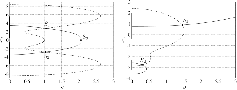
Figure 2: Singularities of the Ernst potential: The plots show, for two different configurations, curves along which the real part (solid curve) and imaginary part (dashed curve) of the determinant in the denominator of the Ernst potential $f$ vanish. At the intersection points $S_{1}$, $S_{2}$, ($S_{3}$), the Ernst potential diverges. The horizons $\mathcal{H}_{1}$, $\mathcal{H}_{2}$ are marked as black lines on the $\zeta$-axis.
Parameters: $\phi=\frac{3}{4}\pi$, $w=10/3$, $w^{\prime}=0.3$ (left panel) and $\phi=-0.1$, $w=1.3$, $w^{\prime}=0.5$ (right panel).

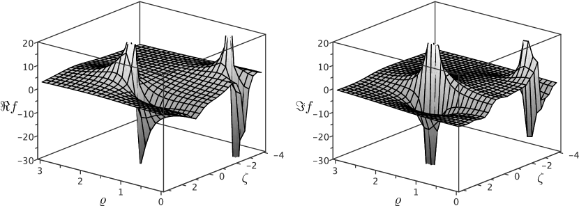
Figure 3: Singular Ernst-Potential: Real and imaginary part of the Ernst potential $f$ for the example configuration in Fig. 2, right panel.

6 Summary

The stationary equilibrium of two aligned rotating black holes can be described by a boundary value problem for two separate (Killing-) horizons (see Fig. 1). Applying the inverse (scattering) method, one can show that the solution of the problem is a (particular case of the) double-Kerr-NUT solution (a solution originally generated by a two-fold Bäcklund transformation of Minkowski space). The regularity conditions to be satisfied by the metric on the axis of symmetry outside the two horizons restrict the number of free parameters entering the solution. The resulting 3-parameter solution (written in dimensionless coordinates) does not satisfy the characteristic condition $8\pi|J|<A$ for each of the two black holes ($J$: angular momentum, $A$: area of the horizon). Since this inequality is a consequence of the geometry of trapped surfaces in the interior vicinity of the event horizon of every sub-extremal black hole, there exists no stationary equilibrium configuration for two aligned sub-extremal black holes.

- (1) Ansorg, M. and Petroff, D.: Negative Komar mass of single objects in regular, asymptotically flat spacetimes. Class. Quantum Grav. 23, L81 (2006)
- (2) Ansorg, M. and Hennig, J.: The inner Cauchy horizon of axisymmetric and stationary black holes with surrounding matter. Class. Quantum Grav. 25, 222001 (2008)
- (3) Ansorg, M. and Hennig, J.: The inner Cauchy horizon of axisymmetric and stationary black holes with surrounding matter in Einstein-Maxwell theory. Phys. Rev. Lett. 102, 221102 (2009)
- (4) Bardeen, J. M., Carter, B., and Hawking, S. W.: The four laws of black hole mechanics. Commun. Math. Phys. 31, 161 (1973)
- (5) Beig, R. and Schoen, R. M.: On static -body configurations in relativity. Class. Quantum Grav. 26, 075014 (2009)
- (6) Booth, I. and Fairhurst, S.: Extremality conditions for isolated and dynamical horizons. Phys. Rev. D 77, 084005 (2008)
- (7) Carter, B.: Black hole equilibrium states in Black Holes (Les Houches), edited by C. deWitt and B. deWitt, Gordon and Breach, London (1973)
- (8) Dietz, W. and Hoenselaers, C.: Two mass solution of Einstein’s vacuum equations: The double Kerr solution. Ann. Phys. 165, 319 (1985)
- (9) Hennig, J., Ansorg, M., and Cederbaum, C.: A universal inequality between the angular momentum and horizon area for axisymmetric and stationary black holes with surrounding matter. Class. Quantum Grav. 25, 162002 (2008)
- (10) Hennig, J., Cederbaum, C., and Ansorg, M.: A universal inequality for axisymmetric and stationary black holes with surrounding matter in the Einstein-Maxwell theory. arXiv:0812.2811 (2008)
- (11) Hennig, J. and Ansorg, M.: The inner Cauchy horizon of axisymmetric and stationary black holes with surrounding matter in Einstein-Maxwell theory: study in terms of soliton methods. arXiv:0904.2071 (2009)
- (12) Hoenselaers, C. and Dietz, W.: Talk given at the GR10 meeting, Padova (1983)
- (13) Hoenselaers, C.: Remarks on the Double-Kerr-Solution. Prog. Theor. Phys. 72, 761 (1984)
- (14) Kihara, M. and Tomimatsu, A.: Some properties of the symmetry axis in a superposition of two Kerr solutions. Prog. Theor. Phys. 67, 349 (1982)
- (15) Kramer, D. and Neugebauer, G.: The superposition of two Kerr solutions. Phys. Lett. A 75, 259 (1980)
- (16) Kramer, D.: Two Kerr-NUT constituents in equilibrium. Gen. Relativ. Gravit. 18, 497 (1986)
- (17) Krenzer, G.: Schwarze Löcher als Randwertprobleme der axislsymmetrisch-stationären Einstein-Gleichungen. PhD Thesis, University of Jena (2000)
- (18) Manko, V. S., Ruiz, E., and Sanabria-Gómez, J. D.: Extended multi-soliton solutions of the Einstein field equations: II. Two comments on the existence of equilibrium states. Class. Quantum Grav. 17, 3881 (2000)
- (19) Manko, V. S. and Ruiz, E.: Exact solution of the double-Kerr equilibrium problem. Class. Quantum Grav. 18, L11 (2001)
- (20) Neugebauer, G.: Bäcklund transformations of axially symmetric stationary gravitational fields. J. Phys. A 12, L67 (1979)
- (21) Neugebauer, G.: A general integral of the axially symmetric stationary Einstein equations. J. Phys. A 13, L19 (1980)
- (22) Neugebauer, G.: Recursive calculation of axially symmetric stationary Einstein fields. J. Phys. A 13, 1737 (1980)
- (23) Neugebauer, G.: Rotating bodies as boundary value problems. Ann. Phys. (Leipzig) 9, 342 (2000)
- (24) Neugebauer, G. and Meinel, R.: Progress in relativistic gravitational theory using the inverse scattering method. J. Math. Phys. 44, 3407 (2003)
- (25) Smarr, L.: Mass formula for Kerr black holes. Phys. Rev. Lett. 30, 71 (1973); Erratum: Phys. Rev. Lett. 30, 521 (1973)
- (26) Tomimatsu, A. and Kihara, M.: Conditions for regularity on the symmetry axis in a superposition of two Kerr-NUT solutions. Prog. Theor. Phys. 67, 1406 (1982)
- (27) Weyl, H.: Das statische Zweikörperproblem in Neue Lösungen der Einsteinschen Gravitationsgleichungen. Mathemat. Z. 13, 142 (1922)
- (28) Yamazaki, M.: Stationary line of Kerr masses kept apart by gravitational spin-spin interaction. Phys. Rev. Lett. 50, 1027 (1983)