Manifestly gauge invariant discretizations of the Schrödinger equation

Abstract

Grid-based discretizations of the time dependent Schrödinger equation coupled to an external magnetic field are converted to manifest gauge invariant discretizations. This is done using generalizations of ideas used in classical lattice gauge theory, and the process defined is applicable to a large class of discretized differential operators. In particular, popular discretizations such as pseudospectral discretizations using the fast Fourier transform can be transformed to gauge invariant schemes. Also generic gauge invariant versions of generic time integration methods are considered, enabling completely gauge invariant calculations of the time dependent Schrödinger equation. Numerical examples illuminating the differences between a gauge invariant discretization and conventional discretization procedures are also presented.

I Introduction

The fundamental laws of physics can (without exceptions) be related to certain continuous symmetries. In other words, by requiring that a model should be invariant with respect to a certain symmetry, the model is more or less completely determined. The Standard model of particle physics Peskin and Schroeder (1995); Weinberg (2002); Quigg (1997) and Gravitation Misner et al. (1973) are examples of such theories.

As an example, a model with a complex scalar field, i.e., a model of charged bosons, and a requirement of local $U(1)$-invariance, or gauge invariance, will immediately yield the Maxwell-Klein-Gordon (MKG) theory, which in the non-relativistic limit reduces to Maxwell-Schrödinger theory. In addition to defining the theory, the continuous symmetries give rise to conserved quantities through Noether’s theorem(s) Olver (2000); Goldstein et al. (2002); Rubakov (2002), and the local $U(1)$-symmetry of the MKG-model ensures the conservation of local electric charge.

In particle physics, and especially in the QCD-part of the standard model, numerical calculations are often done using Lattice Gauge Theory (LGT) Wilson (1974); Rothe (2005); Creutz (1986). This is a numerical procedure, actually motivated from the continuous theory, designed to preserve the underlying continuous gauge symmetry. In a previous article this discretization scheme was applied to the MKG-equation, with emphasis on the continuous $U(1)$-symmetry and conservation laws deduced from discrete versions of Noether’s theorem(s) Christiansen and Halvorsen (2008). By preserving the $U(1)$-symmetry of the MKG-model on the discrete level, a discrete equivalent of the conservation of local electric charge is immediate, which not only makes the scheme consistent, but is also a good indicator of stability. By a more standard discretization of the model, the local $U(1)$-symmetry is broken, which again implies that the scheme is not consistent with the continuous formulation. This will also reveal itself through the fact that the physical observables calculated are dependent on the gauge chosen, obviously in conflict with the continuous model.

A similar breaking of the continuous local $U(1)$-symmetry has been a known issue with discretizations of the Schrödinger equation coupled to an external electromagnetic field. For example in atomic physics, results are known to depend on the gauge in which the calculation is done Madsen (2002) – a most unfortunate situation indicating that the calculations are not correct. Gauge dependence also leads to interpretation problems of the results. It is the goal of the present paper to show how gauge invariant discretizations may be built from existing ones with little or no extra effort in the implementations.

Simple gauge invariant grid discretizations of Schrödinger operators have been studied in previous articles in the LGT formalism with promising results Governale and Ungarelli (1998); Andlauer et al. (2008); Janecek and Krotscheck (2008). The key to success in LGT is that it does not approximate the covariant derivative as a linear combination of the gradient and the gauge potential, an element of the Lie-algebra under consideration, since such an approximation leads to non-local terms when discretizing the gradient, and a question of gauge invariance is meaningless since one compare fields at different spacetime points. Instead LGT uses Forward-Euler/central difference approximation of the gradient in the various directions, which as argued is not gauge invariant, and then defines the covariant derivative through the way non-local terms are made gauge invariant in the continuous theory. This is done via the Wilson line Wilson (1974); Peskin and Schroeder (1995), to be discussed in the next section, which effectively localize non-local terms by parallel transport with the gauge potential as a key ingredient. By defining the covariant derivative in this way, the discrete theory is immediately manifestly gauge invariant.

The aim of this article is to expand the LGT formulation to allow for completely general grid discretizations in arbitrary local coordinates of the spatial manifold. Grid discretizations are widely used, and include most numerical discretizations of Schrödinger operators in use today, such as pseudospectral methods based on the discrete Fourier transform or Chebyshev polynomials. We also generalize the discussion to arbitrary coordinate systems, and some care is needed in case some of the coordinates are periodic when using global approximations (e.g., Chebyshev or Fourier expansions).

The paper is organized as follows: In Section II we introduce the time dependent Schrödinger equation in general coordinates. In Section III and IV we discuss gauge invariant spatial grid discretizations. We proceed in Section V to discuss gauge invariant time integration. Finally, in Section VI we present some numerical results shedding light on the difference between gauge invariant and gauge dependent schemes, before we close with some concluding remarks in Section VII.

II The time dependent Schrödinger equation and gauge invariance

We consider a particle with charge $q$ and mass $m$ coupled to an external electromagnetic (EM) field Shankar (1994) $(\mathbf{E},\mathbf{B})$. This is a semiclassical approach because the EM-field is obviously affected by the particle, but if we assume that the coupling is weak the approximation can be justified. We will work in the non-relativistic regime, but our considerations could easily be transmitted to a relativistic model. Moreover, the generalization to more than one particle is straightforward, since the EM fields only enter a many-body Hamiltonian at the one-body level, i.e., the interparticle interactions are independent of the EM fields.

We are considering a spacetime domain $\mathbb{R}\times\mathcal{M}$, with coordinates $(t,y)$, where $t\in\mathbb{R}$ is the time coordinate, and $y\in\mathcal{M}$ is a point in the spatial domain, usually taken to be Euclidean space, but can in general be a Riemannian manifold. In any case, we may work in local coordinates $x=(x^{i})$, viz, $y=y(x)\in\mathcal{M}$, with the induced metric tensor $g_{ij}(x)$ assumed to be time-independent. The wavefunction at some time $t$ is then a complex valued scalar function $x\mapsto\psi(x)$. In addition, the EM-field is described by a gauge potential $(t,x)\mapsto\phi(t,x)dt+A(t,x)$, where $\phi$ is a real valued function and $A$ is a real valued one-form. In coordinate basis one usually identifies one-forms with vectors. Thus, if $\{dx^{i}\}$ are basis one-forms and $\{\mathbf{e}_{i}\}$ are basis vectors there is a one-to-one correspondence between $A=A_{i}dx^{i}$ and $\mathbf{A}=A^{i}\mathbf{e}_{i}$. Note, we use the Einstein summation convention except where noted. The components of $A$ and $\mathbf{A}$ are related by the metric, i.e. $A^{i}=g^{ij}A_{j}$, and the physical EM fields $(\mathbf{E},\mathbf{B})$ are given by

$$\mathbf{E}=-\nabla\phi-\partial_{t}\mathbf{A},\qquad\mathbf{B}=\operatorname{curl}\mathbf{A},$$ (1)

where we use the shorthand $\partial_{t}=\partial/\partial t$.

In the following we work in units such that $\hbar=1$. The dynamics of the system is governed by the time dependent Schrödinger equation reading

$$\mathrm{i}D_{t}\psi(t,x)=\left[-\frac{1}{2m}\Delta_{A}+V(t,x)\right]\psi(t,x),$$ (2)

where $D_{t}=\partial_{t}+\mathrm{i}q\phi$ is the covariant derivative in the temporal direction, and where the “covariant Laplace-Beltrami” operator $\Delta_{A}$ is defined by

$$\Delta_{A}\equiv\frac{1}{\sqrt{g(x)}}D_{j}\sqrt{g(x)}g^{jk}D_{k},$$ (3)

with $D_{k}=\partial_{k}-\mathrm{i}qA_{k}$ being the covariant derivative in the direction $k$. Moreover, $p_{k}=-\mathrm{i}D_{k}$ is the (generalized) canonical momentum operator. The term $-\Delta_{A}/2m$ is simply the kinetic energy operator, and $V(t,x)$ is an external potential.

A fundamental property of the time dependent Schrödinger equation is that it is invariant under local gauge transformations, i.e. equation (2) is invariant under the following set of transformations

$$\psi(t,x) \mapsto e^{\mathrm{i}q\lambda(t,x)}\psi(t,x),$$ (4)

$$\phi(t,x) \mapsto \phi(t,x)-\partial_{t}\lambda(t,x),$$ (5)

$$A(t,x) \mapsto A(t,x)+\nabla\lambda(t,x),$$ (6)

where $(t,x)\mapsto\lambda(t,x)$ is a real valued function meaning that $\mathrm{i}q\lambda(t,x)\in\mathfrak{u(1)}$, the Lie-algebra of $U(1)$ (consult e.g. Olver (2000); Helgason (1978) for theory on Lie-groups and Lie-algebras). One says that the theory is invariant under local $U(1)$-transformations, meaning that the physical observables are not affected by the transformations. In particular, we note that the electric and magnetic fields (1) are not affected by the transformations (6). Moreover, if $X_{A}=X_{A}[(p^{j}),(x^{j})]$ is an observable, then the expectation value $\langle\psi,X_{A}\psi\rangle$ is gauge invariant, viz,

$$\langle e^{\mathrm{i}q\lambda}\psi,X_{A+\nabla\lambda}e^{\mathrm{i}q\lambda}\psi\rangle=\langle\psi,X_{A}\psi\rangle,$$ (7)

where $\langle\cdot,\cdot\rangle$ denotes the standard inner product in $L^{2}(\mathcal{M})$.

The usual way to write Eqn. (2) is

$$\mathrm{i}\partial_{t}\psi(t,x) = H(t)\psi(t,x)$$

$$:= \left[-\frac{1}{2m}\Delta_{A}+V(t,x)+q\phi(t,x)\right]\psi(t,x),$$

where the Hamiltonian $H(t)$ depends on the fields $(A,\phi)$. It is well-known that for any two $t$,$t^{\prime}$, the formal solution to (II) is given by $\psi(t,x)=\mathcal{U}(t,t^{\prime})\psi(t,x^{\prime})$, where the propagator $\mathcal{U}$ is

$$\mathcal{U}(t,t^{\prime})=\mathcal{T}\exp\left(-\mathrm{i}\int_{t^{\prime}}^{t}H(s)\,ds\right),$$ (9)

with $\mathcal{T}$ being the standard time-ordering operator. The propagator depends on the fields $(A,\phi)$ in the case of the current Hamiltonian, and under a gauge transformation with parameter $\lambda(t,x)$ we have

$$\mathcal{U}_{A^{\prime},\phi^{\prime}}(t,t^{\prime})=e^{\mathrm{i}q\lambda(t)}\mathcal{U}_{A,\phi}(t,t^{\prime})e^{-\mathrm{i}q\lambda(t^{\prime})},$$ (10)

where $A^{\prime}=A+\nabla\lambda$ and $\phi^{\prime}=\phi-\partial_{t}\lambda$.

III Discretization on a spatial grid

Many discretizations of Eqn. (2) approximate the wave function $\psi(t,x)$ at a given time $t\in\mathbb{R}$ on a finite grid $G$ (i.e., $y(G)\subset\mathcal{M}$) in order to obtain a semi-discrete formulation in which $\psi(t,\cdot)\in L^{2}[y(G)]$ still depends continuously on time. We shall here consider grids which in the local coordinates are Cartesian products of one-dimensional grids, i.e.,

$$G=G^{1}\times G^{2}\times\cdots\times G^{n},$$ (11)

where

$$G^{j}=\{x^{j}_{1},x^{j}_{2},\cdots,x^{j}_{N_{j}}\},\quad x^{j}_{k}<x^{j}_{k+1}.$$ (12)

Figure 1 illustrates this in the case of polar coordinates in the plane.

We may list the elements of $G$ using multi-indices, i.e.,

$$G=\left\{x_{\alpha}=(x^{1}_{\alpha_{1}},\cdots,x^{n}_{\alpha_{n}})\;:\;\forall j,\;0\leq\alpha_{j}<N_{j}\right\},$$ (13)

and the multi-indices may again be mapped one-to-one with $\{0,1,\cdots,N-1\}$, where $N=N_{1}N_{2}\cdots N_{n}$ is the total number of grid points. Thus, we obtain a discrete Hilbert space $\mathcal{H}(G)\simeq L^{2}[y(G)]$ of dimension $N$.

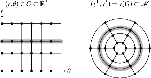
Figure 1: A grid in polar coordinates. In local coordinates $(r,\theta)\in\mathbb{R}^{2}$ the grid $G$ is a Cartesian product, while in on the manifold $\mathcal{M}\subset\mathbb{R}^{2}$ the grid instead has a (discrete) rotational symmetry. A coordinate curve for constant $r$ is also illustrated. In this case, the curve becomes a circle.

The natural basis to use in the space $\mathcal{H}(G)$ is the set of functions $e_{\alpha}$ such that $e_{\alpha}(x_{\beta})=\delta_{\alpha\beta}$. These functions are referred to as the cardinal basis Boyd (2001) or the nodal basis. For any $\psi\in\mathcal{H}(G)$, we now have

$$\psi=\sum_{\alpha}\psi(x_{\alpha})e_{\alpha}.$$ (14)

A linear operator $X$ on $\mathcal{H}$ may be represented by its action on this basis, which determines an $N\times N$ matrix with elements $X_{\alpha\beta}$, viz,

$$X_{\alpha\beta}\equiv[Xe_{\alpha}](x_{\beta}).$$ (15)

Thus, for $\psi\in\mathcal{H}(G)$,

$$[X\psi](x_{\alpha})=\sum_{\beta}X_{\alpha\beta}\psi(x_{\beta}).$$ (16)

At times, we will omit the brackets and write $X\psi(x_{\alpha})$ for the product $X\psi$ evaluated at $x_{\alpha}$, as usually there is no danger of confusion. Likewise, multiplication by $u\in\mathcal{H}(G)$ (or any continuous $u$ over $\mathcal{M}$) defines a linear operator, and for $\psi\in\mathcal{H}(G)$ we will write this simply as $u\psi$.

The grid discretization invariably comes with a discrete approximation to the (field-free, i.e., $A=0$) Laplace-Beltrami operator $\Delta_{0}$, although the exact procedure to fix this discrete operator may vary. We may assume that this discretization is composed of discrete derivatives in each spatial direction $x^{j}$ composed with some fixed functions of the coordinates, but the exact form is of no consequence to us.

To clarify these statements, consider for example Cartesian coordinates in two spatial dimensions for which $\Delta_{0}=\partial_{x}^{2}+\partial_{y}^{2}$. In a finite difference approximation we typically have a standard 5-point central difference stencil, i.e.,

$$\Delta_{0}\psi(x^{1},x^{2})\approx-(\delta_{1}^{\dagger}\delta_{1}+\delta_{2}^{\dagger}\delta_{2})\psi(x^{1},x^{2}),$$ (17)

where $\delta_{j}$ is a forward difference, $-\delta_{j}^{\dagger}$ a backward difference, so that $-\delta_{j}^{\dagger}\delta_{j}$ is the standard 3-point central difference operator in the $x^{j}$-direction, viz,

$$-\delta_{j}^{\dagger}\delta_{j}f(x^{j})\equiv\frac{1}{h^{2}}[f(x^{j}+h)-2f(x^{j})+f(x^{j}-h)],$$ (18)

with $h$ being the mesh width. We have suppressed other spatial coordinates than $x_{j}$ in the latter equation.

As a different example, consider polar coordinates $(x^{1},x^{2})=(r,\theta)$ in two dimensions, for which

$$\Delta_{0}=\frac{1}{r}\partial_{r}r\partial_{r}+\frac{1}{r^{2}}\partial_{\theta}^{2}.$$ (19)

The form of the radial part of this operator leads initially to several different schemes by either expressing it as

$$\frac{1}{r}\partial_{r}r\partial_{r}=\partial_{r}^{2}+\frac{1}{r}\partial_{r}$$ (20)

and then discretizing, or instead attack the original difference operator. In a general coordinate system there will of course be even more possibilities.

In any case, the discrete Laplace-Beltrami operator will be on the form

$$\Delta_{0}\approx\Delta_{0,h}=\Delta_{0,h}(\delta_{j},\delta_{j}^{2},x),$$ (21)

where $\delta^{k}_{j}$ are arbitrary approximations to each partial derivative $\partial^{k}_{j}$. We abuse notation a little, as in general we allow $\delta^{k}_{j}\neq(\delta^{1}_{j})^{k}$. In the Cartesian coordinate example above, $\delta^{2}_{j}=-\delta_{j}^{\dagger}\delta_{j}$. In general, however, we assume that like in this example, $\delta_{j}^{k}$ is the product of $k$ discrete derivative operators $\delta_{j,\ell}$, $1\leq\ell\leq k$, so that

$$\Delta_{0}\approx\Delta_{0,h}=\Delta_{0,h}(\delta_{j,k},x),$$ (22)

with $\delta_{j,0}=\delta_{j}$.

The usual way to discretize $\Delta_{A}$, on the other hand, which we here will call a “naïve” discretization, is to employ a similar “recipe” as in the examples to Eqn. (3) after insertion of $D_{j}=\partial_{j}-iqA_{j}$ and simplifying the expression. This, however, always leads to non-gauge invariant discretizations, as we will discuss in Section IV.

As an example of the naïve approach, consider again the polar coordinate case, and for simplicity assume $A_{r}=0$ for which we obtain

$$\Delta_{A} = \frac{1}{r}\partial_{r}r\partial_{r}+\frac{1}{r^{2}}(\partial_{\theta}-\mathrm{i}qA_{\theta})^{2}$$

$$= \Delta_{0}-\mathrm{i}q\frac{1}{r^{2}}(\partial_{\theta}A_{\theta}+A_{\theta}\partial_{\theta})-\frac{q^{2}}{r^{2}}A_{\theta}^{2}.$$

Assuming further that $\partial_{\theta}A_{\theta}=0$, i.e., that $A$ is given in the Coulomb gauge, we get

$$\Delta_{A}=\Delta_{0}-\mathrm{i}2q\frac{1}{r^{2}}A_{\theta}\partial_{\theta}-\frac{q^{2}}{r^{2}}A_{\theta}^{2}.$$ (23)

The naïve discretization of Eqn. (23) is then given by inserting the usual grid discretizations of $\partial_{r}$, $\partial_{r}^{2}$ and $\partial_{\theta}^{2}$.

Our prescription for a manifestly gauge invariant discretization of $\Delta_{A}$ in Eqn. (3) is simply to replace all occurrences of approximations $\delta_{j,k}$ of $\partial_{j}$ in the field-free naïve discretization with a certain corresponding approximation $\tilde{D}_{j,k}$ to $D_{j}$, derived using methods from LGT as mentioned in the Introduction, and whose final expression is given in Eqn. (49) below. In other words,

$$\Delta_{A}\approx\Delta_{0,h}(\tilde{D}_{j,k},x),$$ (24)

which will be gauge invariant. This approximation is often quite different from the standard naïve discretization.

IV Definition of the discrete covariant derivative

IV.1 One dimensional manifolds

IV.1.1 Gauge transformations

Consider first the case when $\mathcal{M}$ is a one-dimensional manifold $\mathcal{M}=\mathcal{M}^{1}\subset\mathbb{R}^{n}$. The reason for this is that in the general case, the differentiation operator $\partial_{j}$ can be viewed as a differential operator on the coordinate curves, these being one-dimensional manifolds. Similarly, a generic discrete $\delta_{j}$ can be viewed as an operator acting on grid functions over the one-dimensional “coordinate grids” obtained by fixing all but the $j$’th component of the multi-index $\alpha$ in Eqn. (13). Equivalently, $\delta_{j}$ defines a discrete differentiation operator acting on functions over a discretization of the coordinate curve; see Fig. 1.

Any one-dimensional manifold $\mathcal{M}$ will either be topologically equivalent to a circle or an interval, which may be bounded or unbounded. For example, in polar coordinates $(x^{1},x^{2})=(r,\theta)$ in $\mathbb{R}^{2}$ the angular coordinate curves are circles of radius $r$ while the radial coordinate curves are rays from the origin $r=0$ to infinity with an angle $\theta$ relative to the $x$-axis.

We write $x=x^{1}$ for the sole coordinate, omit the time dependence, and $D_{A}=\partial_{x}-\mathrm{i}qA(x)$ for the covariant derivative. Under gauge transformations, $D_{A}$ transforms as

$$D_{A+\lambda^{\prime}}=\partial_{x}-\mathrm{i}q[A(x)+\lambda^{\prime}(x)]=e^{\mathrm{i}q\lambda(x)}D_{A}e^{-\mathrm{i}q\lambda(x)},$$ (25)

where $\lambda^{\prime}(x)=\partial_{x}\lambda(x)$. Intuitively, since $\mathcal{M}$ is one-dimensional, one should be able to transform away $A(x)$ completely, by selecting $\lambda^{\prime}=-A$. However, if $\mathcal{M}$ is (topologically) a circle (with the point $x=0$ identified with $x=L$, for simplicity), this is not possible: There are one-forms $A(x)$ which are not the derivative of some zero-form $\lambda(x)$. On the circle, it is precisely the constant functions $A(x)=A_{0}$, since then $\lambda(x)=A_{0}x+b$ is not a zero-form: it is not periodic in $x$ unless $A_{0}=0$! If, on the other hand, $\mathcal{M}$ is topologically an interval, $A(x)$ may be transformed away.

These considerations may become clearer when we observe that, locally, we may write

$$D_{A}=u(x)^{*}\partial_{x}u(x),$$ (26)

where

$$u(x)=\exp\left(-\mathrm{i}q\int^{x}A(s)\,ds\right).$$ (27)

Whenever $\mathcal{M}$ is topologically an interval, we can choose $\lambda^{\prime}=-A$, and this expression is global, since then

$$u(x)=\exp(\mathrm{i}q\lambda(x)).$$ (28)

For $\mathcal{M}$ being topologically a circle, no such $\lambda(x)$ exists globally, unless $A_{0}=0$.

IV.1.2 Local approximations

Let $\mathcal{H}(G)$ be the discrete Hilbert space corresponding to an $N$-point discretization of $\mathcal{M}=\mathcal{M}^{1}$, being either a circle or an interval as described above. Thus, $G\subset\mathcal{M}^{1}$ is given by

$$G=\{x_{1},x_{2},\cdots x_{N}\},\quad x_{k}<x_{k+1}.$$ (29)

In the case of a circle, we identify $x_{N+1}$ and $x_{1}$ to impose periodic boundary conditions. We let $h=\min(x_{k},x_{k+1})$ be the mesh width, and typically $h\sim 1/N$.

Let $\delta_{h}$ be a discrete differential operator on $\mathcal{H}(N)$, and we assume for the moment that $\delta_{h}$ is a local operator, in the sense that as $h\rightarrow 0$, only a finite number of points in the neighborhood of $x_{k}\in G$ are used to differentiate $\psi(x_{k})$. As a consequence, there is a largest $p>0$ such that for any smooth function $\psi(x)$ over $\mathcal{M}^{1}$,

$$\delta_{h}\psi(x_{k})=\partial_{x}\psi(x_{k})+O(h^{p}),$$ (30)

where the term $O(h^{p})$ is equal to the truncation error, and we say that $\delta_{h}$ is a $p$’th order approximation. Examples of local discretizations are finite differences of any order, but not pseudospectral methods using for example Chebyshev polynomials or the discrete Fourier transform.

For any (discrete or smooth) $\psi$, the naïve discretization $\hat{D}_{A,h}$ of $D_{A}$ reads

$$\hat{D}_{A,h}\psi(x_{k})=(\delta_{h}-\mathrm{i}qA)\psi(x_{k}).$$ (31)

This operator is not gauge invariant. Let $\lambda(x)$ be given, and consider

$$(\hat{D}_{A+\lambda^{\prime},h}e^{i\lambda}\psi)(x_{k}) = (\delta_{h}e^{\mathrm{i}q\lambda}\psi)(x_{k})-\mathrm{i}q(Ae^{\mathrm{i}q\lambda}\psi)(x_{k})$$

$$\neq e^{\mathrm{i}q\lambda}\hat{D}_{A,h}\psi(x_{k}).$$

Clearly, this comes about since

$$(\delta_{h}e^{\mathrm{i}q\lambda})(x_{k})=\mathrm{i}q\lambda^{\prime}(x_{k})\exp(\mathrm{i}q\lambda(x_{k}))+O(h^{p})$$

is only an approximation.

However, the continuous covariant derivative $D_{A}$ comes about if one tries to construct a gauge invariant classical field theory Peskin and Schroeder (1995): since for any differentiable $\psi$, $\psi(x)$ and $\psi(y)$ transforms differently if $x\neq y$, the limit

$$\lim_{h\rightarrow 0}\frac{1}{h}[\psi(x+h)-\psi(x)]$$ (32)

has no simple transformation law. Notice that for finite $h$, $[\psi(x+h)-\psi(x)]/h$ is the standard forward difference operator. We could just as well consider the limit

$$\lim_{h\rightarrow 0}\delta_{h}\psi(x)$$ (33)

for any local discrete differentiation operator.

Introducing a comparator function $U(x,y)$ with the transformation law

$$U(x,y)\longrightarrow e^{\mathrm{i}q\lambda(x)}U(x,y)e^{-\mathrm{i}q\lambda(y)},$$ (34)

we see that for any $y$, the function $U(x,y)\psi(y)$ transforms in the same way as $\psi(x)$. Explicitly, the comparator is given by

$$U(x,y)=e^{-\mathrm{i}q\int^{y}_{x}A(t)\,dt}.$$ (35)

For any finite $h$, consider again the discrete difference operator $\delta_{h}$ applied to $U(x,y)\psi(y)$, but acting on the variable $y$, i.e.,

$$\tilde{D}_{h}\psi(x_{k})\equiv[\delta_{h,y}U(x_{k},y)\psi(y)](x_{k}).$$ (36)

The notation implies that the discrete derivative is evaluated at $y=x_{k}$. This operator is obviously gauge invariant, so that

$$\tilde{D}_{A+\lambda^{\prime},h}(e^{i\lambda}\psi)(x_{k})=e^{i\lambda}\tilde{D}_{A,h}\psi(x_{k}).$$ (37)

The path from $x$ to $y$ is in general ambiguous if $\mathcal{M}$ is a circle: we may move either clockwise or anti-clockwise, and also through several revolutions before ending up at $y$. However, as $h\rightarrow 0$, we desire our discrete $\tilde{D}_{A,h}$ to converge to $D_{A}$. The truncation error does not vanish unless we choose the shortest path, with vanishing length. Then, Eqn. (30) implies that for any smooth $\psi(x)$,

$$[\tilde{D}_{A,h}\psi](x)=D_{A}\psi(x)+O(h^{p}).$$ (38)

IV.1.3 Global approximations

The fact that $\delta_{h}$ was a local approximation to the derivative was crucial above, as it allowed us to resolve path ambiguity. For a global approximation this is not the case.

A global approximation $d_{h}$ to $\partial_{x}$ in general has exponential order of approximation as it utilizes all grid points $x_{k}\in G$ to estimate the derivative. That is, for any smooth $\psi(x)$, the truncation error is $O(h^{N})=O(h^{1/h})$, i.e.

$$d_{h}\psi(x)=\partial_{x}\psi(x)+O(h^{N}),$$ (39)

so that the order of approximation in fact increases as $h\rightarrow 0$.

As $U(x,y)$ may depend on path, and as $x$ and $y$ have arbitrary separation in a global method, the limit $h\rightarrow 0$ does not resolve the path ambiguity.

The only way to overcome this, is to ensure that the comparator itself is path-independent. This is the case if and only if $A(x)=\partial_{x}\Lambda(x)$ for some smooth $\Lambda$, since then the fundamental theorem of analysis yields

$$\int_{x^{\prime}}^{x}A(t)\,dt=\Lambda(x)-\Lambda(x^{\prime}),$$ (40)

independently of the path taken. For $\mathcal{M}$ being a circle, this means that $A(x)$ must be the derivative of a periodic function.

We therefore decompose the one-form $A(x)$ as

$$A(x)=A_{0}+A_{1}(x),$$ (41)

where $A_{0}$ is a constant such that $A_{1}(x)=\partial_{x}\Lambda(x)$ for some smooth $\lambda(x)$. Formally, $A_{0}$ is the projection of $A(x)$ onto the orthogonal complement of the range $\partial_{x}$, i.e., $\operatorname{Ran}(\partial_{x})^{\bot}$. The decomposition (41) is unique and it always exists. We may say that $A_{1}$ is the “largest part of $A$ that may be transformed away.” We then obtain

$$D_{A}=e^{\mathrm{i}q\int^{x}A_{1}}(\partial_{x}-\mathrm{i}qA_{0})e^{-\mathrm{i}q\int^{x}A_{1}}$$ (42)

for the covariant derivative. It is clear that if $A_{0}$ is nonzero, it may never be transformed away using a gauge transformation.

In the case of $\mathcal{M}$ being an interval, $\operatorname{Ran}(\partial_{x})^{\bot}=\{0\}$ , implying $A_{0}=0$, and we get

$$D_{A}=e^{\mathrm{i}q\int^{x}A(t)\,dt}\partial_{x}e^{-\mathrm{i}q\int^{x}A(t)\,dt},$$ (43)

where any anti-derivative of $A(x)$ may be used. For $\mathcal{M}$ being a circle, however,

$$\operatorname{Ran}(\partial_{x})^{\bot}=\{\text{ constant functions }\},$$ (44)

since $\int A_{0}=A_{0}x+b$ is not periodic unless $A_{0}=0$. It is straightforward to show that

$$A_{0}=\langle A\rangle=\frac{1}{L}\int_{0}^{L}A(t)\,dt.$$ (45)

We define a modified path independent comparator given by

$$U(x,y)=\exp\left[-\mathrm{i}q\int^{y}_{x}(A(s)-A_{0})\;ds\right].$$ (46)

Since it is independent of path, we may write

$$U(x,y)=u^{*}(x)u(y),\quad u(x)\equiv U(x_{0},x),$$ (47)

where $x_{0}\in G$ is any reference point. Combining Eqns. (42) and (36) we get

$$\tilde{D}_{A,h}\psi(x_{k})\equiv[\delta_{h,y}U(x_{k},y)\psi(y)](x_{k})-\mathrm{i}qA_{0}\psi(x_{k}),$$ (48)

and using Eqn. (47) we may rewrite this as

$$\tilde{D}_{A,h}\psi(x_{k})\equiv u^{*}\delta_{h}u\psi(x_{k})-\mathrm{i}qA_{0}\psi(x_{k}),$$ (49)

which may be a more practical expression to implement. This covariant derivative is valid for any one-dimensional manifold topology and any discretization of the derivative, and we note that in particular for $A_{0}=0$, it is equivalent to the original expression (36) for local discrete derivatives.

IV.2 General manifolds

For global methods, the one-dimensional case necessitated the computation of $A_{0}$ given by Eqn. (45). As the covariant derivative in this case was gauge equivalent to using the naïve discretization with a constant $A(x)=A_{0}$, one may wonder what we have to gain from the approach in this case: Why not use the standard naïve discretization using this particular, and physically equivalent, gauge? Most manifolds are, however, not one-dimensional. In this section, the case of $\mathcal{M}=\mathcal{M}^{n}$ being a general $n$-dimensional manifold is treated by simply defining $\tilde{D}_{A,h}$ for each spatial direction. In this case it is in general not true that the method becomes gauge equivalent to a naïve discretization: we may not find an $A$ such that the problem may be solved with a naïve discretization. Said in another way, on $\mathcal{M}^{n}$, the splitting (41) becomes

$$A(x)=A_{0}(x)+\nabla\Lambda(x),$$ (50)

where $A_{0}\in\operatorname{Ran}(\nabla)^{\bot}$ is the part of $A$ which may not be transformed away, and this is of course not a constant function in general.

In the $i$’th direction, at the point $y(x)\in\mathcal{M}$, the continuous covariant derivative is given by

$$D(A)_{i}=\partial_{i}-\mathrm{i}qA_{i}(x),$$ (51)

being an operator that constructs the $i$’th component of a one-form field, i.e., $D(A)\psi(x)=[\nabla-\mathrm{i}qA(x)]\psi(x)$ is a one-form field with components $D(A)_{i}\psi(x)$.

As discussed in Section III, we are given discretized derivative operators $\delta_{i}$ (we suppress the subscript “$h$” in the sequel, and also the distinction between local and global discrete differentiation operators $d_{i}$) which only involves grid points along the $i$’th coordinate curve at $x_{\alpha}\in G=G^{1}\times G^{2}\times\cdots\times G^{n}$; see Fig. 1 for an illustration. Thus, $\delta_{i}$ may be viewed as a discrete derivative on discretization of a one-dimensional manifold (the $i$’th coordinate curve at $x_{\alpha}$) with grid $G^{i}$. From Section IV.1, we then have the discrete covariant derivatives $\tilde{D}(A)_{i}$ given by

$$\tilde{D}(A)_{i}\equiv u^{*}_{i}(x)\delta_{i}u_{i}(x)-\mathrm{i}qA_{0}(x)_{i},$$ (52)

where $A_{0}(x)_{i}$ is the quantity $A_{0}$ in Eqn. (41) for $D(A)_{i}$ – in general not a constant since it depends on the other coordinates $x^{j}$, $j\neq i$. Neither is it given by the decomposition (50). Moreover, $u_{i}(x)$ (or more precisely $u_{i}^{*}(x)u_{i}(y)$) is the corresponding path-independent comparator for differentiation in the $i$’th direction.

To be precise, we write out these quantities in the general case.

The quantity $A_{0}(x_{\alpha})_{i}$ is zero for coordinate curves that are topological intervals, such as the radial coordinate curves in polar coordinates. For periodic coordinates, such as the angle $\theta$ in polar coordinates, the coordinate curves are circles. In that case,

$$A_{0}(x_{\alpha})_{i}=\frac{1}{L_{i}(x_{\alpha})}\int_{0}^{L_{i}}A_{i}(x^{1},\cdots,x^{i-1},s,x^{i+1},\cdots)\;ds,$$ (53)

where $L_{i}$ is the length of the coordinate curve. In polar coordinates, $x_{\alpha}=(r_{\alpha},\theta_{\alpha})$, and $L_{i}=2\pi r_{\alpha}$.

The comparator function $u_{i}(x_{\alpha})$ is now given by

$$u_{i}(x_{\alpha})=\exp\left(-\mathrm{i}q\int_{0}^{x_{\alpha}^{i}}\left(A_{i}(\cdots,s,\cdots)-A_{0}(x_{\alpha})\right)\;ds\right),$$ (54)

where the arbitrary reference point has been chosen as $x_{\alpha}^{i}=0$.

Gauge invariance of $\tilde{D}(A)_{i}$ follows from the gauge invariance in the one-dimensional case. Clearly, gauge invariance necessitates calculating the comparator functions and $A_{0}(x)_{i}$. However, these enter the discretizations only as multiplicative operators which are diagonal in the nodal basis. It is therefore a one-time calculation inducing little overhead in general.

V Time discretization

Thus far we have studied a discretization of the time-dependent Schrödinger equation in continuous time. However, when solving the problem numerically one needs to discretize the model in time as well. Again, with inspiration from classical LGT this can be done manifestly gauge invariant for every scheme with a grid based approximation of the time derivative.

The standard way to propagate the Schrödinger equation (2) is to attack the form (II) instead, viz,

$$\mathrm{i}\partial_{t}\psi(t,x)=\left[-\frac{1}{2m}\Delta_{A}+V(t,x)+q\phi(t,x)\right]\psi(t,x),$$ (55)

and then use standard techniques to integrate, analogously to the naïve spatial discretizations. However, this will of course lead to non-gauge invariant solutions.

Let us consider how gauge invariant formulations of some simple schemes can be constructed. For simplicity, we will assume that the wave function $\psi(t,x)$ is only sampled at equally spaced points in time, i.e., $t_{n}=n\tau$ with $n=0,1,\ldots$. At each time $t_{n}$, we write $\psi^{n}\in\mathcal{H}(N)$ for the corresponding spatially discrete wave function.

Let $\delta_{t}=\partial_{t}+O(\tau^{k})$ be a local approximation, and assume that a naïve discretization of a generic Schrödinger equation with Hamiltonian $H(t)$ is given by

$$\mathrm{i}\delta_{t}\psi^{n}=\sum_{|j|\leq m}c_{j}H^{n+j}\psi^{n+j},$$ (56)

where $H^{n}$ is the Hamiltonian $H(t)$ evaluated at $t=n\tau$. Here, $c_{j}$ are constants, the notation indicating that only a finite number of such constants are involved. Such schemes include the standard implicit Crank-Nicholson and leap-frog schemes Askar and Cakmak (1978). For the Crank-Nicholson scheme, $\delta_{t}$ is the forward Euler discretization, while $c_{0}=c_{1}=1/2$ ($m=1$ and $c_{-1}=0$). For the Leap-Frog scheme, $\delta_{t}$ is the centered difference with step length $2\tau$ and $c_{0}=1$ (with $m=0$). Using similar considerations as in Section IV for spatial differentiation operators, the corresponding gauge invariant discretization of (2) for arbitrary fields $\phi$ becomes

$$\mathrm{i}\tilde{D}_{t}\psi^{n}=\sum_{|j|\leq m}\tilde{c}_{n,j}H_{A}^{n+j}\psi^{n+j},$$ (57)

where $\tilde{c}_{n,j}=c_{j}U(t_{n},t_{n+j})$, with

$$U(t,t^{\prime})=\exp\left(\mathrm{i}\int^{t^{\prime}}_{t}\phi(s)ds\right)$$ (58)

being the comparator for the time coordinate. The Hamiltonian $H_{A}(t)$ is given by

$$H_{A}(t)=-\frac{1}{2m}\Delta_{A}+V(t,x),$$ (59)

and excludes the term $q\phi(t,x)$ which is now absorbed into the covariant derivative $\tilde{D}_{t}$.

We now observe something peculiar: The scalar field $\phi(t,x)$ may be transformed away globally by the gauge parameter $\lambda=\int^{t}\phi(s)ds$, yielding the so-called temporal gauge. In this gauge $U(t,t^{\prime})=1$, so the gauge invariant scheme (57) reduces to the naïve scheme (56) – of course with a different Hamiltonian $H_{A+\nabla\lambda}$.

In fact, these considerations hold for any gauge invariant numerical integration scheme: gauge invariance implies that the temporal gauge in particular may be used, for which the integration method reduces to the naïve non-gauge invariant scheme applied to $H_{A+\nabla\lambda}$. Notice, however, that the latter operator is time dependent, even if $V$ and the fields $A$ and $\phi$ are time-independent functions.

To make this statement precise, let $\mathcal{U}_{h}(t+\tau,t)$ be a general numerical propagation scheme for a generic Hamiltonian $H(t)$, i.e., it approximates the propagator $\mathcal{U}(t+\tau,t)$ in Eqn. (9), viz,

$$\mathcal{U}(t+\tau,t)=\mathcal{U}_{h}(t+\tau,t)+O(\tau^{m}),$$ (60)

where $O(\tau^{m})$ is the truncation error of the scheme. Thus, the wave function $\psi^{n}$ is propagated by

$$\psi^{n+1}=\mathcal{U}_{h}(t+\tau,t)\psi^{n}.$$ (61)

Assuming that $\tilde{\mathcal{U}}_{A,\phi}$ is a gauge invariant generalization of $\mathcal{U}_{h}$ applied to the Hamiltonian $H_{A}$, it must transform according to Eqn. (10). The temporal gauge is achieved by selecting $\lambda=\Lambda$ given by

$$\Lambda(t,x)=\int^{t}_{0}\phi(x,s)\;ds,$$ (62)

which gives

$$A^{\prime}=A+\nabla\Lambda(t,x)=A+\nabla\int^{t}_{0}\phi(x,s)\;ds.$$ (63)

We obtain

$$\tilde{\mathcal{U}}_{A,\phi}(t,t^{\prime})=e^{\mathrm{i}q\Lambda(t)}\tilde{\mathcal{U}}_{A+\nabla\Lambda,0}(t,t^{\prime})e^{-\mathrm{i}q\Lambda(t^{\prime})},$$ (64)

where $\tilde{\mathcal{U}}_{A+\nabla\Lambda,0}$ must be equal to the original gauge dependent propagator applied to the Hamiltonian $H_{A+\nabla\Lambda}$.

It is not always easy to identify an expression for $\tilde{\mathcal{U}}_{A,\phi}(t,t^{\prime})$ in a general gauge, but from the above considerations, the temporal gauge is sufficient anyway.

The selection of a particular gauge for time integration may seem unnatural. However, it is the structure of the Schrödinger equation together with the fact that any field $\phi$ may be transformed away that yields this conclusion. The vector potential $A$ cannot in general be transformed away – therefore we should not choose a particular gauge for spatial operators.

VI Numerical example

In Ref. Governale and Ungarelli (1998), some promising gauge invariant eigenvalue calculations are shown using the classical LGT formalism, i.e., with standard finite differences in space. In Ref. Janecek and Krotscheck (2008) higher-order finite differences are used, and the results are equally promising. Even though the published experiments are all with the “standard” example of a uniform magnetic field in the $z$-direction applied to a planar system, there is little doubt that the gauge invariant formulations offer favorable properties over the non-gauge invariant methods, as there are always gauges that behave very badly. One may simply choose a rapidly oscillating gauge parameter $\lambda(t,x)$ to completely destroy the accuracy. Choosing the “right gauge” in a non-gauge invariant scheme may not at all be simple or even possible. In any case, a gauge independent method will “factor out” any non-physical effect of the choice of gauge, making interpretations easier, and it is reasonable to expect that gauge invariance should stabilize the discretization because of this.

We focus here on time integration only. The benefit of employing spatially gauge invariant schemes has already been established in e.g. Governale and Ungarelli (1998). A gauge invariant discretization of the time-dependent Schrödinger equation could enable practitioners to push the limits of what is possible to compute and interpret.

We consider a single particle in a one-dimensional system; a very simple system but one whose numerical properties are reflected in more realistic settings. We set $m=q=1$, and consider the Schrödinger equation (2) on the form

$$\mathrm{i}[\partial_{t}+\mathrm{i}\phi(t,x)]\psi(t,x)=-\frac{1}{2}[\partial_{x}-iA(t,x)]^{2}\psi(t,x).$$ (65)

We consider a spatial truncation $[-L/2,+L/2]\subset\mathbb{R}$, and use a finite difference discretization with $N+2$ equally spaced grid points $x_{k}=kh\in G$, $k=0,1,\ldots,N+1$. The grid spacing is given by $h=L/(N+1)$. Thus, at a time $t$, $\psi(t,x)\approx\psi(t,x_{j})\in\mathcal{H}(G)$ is our discrete wave function.

A common situation in atomic physics arise when one considers the so-called dipole approximation Madsen (2002), in which the fields $A$ and $\phi$ take the form

$$\phi(t,x) = f(t)x$$

$$A(t,x) = 0,$$ (66)

corresponding to a time-dependent electric field $\mathbf{E}(t)=-f(t)\mathbf{e}_{x}$ and $\mathbf{B}=0$. These fields are of course not solutions of Maxwell’s equations. The particular gauge in Eqn. (66) is referred to as the length-gauge. The so-called velocity gauge is obtained by transforming away $\phi(t,x)$ using the gauge parameter $\lambda(t,x)=\int^{t}_{0}\phi(s,x)ds$, i.e., it is the temporal gauge. We obtain

$$\phi^{\prime}(t,x) = 0,$$

$$A^{\prime}(t,x) = \int^{t}_{0}\partial_{x}\phi(s,x)\,ds.$$ (67)

The wave functions in the two gauges are of course related by $\psi^{\prime}(t,x)=e^{i\lambda(t,x)}\psi(t,x)$. These two gauges are commonly studied, and may give different results in actual calculations; a sure sign of a significant error.

A common choice for $f(t)$ is

$$f(t)=c\sin(\omega t),$$ (68)

describing an oscillating electric field with frequency $\omega$.

Using finite differences, a typical naïve semi-discretization of Eqn. (65) is

$$\mathrm{i}\partial_{t}\psi(t,x_{j}) = \left[-\frac{1}{2}(\delta^{+}-\mathrm{i}A)(\delta^{-}-\mathrm{i}A)+\phi\right]\psi(t,x_{j})$$ (69)

$$= \frac{1}{2}\left[-\delta^{+}\delta^{-}+\mathrm{i}(A\delta^{-}+\delta^{+}A)+A^{2}+2\phi\right]\psi(t,x_{j}).$$

where $\delta^{+}$ is a forward difference, and $\delta^{-}$ is a backward difference. As earlier, $A$ and $\phi$ should be interpreted as diagonal multiplication operators. As $(\delta^{+})^{\dagger}=-\delta^{-}$, it is easy to see that the operator on the right hand side of Eqn. (69) is actually Hermitian.

The corresponding gauge invariant semi-discretization is, in the temporal gauge,

$$\mathrm{i}\partial_{t}\psi(t,x_{j})=\left[-\frac{1}{2}u^{*}\delta^{+}\delta^{-}u\right]\psi(t,x_{j}),$$ (70)

with $u(t,x)=\exp[-\mathrm{i}\lambda(t,x)+\mathrm{i}\lambda(t,0)]$ being the comparator function.

To integrate Eqns. (69) and (70) in time, we select a somewhat non-standard approach. It is well-known that an approximation to $\mathcal{U}(t+\tau,t)$ for a given Hamiltonian $H(t)$ is

$$\mathcal{U}(t+\tau,t)\approx\mathcal{U}_{\tau}(t)\equiv e^{-i\int_{t}^{t+\tau}H(s)ds},$$ (71)

where the error is $O(\tau^{2})$. Propagating $\psi^{n}\equiv\psi(t_{n},x_{j})\in\mathcal{H}(G)$ using $\mathcal{U}_{\tau}(t)$ gives an error increasing roughly linearly as function of the number of time steps. The integral is evaluated using Gauss-Legendre quadrature using two evaluation points, giving practically no error in the integral as long as $f(t)$ does not oscillate too rapidly.

We choose $c=5$ and $\omega=10$ for the electrical field, and integrate for $t_{n}=n\tau\leq 6\pi/\omega$, so that the electric field oscillate exactly three times before we terminate the calculation. The spatial domain is of length $L=40$, and we use $N=255$ points.

We choose $\psi(x,0)=\exp(-x^{2}/2)$ as initial condition (which is normalized numerically in the calculations). The analytic solution using this particular problem (on whole of $\mathbb{R}$) can be computed in closed form, but we choose instead to perform a reference calculation using a pseudospectral discretization using $N+1$ points and a much smaller time step, giving in this case practically no error.

Figure 2 shows the error $\|\psi^{n}-\psi_{\text{exact}}(t_{n})\|$ as function of $t$ in the three cases. Clearly, the velocity gauge has somewhat smaller error, and also the length gauge and gauge invariant calculations have almost indistinguishable errors. The latter fact can easily be understood by inserting $\psi^{\prime}=\exp(i\lambda)\psi$ into the semi-discrete formulations, and noting that $\delta^{+}\delta^{-}$ and $u^{*}\delta^{+}\delta^{-}u$ are unitarily equivalent, i.e., having the same eigenvalues. The semidiscrete equations are thus actually equivalent, and any discrepancy showing in the graphs for the gauge invariant scheme and the length-gauge calculation comes from errors in the time integration.

The spectrum of $(\delta^{+}-\mathrm{i}A)(\delta^{-}-\mathrm{i}A)$ is not equivalent to that of $\delta^{+}\delta^{-}$ when $A\neq 0$, however. In fact, it is readily established that the latter operator has eigenvalues depending strongly on $A$, and therefore on the particular gauge used. Hence, it is expected that the velocity gauge, or any other gauge in which $A\neq 0$, should perform worse than either of the other gauges in the generic case.

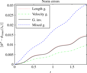
Figure 2: (Color online) Errors in the time-integration for the electric field $\mathbf{E}(t,x)=-c\sin(\omega t)\mathbf{e}_{x}$. The velocity gauge (dashed/dotted green) has somewhat larger error than the gauge invariant (solid black) and the length gauge (dotted red) calculations. The low error in the velocity gauge is a “stroke of luck” when compared with Fig. 3, where the velocity gauge has the largest error. Notice that the oscillations of the EM-fields clearly affect the errors.

To test this statement, we perform a calculation using a different field $\phi(t,x)$ in the length gauge, namely

$$\phi(t,x)=c\sin(\omega t-\mu x),$$ (72)

which may describe incoming electromagnetic waves (e.g., a laser) along the $x$ axis. Figure 3 shows the errors as function of $t$ in this case, using $\mu=1$, clearly showing that the velocity gauge indeed has the larger error. Moreover, a “mixed gauge” calculation is shown, where the length gauge fields are transformed using a gauge parameter $\lambda(t,x)=x$, chosen somewhat arbitrarily. Now, both $A$ and $\phi$ are non-vanishing, and the error is seen to behave accordingly.

We notice that the gauge invariant calculations in both cases are well-behaved, and no choice of gauge will of course affect the calculations. Moreover, the length gauge is equivalent to the gauge invariant calculations only when $A=0$; this holds in general in one dimensional systems, but of course not in arbitrary dimensions, where the magnetic field usually cannot be transformed away in this way.

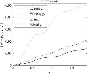
Figure 3: (Color online) Errors in the time-integration for the electric field $\mathbf{E}(t,x)=c\mu\cos(\omega t-\mu x)\mathbf{e}_{x}$. The gauge invariant (solid black) and the length gauge (dotted red) calculations have the smallest errors, while the velocity gauge (dot-dash, green) has clearly the largest error. This should be contrasted with the results in Fig. 2, where the velocity gauge has the smallest error.

VII Conclusion

We have discussed a method based on LGT to convert virtually any grid-based scheme for the time-dependent Schrödinger equation (II) to a gauge invariant scheme, in both space and time. We have considered discretization in arbitrary coordinates on arbitrary spatial manifolds. The theory is directly generalizable to many-particle systems as the EM-fields obviously only enter at one-body level in the many-body Hamiltonian. Moreover, the computational overhead of the gauge invariant schemes compared to the original ones are negligible.

Our numerical simulations of time-dependent problems, albeit simplistic, indicate that the gauge invariant schemes perform on average better than standard schemes, even though the original “naïve” scheme may be better in specific cases.

A further line of work would be to rigorously understand the accuracy gained by introducing gauge invariance.

References

- Peskin and Schroeder (1995) M. E. Peskin and D. V. Schroeder, An introduction to Quantum Field Theory (Westview Press, 1995), 1st ed.
- Weinberg (2002) S. Weinberg, The Quantum Theory of Fields, vol. 1 (Cambridge University Press, 2002).
- Quigg (1997) C. Quigg, Gauge Theories of the Strong, Weak, and Electromagnetic Interactions (Westview Press, 1997).
- Misner et al. (1973) C. W. Misner, Kip S. Thorne, and John Archibald Wheeler, Gravitation (W. H. Freeman and Company, New York, 1973).
- Olver (2000) P. J. Olver, Applications of Lie Groups to Differential Equations (Springer-Verlag, 2000), 2nd ed.
- Goldstein et al. (2002) Goldstein, Poole, and Safko, Classical Mechanics (Addison Wesley, 2002), 3rd ed.
- Rubakov (2002) V. Rubakov, Classical Theory of Gauge Fields (Princeton University Press, 2002), 1st ed.
- Wilson (1974) K. G. Wilson, Phys. Rev. D 10, 2445 (1974).
- Rothe (2005) H. J. Rothe, Lattice Gauge Theories, An Introduction (World Scientific, 2005), 3rd ed.
- Creutz (1986) M. Creutz, Quarks, gluons and lattices (Cambridge, 1986), 1st ed.
- Christiansen and Halvorsen (2008) S. H. Christiansen and T. G. Halvorsen, Tech. Rep., University of Oslo, Department of Mathematics, E-print No. 17,Pure Mathematics, ISSN 0806-2439 (2008).
- Madsen (2002) L. B. Madsen, Phys. Rev. A 65, 053417 (2002).
- Governale and Ungarelli (1998) M. Governale and C. Ungarelli, Phys. Rev. B 58, 7816 (1998).
- Andlauer et al. (2008) T. Andlauer, R. Morschl, and P. Vogl, Physical Review B 78 (2008), ISSN 1098-0121.
- Janecek and Krotscheck (2008) S. Janecek and E. Krotscheck, Physical Review B 77 (2008), ISSN 1098-0121.
- Shankar (1994) R. Shankar, Principles of Quantum Mechanics (Springer, 1994), ISBN 0306447908.
- Helgason (1978) S. Helgason, Differential Geometry, Lie Groups and Symmetric Spaces (Academic Press, 1978).
- Boyd (2001) J. Boyd, Chebyshev and Fourier Spectral Methods (Springer, 2001).
- Askar and Cakmak (1978) A. Askar and A. S. Cakmak, The Journal of Chemical Physics 68, 2794 (1978).