Cosmic Constraints on Holographic Dark Energy in Brans-Dicke Theory

Abstract

In this paper, the holographic dark energy in Brans-Dicke theory is confronted by cosmic observations from SN Ia, BAO and CMB shift parameter. The best fit parameters are found in $1\sigma$ region: $\Omega_{h0}=0.683^{+0.035}_{-0.038}$, $c=0.605^{+0.138}_{-0.107}$ and $\alpha=0.00662^{+0.00477}_{-0.00467}$ (equivalently $\omega=905.690^{+637.906}_{-651.471}$ which is less the solar system bound and consistent with other constraint results). With these best fit values of the parameters, it is found the universe is undergoing accelerated expansion, and the current value of equation of state of holographic dark energy $w_{h0}=-1.246^{+0.191}_{-0.144}$ which is phantom like in Brans-Dicke theory. The evolution of effective Newton’s constant is also explored.

TP-DUT/2009-05

I Introduction

The observation of the Supernovae of type Ia ref:Riess98 ; ref:Perlmuter99 provides the evidence that the universe is undergoing accelerated expansion. Jointing the observations from Cosmic Background Radiation ref:Spergel03 ; ref:Spergel06 and SDSS ref:Tegmark1 ; ref:Tegmark2 , one concludes that the universe at present is dominated by $70\%$ exotic component, dubbed dark energy, which has negative pressure and push the universe to accelerated expansion. Of course, the accelerated expansion can attribute to the cosmological constant naturally. However, it suffers the so-called fine tuning and cosmic coincidence problem. To avoid these problem, dynamic dark energy models are considered, such as quintessence ref:quintessence1 ; ref:quintessence2 ; ref:quintessence3 ; ref:quintessence4 , phtantom ref:phantom , quintom ref:quintom and holographic dark energy ref:holo1 ; ref:holo2 etc. For recent reviews, please see ref:DEReview1 ; ref:DEReview2 ; ref:DEReview3 ; ref:DEReview4 ; ref:DEReview5 ; ref:DEReview6 . In particular, the model, named holographic dark energy, is constructed by considering the holographic principle and some features of quantum gravity theory. According to the holographic principle, the number of degrees of freedom in a bounded system should be finite and has relations with the area of its boundary. By applying the principle to cosmology, one can obtain the upper bound of the entropy contained in the universe. For a system with size $L$ and UV cut-off $\Lambda$ without decaying into a black hole, it is required that the total energy in a region of size $L$ should not exceed the mass of a black hole of the same size, thus $L^{3}\rho_{\Lambda}\leq LM^{2}_{pl}$. The largest $L$ allowed is the one saturating this inequality, thus $\rho_{\Lambda}=3c^{2}M^{2}_{pl}L^{-2}$, where $c$ is a numerical constant and $M_{pl}$ is the reduced Planck Mass $M^{-2}_{pl}=8\pi G$. It just means a duality between UV cut-off and IR cut-off. The UV cut-off is related to the vacuum energy, and IR cut-off is related to the large scale of the universe, for example Hubble horizon, event horizon or particle horizon as discussed by ref:holo1 ; ref:holo2 . In the paper ref:holo2 , the author takes the future event horizon

$$R_{eh}(a)=a\int^{\infty}_{t}\frac{dt^{{}^{\prime}}}{a(t^{{}^{\prime}})}=a\int^{\infty}_{a}\frac{da^{{}^{\prime}}}{Ha^{{}^{\prime}2}}$$ (1)

as the IR cut-off $L$. This horizon is the boundary of the volume a fixed observer may eventually observe. One is to formulate a theory regarding a fixed observer within this horizon. As pointed out in ref:holo2 , it can reveal the dynamic nature of the vacuum energy and provide a solution to the fine tuning and cosmic coincidence problem. In this model, the value of parameter $c$ determines the property of holographic dark energy. When $c\geq 1$, $c=1$ and $c\leq 1$, the holographic dark energy behaviors like quintessence, cosmological constant and phantom respectively.

On the other hand, Brans-Dicke theory ref:BransDicke as a natural extension of Einstein’s general theory of relativity can pass the experimental tests from the solar system ref:solar and provide explanation to the accelerated expansion of the universe ref:BDEp1 ; ref:BDEp2 ; ref:BDEp3 . In Brans-Dicke theory, the gravitational constant is replaced with a inverse of time dependent scalar field, i.e. $8\pi G=\frac{1}{\Phi(t)}$, which couples to gravity with a coupling parameter $\omega$. The holographic dark energy model in the framework of Brans-Dicke theory which has already been considered by many authors ref:BDH1 ; ref:BDH2 ; ref:BDH3 ; ref:BDH4 ; ref:BDH5 ; ref:BransDicke . In our previous paper ref:BransDicke , the properties of holographic dark energy in Brans-Dicke theory was discussed by giving some characteristic values of the parameters, where the values of the parameters were given by taking the corresponding values obtained from constraint by cosmic observations in Einstein theory. However, in Brans-Dicke theory, the values of parameters would be different from that in Einstein theory. After all, the Newton’s constant $G$ evolves with time in Brans-Dicke theory. So, there would be some differences. In fact, in our previous paper ref:BransDicke , the value of $\left|\omega\right|>40000$ is taken for granted. It would be dangerous because of the possibility of small value in large scale, say in cosmological scale, reported by the authors ref:smallomega . So, the holographic dark energy in Brans-Dicke theory must be tested by cosmic observations. This is the main task of this work. In this paper, the cosmic observations from SN Ia, BAO and CMB shift parameter will be used as cosmic constraints, for details please see the following sections. When using these observational data set, one has to notice the evolution of Newton’s constant $G$. In fact, the SN Ia as a useful cosmic constraint has been considered in ref:smallomega ; ref:BDSN1 ; ref:BDSN2 ; ref:BDSN3 .

This paper is structured as follows. In Section II, we give a brief review of holographic dark energy in Brans-Dicke theory. A brief description of comic observations and methods used in our paper is listed in Section III. Section IV is the results and discussion.

II Holographic dark energy in Brans-Dicke theory

Here, we just give a brief review of holographic dark energy in Brans-Dicke theory, for the details please see ref:BDHD . The holographic dark energy in Brans-Dicke theory takes the form

$$\rho_{h}=3c^{2}\Phi(t)L^{-2},$$ (2)

where $\Phi(t)=\frac{1}{8\pi G_{eff}}$ is a reverse of time variable Newton’s constant. In a spatially flat FRW cosmology filled with dark matter and holographic dark energy, the gravitational equations can be written as

$$3\Phi\left[H^{2}+H\frac{\dot{\Phi}}{\Phi}-\frac{\omega}{6}\frac{\dot{\Phi}^{2}}{\Phi^{2}}\right]=\rho_{m}+\rho_{h},$$ (3)

$$2\frac{\ddot{a}}{a}+H^{2}+\frac{\omega}{2}\frac{\dot{\Phi}^{2}}{\Phi^{2}}+2H\frac{\dot{\Phi}}{\Phi}+\frac{\ddot{\Phi}}{\Phi}=-\frac{p_{h}}{\Phi},$$ (4)

where $H=\frac{\dot{a}}{a}$ is the Hubble parameter, $\rho_{m}$ is dark matter energy density, $\rho_{h}$ is the holographic dark energy density and $p_{h}$ is the pressure of holographic dark energy. The scalar field evolution equation is

$$\ddot{\Phi}+3H\dot{\Phi}=\frac{\rho_{m}+\rho_{h}-3p_{h}}{2\omega+3}.$$ (5)

Considering the dark matter energy conservation equation

$$\dot{\rho_{m}}+3H\rho_{m}=0,$$ (6)

and jointing it with Eq. (3), Eq. (4) and Eq. (5), one obtains the holographic dark energy conservation equation

$$\dot{\rho_{h}}+3H(\rho_{h}+p_{h})=0.$$ (7)

Here, we have considered non-interacting cases. The Friedmann equation (3) is

$$H^{2}=\frac{\rho_{m}+\rho_{h}}{3\Phi}-H\frac{\dot{\Phi}}{\Phi}+\frac{\omega}{6}\frac{\dot{\Phi}^{2}}{\Phi^{2}}.$$ (8)

With the assumption $\Phi/\Phi_{0}=(a/a_{0})^{\alpha}$, the Eq. (8) is rewritten as

$$H^{2}=\frac{2}{(6+6\alpha-\omega\alpha^{2})\Phi}(\rho_{m}+\rho_{h}).$$ (9)

It is easy to find out that, in the limit case $\alpha\rightarrow 0$, the standard cosmology is recovered. To make the Friedmann equation (9) to have physical meanings, i.e. to make $(6+6\alpha-\omega\alpha^{2})>0$, one has the following constraints on the values of $\alpha$

$$\begin{array}[]{ccc}\frac{3-\sqrt{9+6\omega}}{\omega}<\alpha<\frac{3+\sqrt{9+6\omega}}{\omega},&\text{for}&\omega>0,\\ \alpha<\frac{3-\sqrt{9+6\omega}}{\omega}\quad\text{or}\quad\alpha>\frac{3+\sqrt{9+6\omega}}{\omega},&\text{for}&-3/2\leq\omega<0,\\ \Re,&\text{for}&\omega<-3/2.\end{array}$$ (10)

However, the solar system experiments predict the value of $\omega$ is $\left|\omega\right|>40000$ ref:solar . However, the value of parameter $\omega=-3/2$ is a boundary of ghost ref:BDghost . So, in this paper, when considering these constraints, the second line of Eq. (10) will be omitted and $\omega>0$ will be consider in this paper. In fact, authors ref:BDCos have used the cosmic observations to constrain the parameter $\omega$. In ref:BDCos , the authors found that $\omega$ can be smaller than $40000$ in cosmological scale, say $\omega\sim 1000$.

When the event horizon $R_{eh}$

$$R_{eh}(a)=a\int^{\infty}_{t}\frac{dt^{{}^{\prime}}}{a(t^{{}^{\prime}})}=a\int^{\infty}_{a}\frac{da^{{}^{\prime}}}{Ha^{{}^{\prime}2}}$$ (11)

is taken as the IR cut-off. The holographic dark energy is

$$\rho_{h}=\frac{3c^{2}\Phi}{R^{2}_{eh}}.$$ (12)

And, the Friedmann Eq. (9) is rewritten as

$$H^{2} = H^{2}_{0}\Omega_{m0}\left(\frac{a_{0}}{a}\right)^{(3+\alpha)}+\Omega_{h}H^{2}$$ (13)

$$= H^{2}_{0}\Omega_{m0}a^{-(3+\alpha)}+\Omega_{h}H^{2},$$

where the dimensionless energy density of of dark matter is $\Omega_{m0}=\frac{2}{(6+6\alpha-\omega\alpha^{2})}\frac{\rho_{m0}}{\Phi_{0}H^{2}_{0}}\equiv\frac{8\pi G\rho_{m0}}{3H^{2}_{0}}$ and the one of holographic dark energy $\Omega_{h}$ is the solution of differential equation

$$\Omega_{h}^{\prime}=\Omega_{h}\left(1-\Omega_{h}\right)\left(1+\alpha+\frac{2}{c}\sqrt{\Omega_{h}}\right),$$ (14)

where ^′ denotes the derivative with respect to $x=\ln a$. This equation describes the evolution of dimensionless energy density of dark energy. Comparing the definition of $\Omega_{m0}$ with that of the standard cosmological model, one easily has the relation $\omega\alpha=6$. With the relation $a_{0}/a=1+z$, the Friedmann equation (13) can be rewritten as

$$H^{2}=H^{2}_{0}\frac{\Omega_{m0}a^{-(3+\alpha)}}{1-\Omega_{h}}=H^{2}_{0}\frac{\Omega_{m0}(1+z)^{(3+\alpha)}}{1-\Omega_{h}},$$ (15)

From the conservation equation of the holographic dark energy (7), on has the equation of state (EoS) of holographic dark energy

$$w_{h}=-1-\frac{1}{3}\frac{d\ln\rho_{h}}{d\ln a}=-\frac{1}{3}\left(1+\alpha+\frac{2}{c}\sqrt{\Omega_{h}}\right),$$ (16)

where $w_{h}=p_{h}/\rho_{h}$. From the above equation, one finds the EoS of holographic dark energy is in the range of

$$-\frac{1}{3}\left(1+\alpha+\frac{2}{c}\right)<w_{h}<-\frac{1}{3}\left(1+\alpha\right),$$ (17)

when one considers the holographic dark energy density ratio $0\leq\Omega_{h}\leq 1$. Also, by using the Eq. (4) and the assumption $\Phi/\Phi_{0}=(a/a_{0})^{\alpha}$, one obtains the deceleration parameter as follows

$$q=-\frac{\ddot{a}}{aH^{2}}=\frac{1}{2}+\alpha+\frac{\alpha}{8+2\alpha}+\frac{6w_{h}\Omega_{h}}{4+\alpha}.$$ (18)

It is clear that the ’Standard’ holographic dark energy will be recovered in the limit $\alpha\rightarrow 0$. In Brans-Dicke theory case of holographic dark energy, the properties of the holographic dark energy are determined by the best fit values of parameters $c$ and $\alpha$ which would be obtained by confronting with cosmic observational data. It can be easily seen that the holographic dark energy can be quintessence, phantom and quitom as that in the Standard case. But, all these properties must be determined by cosmic observations.

III Cosmic Observational Constraints

In this section, cosmic observations and methods used in this paper are described.

III.1 SN Ia

We constrain the parameters with the Supernovae Cosmology Project (SCP) Union sample including $307$ SN Ia ref:SCP , which distributed over the redshift interval $0.015\leq z\leq 1.551$. Constraints from SN Ia can be obtained by fitting the distance modulus $\mu(z)$ ref:smallomega ; ref:BDSN1 ; ref:BDSN2 ; ref:BDSN3

$$\mu_{th}(z)=5\log_{10}(D_{L}(z))+\frac{15}{4}\log_{10}\frac{G_{eff}}{G}+\mu_{0},$$ (19)

where, $G$ is the current value of effective Newton’s constant $G_{eff}$, $D_{L}(z)$ is the Hubble free luminosity distance $H_{0}d_{L}(z)/c$ and

$$d_{L}(z) = c(1+z)\int_{0}^{z}\sqrt{\frac{G}{G(z^{\prime})}}\frac{dz^{\prime}}{H(z^{\prime})}$$ (20)

$$\mu_{0} \equiv 42.38-5\log_{10}h,$$ (21)

where $H_{0}$ is the Hubble constant which is denoted in a re-normalized quantity $h$ defined as $H_{0}=100h~{}{\rm km~{}s}^{-1}{\rm Mpc}^{-1}$. The observed distance moduli $\mu_{obs}(z_{i})$ of SN Ia at $z_{i}$ is

$$\mu_{obs}(z_{i})=m_{obs}(z_{i})-M,$$ (22)

where $M$ is their absolute magnitudes.

For SN Ia dataset, the best fit values of parameters in a model can be determined by the likelihood analysis is based on the calculation of

$$\chi^{2}(p_{s},m_{0}) \equiv \sum_{SNIa}\frac{\left[\mu_{obs}(z_{i})-\mu_{th}(p_{s},z_{i})\right]^{2}}{\sigma_{i}^{2}}$$ (23)

$$= \sum_{SNIa}\frac{\left[5\log_{10}(D_{L}(p_{s},z_{i}))-m_{obs}(z_{i})+m_{0}\right]^{2}}{\sigma_{i}^{2}},$$

where $m_{0}\equiv\mu_{0}+M$ is a nuisance parameter (containing the absolute magnitude and $H_{0}$) that we analytically marginalize over ref:SNchi2 ,

$$\tilde{\chi}^{2}(p_{s})=-2\ln\int_{-\infty}^{+\infty}\exp\left[-\frac{1}{2}\chi^{2}(p_{s},m_{0})\right]dm_{0}\;,$$ (24)

to obtain

$$\tilde{\chi}^{2}=A-\frac{B^{2}}{C}+\ln\left(\frac{C}{2\pi}\right),$$ (25)

where

$$A=\sum_{SNIa}\frac{\left[5\log_{10}(D_{L}(p_{s},z_{i}))-m_{obs}(z_{i})\right]^{2}}{\sigma_{i}^{2}},$$ (26)

$$B=\sum_{SNIa}\frac{5\log_{10}(D_{L}(p_{s},z_{i})-m_{obs}(z_{i})}{\sigma_{i}^{2}},$$ (27)

$$C=\sum_{SNIa}\frac{1}{\sigma_{i}^{2}}\;.$$ (28)

The Eq. (23) has a minimum at the nuisance parameter value $m_{0}=B/C$. Sometimes, the expression

$$\chi^{2}_{SNIa}(p_{s},B/C)=A-(B^{2}/C)$$ (29)

is used instead of Eq. (25) to perform the likelihood analysis. They are equivalent, when the prior for $m_{0}$ is flat, as is implied in (24), and the errors $\sigma_{i}$ are model independent, what also is the case here. Obviously, from the value $m_{0}=B/C$, one can obtain the best-fit value of $h$ when $M$ is known.

To determine the best fit values of parameters for each model, we minimize $\chi^{2}(p_{s},B/C)$ which is equivalent to maximizing the likelihood

$${\cal{L}}(p_{s})\propto e^{-\chi^{2}(p_{s},B/C)/2}.$$ (30)

III.2 BAO

The BAO are detected in the clustering of the combined 2dFGRS and SDSS main galaxy samples, and measure the distance-redshift relation at $z=0.2$. BAO in the clustering of the SDSS luminous red galaxies measure the distance-redshift relation at $z=0.35$. The observed scale of the BAO calculated from these samples and from the combined sample are jointly analyzed using estimates of the correlated errors, to constrain the form of the distance measure $D_{V}(z)$ ref:Okumura2007 ; ref:Eisenstein05 ; ref:Percival

$$D_{V}(z)=\left[(1+z)^{2}D^{2}_{A}(z)\frac{cz}{H(z)}\right]^{1/3},$$ (31)

where $D_{A}(z)$ is the proper (not comoving) angular diameter distance which has the following relation with $d_{L}(z)$

$$D_{A}(z)=\frac{d_{L}(z)}{(1+z)^{2}}.$$ (32)

Matching the BAO to have the same measured scale at all redshifts then gives ref:Percival

$$D_{V}(0.35)/D_{V}(0.2)=1.812\pm 0.060.$$ (33)

Then, the $\chi^{2}_{BAO}(p_{s})$ is given as

$$\chi^{2}_{BAO}(p_{s})=\frac{\left[D_{V}(0.35)/D_{V}(0.2)-1.812\right]^{2}}{0.060^{2}}.$$ (34)

III.3 CMB shift Parameter R

The CMB shift parameter $R$ is given by ref:Bond1997

$$R(z_{\ast})=\sqrt{\Omega_{m}H^{2}_{0}}(1+z_{\ast})D_{A}(z_{\ast})/c$$ (35)

which is related to the second distance ratio $D_{A}(z_{\ast})H(z_{\ast})/c$ by a factor $\sqrt{1+z_{\ast}}$. Here the redshift $z_{\ast}$ (the decoupling epoch of photons) is obtained by using the fitting function Hu:1995uz

$$z_{\ast}=1048\left[1+0.00124(\Omega_{b}h^{2})^{-0.738}\right]\left[1+g_{1}(\Omega_{m}h^{2})^{g_{2}}\right],$$ (36)

where the functions $g_{1}$ and $g_{2}$ are given as

$$g_{1} = 0.0783(\Omega_{b}h^{2})^{-0.238}\left(1+39.5(\Omega_{b}h^{2})^{0.763}\right)^{-1},$$ (37)

$$g_{2} = 0.560\left(1+21.1(\Omega_{b}h^{2})^{1.81}\right)^{-1}.$$ (38)

The 5-year WMAP data of $R(z_{\ast})=1.710\pm 0.019$ ref:Komatsu2008 will be used as constraint from CMB, then the $\chi^{2}_{CMB}(p_{s})$ is given as

$$\chi^{2}_{CMB}(p_{s})=\frac{(R(z_{\ast})-1.710)^{2}}{0.019^{2}}.$$ (39)

IV Results and Discussion

For Gaussian distributed measurements, the likelihood function $L\propto e^{-\chi^{2}/2}$, where $\chi^{2}$ is

$$\chi^{2}=\chi^{2}_{SNIa}+\chi^{2}_{BAO}+\chi^{2}_{CMB},$$ (40)

where $\chi^{2}_{SNIa}$ is given in Eq. (29), $\chi^{2}_{BAO}$ is given in Eq. (34), $\chi^{2}_{CMB}$ is given in Eq. (39). In this paper, the central values of $\Omega_{b}h^{2}=0.02265\pm 0.00059$, $\Omega_{m}h^{2}=0.1369\pm 0.0037$ from 5-year WMAP results ref:Komatsu2008 and $H_{0}=72\pm{\rm 8kms^{-1}Mpc^{-1}}$ are adopted. After calculation, the results are listed in Tab. 1.

Datasets	$\chi^{2}_{min}$	$\Omega_{h0}(1\sigma)$	$c(1\sigma)$	$\alpha(1\sigma)$	$\omega(1\sigma)$
SN+BAO+CMB	$317.156$	$0.683^{+0.035}_{-0.038}$	$0.605^{+0.138}_{-0.107}$	$0.00662^{+0.00477}_{-0.00467}$	$905.690^{+637.906}_{-651.471}$

Table 1: The minimum values of $\chi^{2}$ and best fit values of the parameters.

The contours of $\Omega_{h0}-c$ and $\Omega_{h0}-c$ with $1\sigma,2\sigma$ confidence levels are plotted in Fig. 1.

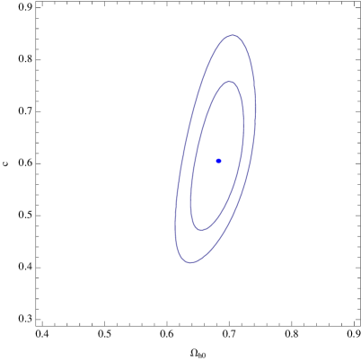
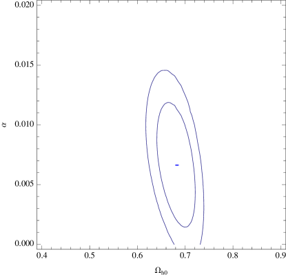
Figure 1: The contour plot of $\Omega_{h0}-c$ and $\Omega_{h0}-\alpha$ with $1\sigma,2\sigma$ confidence levels.

Current constraints ref:VG on the variation of Newton’s constant imply

$$\left|\frac{\dot{G}_{eff}}{G_{eff}}\right|\leq 10^{-11}yr^{-1},$$ (41)

in our case, which corresponds to

$$\left|\frac{\dot{\Phi}}{\Phi}\right|=\alpha H\leq 10^{-11}yr^{-1}.$$ (42)

It implies

$$\alpha\leq\frac{1}{H}\times 10^{-11}yr^{-1}.$$ (43)

Considering the current value of Hubble constant $h=0.72^{+0.08}_{-0.08}$, one obtains the bounds on $\alpha$, when the central value is taken

$$\alpha\leq 0.135807.$$ (44)

It is clear that the best fit value of parameter $\alpha$ is under the bound and consistent.

The evolution of the effective Newton’s constant is written as follows

$$\frac{G_{eff}}{G}=(1+z)^{\alpha}$$ (45)

under the assumption $\Phi/\Phi_{0}=(a/a_{0})^{\alpha}$. With the best fit value of the parameter $\alpha=0.00662$, the evolution of effective Newton’s constant with redshift $z$ is plotted in Fig. IV with the best fit parameter.

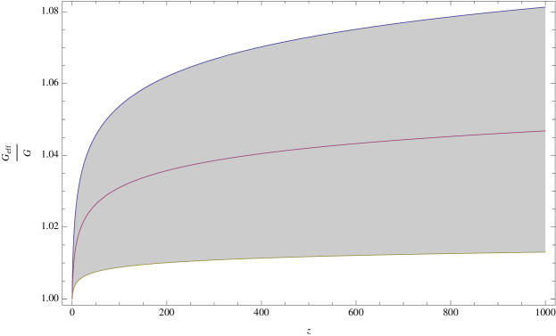
Figure 2: The evolution of effective Newton’s constant with redshift

$$z,with1\sigma regions.$$

V Conclusions

In this paper, the holographic dark energy in Brans-Dicke theory is constrained by cosmic observations which include the data sets from SN Ia, BAO and CMB shift parameter. In $1\sigma$ region, the best values of the parameters are: $\Omega_{h0}=0.683^{+0.035}_{-0.038}$, $c=0.605^{+0.138}_{-0.107}$ and $\alpha=0.00662^{+0.00477}_{-0.00467}$. Equivalently, with the relation $\omega\alpha=6$ holds, the best fit value of $\omega$ in $1\sigma$ region is $\omega=905.690^{+637.906}_{-651.471}$ which is smaller than the value from the solar system bound, but consistent with other reports in cosmological scale ref:smallomega . With these best fit values of parameters, it is found the universe is undergoing accelerated expansion currently, and the current value of equation of state of holographic dark energy $w_{h0}=-1.246^{+0.191}_{-0.144}$ which is phantom like in Brans-Dicke theory. The evolution of effective Newton’s constant is explored. Its best fit value is consistent with the bound ref:VG .

- (1) A.G. Riess, et al., Astron. J. 116 1009(1998) [astro-ph/9805201].
- (2) S. Perlmutter, et al., Astrophys. J. 517 565(1999) [astro-ph/9812133].
- (3) D.N. Spergel et.al., Astrophys. J. Supp. 148 175(2003) [astro-ph/0302209].
- (4) D.N. Spergel et al. 2006 [astro-ph/0603449].
- (5) M. Tegmark et al., Phys. Rev. D 69 (2004) 103501 [astro-ph/0310723].
- (6) M. Tegmark et al., Astrophys. J. 606 (2004) 702 [astro-ph/0310725].
- (7) I. Zlatev, L. Wang, and P.J. Steinhardt, Phys. Rev. Lett. 82 896(1999) [astro-ph/9807002].
- (8) P. J. Steinhardt, L. Wang, I. Zlatev, Phys. Rev. D59 123504(1999) [astro-ph/9812313].
- (9) M. S. Turner, Int. J. Mod. Phys. A 17S1 180(2002) [astro-ph/0202008].
- (10) V. Sahni, Class. Quant. Grav. 19 3435(2002) [astro-ph/0202076].
- (11) R. R. Caldwell, M. Kamionkowski, N. N. Weinberg, Phys. Rev. Lett. 91 071301(2003) [astro-ph/0302506].
- (12) B. Feng et al., Phys. Lett. B607 35(2005).
- (13) S. D. H. Hsu, Phys. Lett. B594 13(2004) [arXiv:hep-th/0403052].
- (14) M. Li, Phys. Lett. B603 1(2004) [hep-th/0403127].
- (15) S. Weinberg, Rev. Mod. Phys. 61 1(1989).
- (16) V. Sahni and A. A. Starobinsky, Int. J. Mod. Phys. D 9 373(2000) [arXiv:astro-ph/9904398].
- (17) S. M. Carroll, Living Rev. Rel. 4 1(2001) [arXiv:astro-ph/0004075].
- (18) P. J. E. Peebles and B. Ratra, Rev. Mod. Phys. 75 559(2003) [arXiv:astro-ph/0207347].
- (19) T. Padmanabhan, Phys. Rept. 380 235(2003) [arXiv:hep-th/0212290].
- (20) E. J. Copeland, M. Sami and S. Tsujikawa, Int. J. Mod. Phys. D 15 1753(2006) [arXiv:hep-th/0603057].
- (21) C. H. Brans and R. H. Dicke, Phys. Rev. 124 (1961) 925.
- (22) B. Bertotti, L. Iess and P. Tortora, Nature, 425, 374 (2003).
- (23) M. P. Dabrowski, T. Denkiewicz, D. Blaschke, Annalen Phys. 16, 237(2007) [arXiv:hep-th/0507068].
- (24) V. Acquaviva, L. Verde, JCAP12(2007)001, arXiv:0709.0082 [astro-ph].
- (25) C. Mathiazhagan and V. B. Johri, Class. Quantum Grav. 1 L29(1984).
- (26) D. La and P. J. Steinhardt, Phys. Rev. Lett 62 376(1989) .
- (27) S. Das, N. Banerjee, [arXiv:0803.3936].
- (28) Y. Gong, Phys. Rev. D 61 (2000) 043505;
- (29) Y. Gong, Phys. Rev. D 70 (2004) 064029, [hep-th/0404030].
- (30) M. R. Setare, Phys. Lett. B644 99(2007) [hep-th/0610190].
- (31) N. Banerjee, D. Pavon, Phys. Lett. B 647 447(2007).
- (32) B. Nayak, L. P. Singh, [arXiv:0803.2930].
- (33) L.X. Xu, W.B. Li, J.B. Lu, Eur. Phys. J. C 60 135 (2009).
- (34) V. Acquaviva, L. Verde, JCAP 0712 001(2007) [arXiv:0709.0082].
- (35) A. Riazuelo, J. Uzan, Phys.Rev. D66 023525(2002) [arXiv:astro-ph/0107386].
- (36) E. Garcia-Berro, E. Gaztanaga, J. Isern, O. Benvenuto, L. Althaus, [arXiv:astro-ph/9907440].
- (37) S. Nesseris, L. Perivolaropoulos, Phys. Rev. D73 103511(2006) [arXiv:astro-ph/0602053].
- (38) M. Kowalski et al., Astrophys. J. 686, 749(2008) [arXiv:0804.4142].
- (39) S. Nesseris and L. Perivolaropoulos, Phys. Rev. D 72, 123519 (2005) [arXiv:astro-ph/0511040]; L. Perivolaropoulos, Phys. Rev. D 71, 063503 (2005) [arXiv:astro-ph/0412308]; S. Nesseris and L. Perivolaropoulos, JCAP 0702, 025 (2007) [arXiv:astro-ph/0612653]; E. Di Pietro and J. F. Claeskens, Mon. Not. Roy. Astron. Soc. 341, 1299 (2003) [arXiv:astro-ph/0207332].
- (40) T. Okumura, T. Matsubara, D. J. Eisenstein, I. Kayo, C. Hikage, A. S. Szalay and D. P. Schneider, ApJ 676, 889(2008) [arXiv:0711.3640]
- (41) D. J. Eisenstein, et al, Astrophys. J. 633, 560 (2005) [astro-ph/0501171].
- (42) W.J. Percival, et al, Mon. Not. Roy. Astron. Soc., 381, 1053(2007) [arXiv:0705.3323]
- (43) J. R. Bond, G. Efstathiou, and M. Tegmark, MNRAS 291 L33(1997).
- (44) W. Hu, N. Sugiyama, Astrophys. J. 471 542(1996) [astro-ph/9510117].
- (45) E. Komatsu, et.al., Astrophys. J. Suppl. 180, 330(2009) [arXiv:0803.0547].
- (46) G.T. Gillies, Rep. Prog. Phys. 60, 151 (1997).