Photonic analog of graphene model and its extension
– Dirac cone, symmetry, and edge states –

Abstract

This paper presents a theoretical analysis on bulk and edge states in honeycomb lattice photonic crystals with and without time-reversal and/or space-inversion symmetries. Multiple Dirac cones are found in the photonic band structure and the mass gaps are controllable via symmetry breaking. The zigzag and armchair edges of the photonic crystals can support novel edge states that reflect the symmetries of the photonic crystals. The dispersion relation and the field configuration of the edge states are analyzed in detail in comparison to electronic edge states. Leakage of the edge states to free space is inherent in photonic systems and is fully taken into account in the analysis. A topological relation between bulk and edge, which is analogous to that found in quantum Hall systems, is also verified.

I Introduction

A mono-layer of graphite sheet, called graphene, has attracted growing interests recently.Novoselov et al. (2005); Geim and Novoselov (2007) Graphene exhibits a Dirac cone with a linear dispersion at the corner of the first Brillouin zone, resulting in a variety of novel transport phenomena of electrons. They stimulate theoretical and experimental studies taking account of analogy to physics of relativistic electron, such as Klein tunnelingKlein (1929) and ZitterbewegungSchrodinger (1930). Moreover, semi-infinite graphene and finite stripe of graphene with zigzag edges support a novel edge state with nearly flat dispersion.Nakada et al. (1996) On the contrary, armchair edge does not support such an edge state. The flat dispersion implies that the density of state (DOS) diverges at the flat band energy, in a striking contrast to the zero DOS in bulk. So far, theoretical investigation of graphene heavily relies on the tight-binding model. It is not clear to what extent the edge states change in other models on the honeycomb lattice.

Here, we study a photonic analog of graphene model,Cassagne et al. (1995) namely, two-dimensional photonic crystal (PhC) composed of the honeycomb lattice of dielectric cylinders embedded in a background substance. The honeycomb lattice consists of two inter-penetrating triangular lattices (called A and B sub-lattices) with the same lattice constant. In PhC it is not rare to have the Dirac cone in the dispersion diagram. Triangular and honeycomb lattices of identical circular rods support multiple Dirac cones at the corner of the first Brillouin zone. It should be noted that they have the same point group of six-fold symmetry. Doubly degenerate modes at the corner of the first Brillouin zone exhibit the Dirac cone owing to the point group symmetry.Chong et al. (2008) This fact suggests that, the symmetry is crucial and the Dirac cone is not limited in the tight-binding model of electrons on the honeycomb lattice.

Some perturbation breaks the symmetry of the original honeycomb lattice and causes a crucial influence on the linear dispersion. In electronic systems the energy difference between A- and B-site atomic orbitals,Semenoff (1984) periodic magnetic flux of zero average,Haldane (1988) and Rashba spin-orbit interactionKane and Mele (2005) are such examples of the symmetry breaking. They break at least either of time-reversal symmetry (TRS) or space-inversion symmetry (SIS) or parities in plane. Therefore, the point group of the original honeycomb lattice is reduced into a smaller group. As a result, the two-dimensional irreducible representations are prohibited, and the doubly-degenerate modes are lifted. The gap between the lifted modes is correlated with the magnitude of the symmetry breaking. The effective theory around a nearly degenerate point is described by the massive Dirac Hamiltonian, where the mass gap can be controlled via the degree of the symmetry breaking.

In the honeycomb lattice PhCs the TRS is efficiently broken by applying a magnetic field parallel to the cylindrical axis. Nonzero static magnetic field induces imaginary off-diagonal elements in the permittivity or permeability tensors, through the magneto-optical effect. The SIS is broken if the A-site rods are different from the B-site rods.Onoda and Ochiai Therefore, we can continuously tune the degree of the symmetry breaking in the honeycomb lattice PhCs. This tunability is a great advantage of the photonic analog of graphene model and its extension.Haldane (1988) From a theoretical point of view, the tight-binding approximation, which is commonly used in modeling of graphene, is not widely applicable for photonic band calculation. Accordingly, the non-bonding orbital in the nearest neighbor tight-binding approximation, which is responsible for flatness of the dispersion curve of the zigzag edge state, is completely absent in PhCs. For example, even in the original honeycomb PhC with both the TRS and the SIS, the dispersion of the zigzag edge states is not flat because of the absence of the non-bonding orbital.

Regarding the system with boundary, photonic system is quite distinct from electronic system. In the latter system the electrons near Fermi level are prohibited to escape to the outer region via the work function, i.e., a confining potential, and the wave functions of the electrons are evanescent in the outer region. Therefore, to sustain an edge state, formation of the band gap in bulk is the minimum requirement. On the other hand, in the former system confining potentials for photon are absent at the boundary. Energy of photon is always positive as in free space, and no energy barrier exists between the PhC and free space. The simplest way to confine photonic edge states in the PhC is to utilize the light cone. This restriction of the confinement makes photonic systems quit nontrivial in various aspects. In particular, the topological relation between bulk and edgeHatsugai (1993) is of high interest in photonic systems without TRS. In quantum Hall system nontrivial topology of bulk states leads to the emergence of chiral edge states, which are robust against localization effect. The edge states play a crucial role in this system.Halperin (1982); Wen (1991) Recently, Haldane and Raghu proposed one-way light waveguide realized in PhCs without TRS.Haldane and Raghu (2008) Explicit construction of such waveguides is demonstrated by several authors.Wang et al. (2008); Yu et al. (2008); Raghu and Haldane (2008); Takeda and John (2008) This paper also shades light to this topic, by using simpler structure than those demonstrated so far.

This paper is organized as follows. Section II is devoted to present bulk properties of the PhC with and/or without TRS and SIS. A numerical method to deal with edge states is given in Sec. III. Properties of zigzag and armchair edge states are investigated in detail in Secs. IV and V, respectively. A one-way light transport along the edge of a rectangular-shaped PhC is demonstrated in Sec. VI. Finally, summary and discussions are given in Sec. VII.

II Dirac cone and band gap

Let us consider two-dimensional PhCs composed of the honeycomb array of circular cylinders embedded in air. The photonic band structure of the PhCs with and without TRS is shown in Fig. 1 for the transverse magnetic (TM) polarization. For comparison, the photonic band structure of the transverse electric (TE) polarization is also shown for the PhC with TRS. The SIS holds in all the cases.

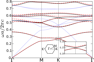
Figure 1: (Color online) The photonic band structure of the honeycomb lattice PhCs of dielectric cylinders embedded in air. Solid (dashed) line stands for the TM band structure of the PhC with (without) TRS. The SIS holds in both the cases. The dielectric constant and radius of the cylinders are taken to be 12 and $0.2a$, respectively, where $a$ is the lattice constant. The magnetic permeability of the cylinders is taken to be 1 for the PhC with TRS and is given by Eq. (4) for the PhC without TRS. For comparison, the TE band structure of the PhC with TRS is shown by doted line.

Here, the dielectric constants $\varepsilon_{A(B)}$ and radius $r_{A(B)}$ of the A(B)-cylinders are taken to be 12 and $0.2a$, respectively. The magnetic permeability of the cylinders is taken to be 1 for the PhC with TRS, and has the tensor form given by

$$\hat{\mu}=\left(\begin{array}[]{ccc}\mu&i\kappa&0\\ -i\kappa&\mu&0\\ 0&0&\mu\end{array}\right),\quad\mu=1,\quad\kappa=0.2,$$ (4)

for the PhC without TRS. The first, second, and third rows (columns) stand for $x,y$ and $z$ Cartesian components, respectively. The cylindrical axis is taken to be parallel to the $z$ axis. The imaginary off-diagonal components of $\hat{\mu}$ are responsible for the magneto-optical effect and break the TRS. Thus, parameter $\kappa$ represents the degree of the TRS breaking.

As mentioned in Introduction, for the PhC with TRS the Dirac cone is found at the K point. In particular, the first (lowest) and second TM bands are in contact with each other at the K point. They are also in contact with the K’ point because of the spatial symmetry. This property is quite similar to the tight-binding electron in graphene. As for the Dirac point at $\omega a/2\pi c\simeq 0.55$ of the TM polarization, the fourth band is in contact with the fifth band at K (and K’), whereas the former and the latter are also in contact with the third and sixth bands, respectively at the $\Gamma$ point. Concerning the TE polarization, the Dirac cones are not clearly visible, but are indeed formed between the second and third and between the fourth and fifth.

On the other hand, in the PhC without TRS, all the degenerate modes at $\Gamma$ and K are lifted. The point group of this PhC becomes $C_{6}$ and the point group of ${\boldsymbol{k}}$ at the K point is $C_{3}$. They are abelian groups, allowing solely one-dimensional representations. Therefore, the degeneracy is forbidden. The energy gap between the lifted modes is proportional to $\kappa$ if it is small enough. The SIS breaking, $\Delta\varepsilon=\varepsilon_{A}-\varepsilon_{B}$, lifts the double degeneracy at K, but not at $\Gamma$ when the TRS is preserved. The energy gap between the lifted modes is proportional to $\Delta\varepsilon$.Onoda and Ochiai

Let us focus on the gap between the first and second TM bands of the PhC as a function of the SIS and TRS breaking parameters. The phase diagram of the PhC concerning the gap is shown in Fig. 2.

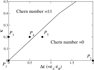
Figure 2: Phase diagram of the honeycomb lattice PhCs for the TM polarization. Phase space is spanned by two parameters, $\Delta\epsilon$ and $\kappa$, which represent the SIS and TRS breaking, respectively. The average dielectric constant and the radius of the cylinders are kept fixed to $(\varepsilon_{A}+\varepsilon_{B})/2=12$ and $r_{A}=r_{B}=0.2a$, respectively.

At generic values of the parameters the gap opens. However, if we change the parameters along a certain curve in the parameter space, the gap remains to close as shown in Fig. 2. This property implies that at finite $\kappa$ the gap closes only at a certain value of $\Delta\varepsilon$. Although the gap opens in both the regions above and below the curve, the two regions are topologically different, and are characterized by the Chern numbers of the first and second photonic bands. The Chern number is a topological integer defined by

$$C_{n}=\frac{1}{2\pi}\int_{\rm BZ}d^{2}k(\nabla_{\boldsymbol{k}}\times{\boldsymbol{\Lambda}}_{n{\boldsymbol{k}}})_{z},$$ (5)

$${\boldsymbol{\Lambda}}_{n{\boldsymbol{k}}}=-i\langle u_{n{\boldsymbol{k}}}|\nabla_{\boldsymbol{k}}|u_{n{\boldsymbol{k}}}\rangle,$$ (6)

$$\langle u_{m{\boldsymbol{k}}}|u_{n{\boldsymbol{k}}}\rangle=\frac{1}{A}\int_{\rm UC}d^{2}xu_{m{\boldsymbol{k}}}({\boldsymbol{x}})\varepsilon({\boldsymbol{x}})u_{n{\boldsymbol{k}}}({\boldsymbol{x}})=\delta_{m,n}$$ (7)

for each non-degenerate band. Here, BZ, UC, and $A$ stand for Brillouin zone, unit cell, and the area of unit cell, respectively. The envelop function $u_{n{\boldsymbol{k}}}({\boldsymbol{x}})$ of the $n$-th Bloch state at ${\boldsymbol{k}}$ is of $E_{z}$ (i.e., the $z$ component of the electric field). In the upper region of Fig. 2, $C_{1}=-1$ and $C_{2}=1$, whereas in the lower region $C_{1}=C_{2}=0$. At the gap closing point, the Chern number transfers between the upper and lower band under the topological number conservation law.Avron et al. (1983) We will see that the phase diagram correlates with a property of edge states in corresponding PhC stripes. This correlation is a guiding principle to design a one-way light transport near PhC edges.Haldane and Raghu (2008)

Figure 2 shows solely the phase diagram in the first quadrant of real $\Delta\varepsilon$ and $\kappa$. The mirror reflection with respect to the $\Delta\varepsilon$ axis gives the phase diagram in the fourth quadrant, where $C_{1}$ and $C_{2}$ are interchanged due to the inversion of $\kappa$. The phase diagram in the second and third quadrants is obtained by the mirror reflection with respect to the $\kappa$ axis. The resulting phase diagram is similar to that obtained in a triangular lattice PhC with anisotropic rods.Raghu and Haldane (2008)

III characterization of edge states

So far, we have concentrated on properties of the PhCs of infinite extent in plane. If the system has edges, there can emerge edge states which are localized near the edges and are evanescent both inside and outside the PhC. In this section we introduce a PhC stripe with two parallel boundaries. The boundaries are supposed to have infinite extent, so that the translational invariance along the boundary still holds. The edge states are characterized by Bloch wave vector parallel to the boundary.

Optical properties of the PhC stripe are described by the S-matrix. It relates the incident plane wave of parallel momentum $k_{\|}+G^{\prime}$ to the outgoing plane wave of parallel momentum $k_{\|}+G$, where $G$ and $G^{\prime}$ are the reciprocal lattice vectors relevant to the periodicity parallel to the stripe.Pendry (1974) Both the waves can be evanescent. To be precise, the S-matrix is defined by

$$\left(\begin{array}[]{c}(a_{+}^{\rm out})_{G}\\ (a_{-}^{\rm out})_{G}\end{array}\right)=\sum_{G^{\prime}}\left(\begin{array}[]{cc}(S_{++})_{GG^{\prime}}&(S_{+-})_{GG^{\prime}}\\ (S_{-+})_{GG^{\prime}}&(S_{--})_{GG^{\prime}}\end{array}\right)\left(\begin{array}[]{c}(a_{+}^{\rm in})_{G^{\prime}}\\ (a_{-}^{\rm in})_{G^{\prime}}\end{array}\right),$$ (14)

where $(a_{\pm}^{\rm in(out)})_{G}$ is the plane-wave-expansion components of upward (+) and downward (-) incoming (outgoing) waves of parallel momentum $k_{\|}+G$, respectively. In our PhCs under consideration the S-matrix can be calculated via the photonic layer-Korringa-Kohn-Rostoker methodOhtaka et al. (1998) as a function of parallel momentum $k_{\|}$ and frequency $\omega$. If the S-matrix is numerically available, the dispersion relation of the edge states is obtained according to the following secular equation:

$$0={\rm det}[S^{-1}].$$ (15)

Strictly speaking, this equation also includes solutions of bulk states below the light line. If we search for the solutions inside pseudo gaps (i.e. $k_{\|}$-dependent gaps), solely the dispersion relations of the edge states are obtained. In actual calculation, however, the magnitude of ${\rm det}[S]$ becomes extremely small with increasing size of the matrix. The matrix size is given by the number of reciprocal lattice vectors taken into account in numerical calculation. In order to obtain numerical accuracy, we have to deal with larger matrix. Therefore, this procedure to determine the edge states is generally unstable. Instead, we employ the following scheme. Suppose that the S-matrix is divided into two parts $S^{u}$ and $S^{l}$ that correspond to the division of the PhC stripe into the upper and lower parts. This division is arbitrary, unless the upper or lower part is not empty. The following secular equation also determines the dispersion relation of the edge states:

$$0={\rm det}[1-S_{-+}^{l}S_{+-}^{u}].$$ (16)

This scheme is much stable for larger matrix.

As far as true edge states are concerned, the secular equation has the zeros in real axis of frequency for a given real $k_{\|}$. Here we should also mention leaky edge states (i.e., resonances near the edges), which are not evanescent outside the PhC but are evanescent inside the PhC. Such an edge state is still meaningful, because the DOS exhibits a peak there. The peak frequency as a function of parallel momentum $k_{\|}$ follows a certain curve that is connected to the dispersion curve of the true edge states. To evaluate the leaky edge states, the method developed by Ohtaka et alOhtaka et al. (2004) is employed. In this method, the DOS at fixed $k_{\|}$ and $\omega$ is calculated with the truncated S-matrix of open diffraction channels. The unitarity of the truncated S-matrix enables us to determine the DOS via eigen-phase-shifts of the S-matrix. A peak of the DOS inside the pseudo gap corresponds to a leaky edge state.

IV zigzag edge

First, let us consider the zigzag edge. Figure 3 shows four sets of the projected band diagram of the honeycomb PhC and the dispersion relation of the edge states localized near the zigzag edges. In Fig. 3 the shaded regions represent bulk states, whereas the blank regions correspond to the pseudo gap. Inside the pseudo gap edge states can emerge. In the evaluation of the edge states, we assumed the PhC stripe of $N=16$, being $N$ the number of the layers along the direction perpendicular to the zigzag edges.

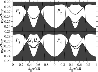
Figure 3: The projected band diagrams at point $P_{n}$ in the phase diagram (Fig. 2) and the dispersion curves of the edge states. The zigzag edge is assumed. The shaded regions represent bulk states. The edge states are of the PhC stripes with 16 layers. Thin solid line stands for the light line. The surface Brillouin zone is taken to be $0\leq k_{\|}a/2\pi\leq 1$ in order to see the connectivity of the edge-state dispersion curves.

Here, we close up the first and second bands. Higher bands are well separated from the lowest two bands. Each set refers to either of four points indicated in the phase diagram of Fig. 2. In accordance with the Dirac cone in Fig. 1, the projected band structure of point $P_{1}$ also exhibits a point contact at $k_{\|}a/2\pi=1/3$ and $2/3$. The first and second bands are separated for $P_{2}$ and $P_{3}$, but are nearly in contact at $k_{\|}a/2\pi=1/3$ for $P_{4}$. This is because $P_{4}$ is close to the phase boundary. Except for the lower right panel, in which the TRS and the SIS are broken, the projected band diagrams and the edge-state dispersion curves are symmetric with respect to $k_{\|}a/2\pi=0.5$. This symmetry is preserved if either the TRS or the SIS holds. The time-reversal transformation implies

$$\omega_{n}(-k_{\|},-k_{\perp};\Delta\varepsilon,-\kappa)=\omega_{n}(k_{\|},k_{\perp};\Delta\varepsilon,\kappa),$$ (17)

where $\omega_{n}(k_{\|},k_{\perp};\Delta\varepsilon,\kappa)$ is the eigen-frequency of the $n$-th Bloch state at given parameters of $\Delta\varepsilon$ and $\kappa$, and $k_{\perp}$ is the momentum perpendicular to the edge. Since $\kappa$ is inverted, Eq. (17) is not a symmetry of the PhC, but is just a transformation law. In the case of $\kappa=0$, after the projection concerning $k_{\perp}$, the symmetry with respect to $k_{\|}=0$ is obtained. This symmetry combined with the translational invariance under $k_{\|}\to k_{\|}+G$ results in the symmetry with respect to $k_{\|}a/2\pi=0.5$. Similarly, the space inversion results in

$$\omega_{n}(-k_{\|},-k_{\perp};-\Delta\varepsilon,\kappa)=\omega_{n}(k_{\|},k_{\perp};\Delta\varepsilon,\kappa).$$ (18)

The symmetry with respect to $k_{\|}a/2\pi=0$ and $0.5$ is obtained at $\Delta\varepsilon=0$.

When edge states are well defined in PhCs with enough number of layers, their dispersion relation satisfies

$$\omega_{e_{1}(e_{2})}(-k_{\|};\Delta\varepsilon,-\kappa)=\omega_{e_{1}(e_{2})}(k_{\|};\Delta\varepsilon,\kappa),$$ (19)

$$\omega_{e_{1}}(-k_{\|};-\Delta\varepsilon,\kappa)=\omega_{e_{2}}(k_{\|};\Delta\varepsilon,\kappa),$$ (20)

owing to the time-reversal and space-inversion transformations, respectively. Here, $\omega_{e_{1}}$ and $\omega_{e_{2}}$ denote the dispersion relation of opposite edges of the PhC stripe. At $\kappa=0$, both $\omega_{e_{1}}$ and $\omega_{e_{2}}$ are symmetric under the inversion of $k_{\|}$. In contrast, at $\Delta\varepsilon=0$ they are interchanged. The resulting band diagram is symmetric with respect to $k_{\|}a/2\pi=0$ and $0.5$ as in Fig. 3.

The upper left panel of Fig. 3 shows two almost-degenerate curves that are lifted a bit near the Dirac point. This lifting comes from the hybridization between edge states of the opposite boundary, owing to finite width of the stripe. The lifting becomes smaller with increasing $N$, and eventually two curves merge with each other. Since $P_{1}$ corresponds to $\Delta\varepsilon=\kappa=0$, we obtain $\omega_{e1}=\omega_{e2}$ owing to Eqs. (19) and (20), irrespective of $k_{\|}$. As is the same with in graphene, our edge states appear only in the region $1/3\leq k_{\|}a/2\pi\leq 2/3$. However, the edge-state curves are not flat, in a striking contrast to the zigzag edge state in the nearest-neighbor tight-binding model of graphene.

In the upper right panel two edge-state curves are separated in frequency and each curve terminates in the same bulk band. On the contrary, in the lower two panels the dispersion curves of the two edge states intersect one another at a particular point and each curve terminates at different bulk bands. For instance, in the lower left panel, the curve including $Q_{1}$ terminates at the upper band near $k_{\|}a/2\pi=1/3$ and at the lower band near $k_{\|}a/2\pi=2/3$. At other points in the parameter space, we found that the two edge-state curves are separated if the system is in the phase of zero Chern number. Otherwise, if the system is in the phase of non-zero Chern number, the two curves intersect one another.

The wave function of the edge state at marked points $Q_{1}$ and $Q_{2}$ is plotted in Fig. 4.

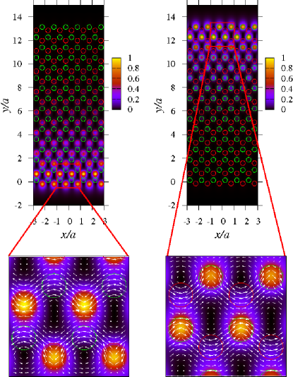
Figure 4: (Color online) The electric field intensity $|E_{z}|^{2}$ of the true edge state at $Q_{1}$ (left panel) and $Q_{2}$ (right panel) in Fig. 3. The intensity maxima is normalized as 1. In the enlarged panels the Poynting vector flow is also shown.

We can easily see that the edge states at $Q_{1}$ and $Q_{2}$ are localized near different edges. This property is consistent with the fact that at $\Delta\varepsilon=0$, $\omega_{e_{1}}$ and $\omega_{e_{2}}$ are interchanged under the inversion of $k_{\|}$. The field configuration at $Q_{1}$ is identical to that at $Q_{2}$ after the space-inversion operation ($\pi$ rotation). Since the SIS is preserved in this case, they are the SIS partners. It is also remarkable that the electric field intensity is confined almost in the rods forming one particular sub-lattice. This field pattern is reminiscent of the non-bonding orbital of the zigzag edge state in graphene. The edge state at $Q_{1}(Q_{2})$ has the negative (positive) group velocity. Moreover, no other bulk and edge states exist at the frequency. Therefore, solely the propagation from left to right is allowed near the upper edge, while the propagation from left to right is allowed in the lower edge. In this way a one-way light transport is realized near a given edge. The one-way transport is robust against quenched disorder with long correlation length, because the edge states are out of the light line and the bulk states at the same frequency is completely absent.Ono et al. (1989) This is also the case in the lower right panel of Fig. 3, although the frequency range of the one-way transport is very narrow. It should be noted that the non-correlated disorder would cause the scattering into the states above the light line, where the energy leakage takes place. Detailed investigation of disorder effects is beyond the scope of the present paper.

The results obtained in this section strongly support the bulk-edge correspondence, which was originally proven in the context of quantum Hall systemsHatsugai (1993) and was discussed in the context of photonic systems recently.Haldane and Raghu (2008) Namely, the number of one-way edge states in a given two-dimensional omni-directional gap (i.e. $k_{\|}$-independent gap) is equal to the sum of the Chern numbers of the bulk bands below the gap. In our case the Chern number of the lower (upper) band is equal to -1 (1). A negative sign of the sum corresponds to the inverted direction of the edge propagation. Accordingly, there is only one (one-way) state per edge in the gap between the first and second bands. Moreover, no edge state is found between the second and third bands. This behavior is consistent with the Chern numbers of the first and second bands, according to the bulk-edge correspondence.

Finally, let us briefly comment on the edge states in $P_{1}$ and $P_{2}$. In $P_{1}$ the two edge states are completely degenerate at $N=\infty$. For the system with narrow width, there appear the bonding and anti-bonding orbitals, each of which has an equal weight of the field intensity in both the zigzag edges. As for the edge states in $P_{2}$, the upper (lower) edge states are localized near the upper (lower) zigzag edge.

V armchair edge

Next, let us consider the armchair edge. The projected band diagram and the dispersion curves of the edge states are shown in Fig. 5. We assumed the PhC stripe with $N=64$.

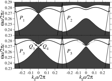
Figure 5: The projected band diagrams at point $P_{n}$ in the phase diagram (Fig. 2) and the dispersion curves of the edge states. The armchair edge is assumed. The shaded regions correspond to bulk states. The edge states are of the PhC stripes with 64 layers. Thin solid line stands for the light line.

It should be noted that they are symmetric with respect to $k_{\|}=0$ regardless of SIS and TRS. This property is understood by the combination of a parity transformation and Eq. (17). Under the parity transformation with respect to the mirror plane parallel to the armchair edges,

$$\omega_{n}(k_{\|},-k_{\perp};\Delta\varepsilon,-\kappa)=\omega_{n}(k_{\|},k_{\perp};\Delta\varepsilon,\kappa).$$ (21)

By combining Eqs. (17) and (21), we obtain the symmetric projected band diagram with respect to $k_{\|}=0$. Concerning the edge states, the parity transformation results in

$$\omega_{e_{1}}(k_{\|};\Delta\varepsilon,-\kappa)=\omega_{e_{2}}(k_{\|};\Delta\varepsilon,\kappa).$$ (22)

Therefore, by combining Eqs. (19) and (22), we can derive that $\omega_{e_{1}}$ and $\omega_{e_{2}}$ are interchanged by the inversion of $k_{\|}$, regardless of SIS and TRS:

$$\omega_{e_{1}}(-k_{\|};\Delta\varepsilon,\kappa)=\omega_{e_{2}}(k_{\|};\Delta\varepsilon,\kappa).$$ (23)

Equation (23) results in the degeneracy between $\omega_{e_{1}}$ and $\omega_{e_{2}}$ at the boundary of the surface Brillouin zone. Moreover, it is obvious from Eq. (22) that the two edge states are completely degenerate at $\kappa=0$ in the entire surface Brillouin zone.

In the armchair projection the K and K’ points in the first Brillouin zone are mapped on the same point $k_{\|}=0$ in the surface Brillouin zone, being above the light line. Therefore, possible edge states relevant to the Dirac cone are leaky, unless the region outside the PhC is screened. Accordingly, the DOS of an armchair edge state at fixed $k_{\|}$ shows up as a Lorentzian peak, in a striking contrast to that of a zigzag edge state being a delta-function peak. The dispersion relation of the leaky edge states depends strongly on the number of layers $N$. However, if $N$ is large enough, the $N$-dependence disappears. We found that at large enough $N$, the leaky edge states correlate with the Chern number fairly well.

In the case as $P_{3}$ where the Chern numbers of the upper and lower bands are nonzero, we found a segment of the dispersion curve of the leaky edge state whose bottom is at the lower band edge, as shown in the lower left panel of Fig. 5. There also appear another segment of the dispersion curve which crosses the light line. Across the phase boundary, the upper band touches to and separates from the lower band. After the separation as the case $P_{5}$, the bottom of the former segment moves from the lower band edge to the upper band edge as shown in the lower right panel of Fig. 5. By increasing $\Delta\varepsilon$, this segment hides among the upper bulk band (not shown). We should note that the dispersion curve of the leaky edge states is obtained by tracing the peak frequencies of the DOS as a function of $k_{\|}$. If a peak becomes a shoulder, we stopped tracing the curve and indicated shoulder frequencies by dotted curve. This is the case for $P_{3}$ and $P_{5}$. For $P_{3}$, the DOS changes its shape from peak to shoulder at $k_{\|}a/2\pi\simeq\pm 0.058$. This is why the segment including $Q_{3}$ and $Q_{4}$ seems to terminate around there. However, we can distinguish this shoulder in the region $0.058<|k_{\|}|a/2\pi<0.1$, accompanying an additional peak above it. The peak bringing the shoulder with it becomes an asymmetric peak for $|k_{\|}|a/2\pi>0.1$ and crosses the light line. In the DOS spectrum of $P_{5}$, we can find two shoulders just below the peaks of bulk states in the region $0.04<|k_{\|}|a/2\pi<0.1$. Again, they merge each other and become an asymmetric peak for $|k_{\|}|a/2\pi>0.1$. Such an asymmetric peak consists of two peaks with different heights and widths, which come from the lifting of the degenerate edge states in the limit of $\kappa=0$. Actually, for $P_{1}$ and $P_{2}$ in which the edge states are doubly-degenerate, we can see a nearly-symmetric single peak for the leaky edge states in each case.

As in the case of zigzag edge, the leaky edge states in the two-dimensional omni-directional gap exhibit a one-way light transport if the relevant Chern number is nonzero. Here, we consider the structure with two horizontal armchair edges. The incident wave with positive $k_{\|}$ coming from the bottom cannot excite the leaky edge state just above the lower band edge, e.g., state $Q_{4}$ in Fig. 5. However, the incident wave with negative $k_{\|}$ coming from the bottom can excite the leaky edge state, e.g., at $Q_{3}$. In the latter case, the leaky edge state has negative group velocity, traveling from right to left. This relation becomes inverted for the plane wave coming from the top. The incident plane wave with positive (negative) $k_{\|}$ can (cannot) excite the leaky edge state localized near the upper armchair edge. This edge state has positive group velocity, traveling from left to right. In this way, one-way light transport is realized as in the zigzag edge case. Under quenched disorder the one-way transport is protected against the mixing with bulk states, because no bulk state exists in the omni-directional gap. However, in contrast to the zigzag edge case, even the disorder with long correlation length could enhance the energy leakage to the outer region.

Figure 6 shows the electric field intensity $|E_{z}|^{2}$ induced by the incident plane wave whose $\omega$ and $k_{\|}$ are at the marked points ($Q_{3}$ and $Q_{4}$) in Fig. 5. The intensity of the incident plane wave is taken to be 1 and the field configuration above $y/a=8$ is omitted.

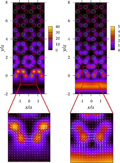
Figure 6: (Color online) The electric field intensity $|E_{z}|^{2}$ induced by the incident plane wave having $(k_{\|},\omega)$ at $Q_{3}$ (left panel) and $Q_{4}$ (right panel) in Fig. 5. The incident plane wave of unit intensity comes from the bottom of the structure. In the enlarged panels the Poynting vector flow is also shown.

Although, the dispersion curve is symmetric with respect to $k_{\|}=0$, the field configuration is quite asymmetric. Of particular importance is the near-field pattern around the lower edge. In the left panel the strongest field intensity of order 40 is found in the boundary armchair layer, whereas in the right panel it is found outside the PhC with much smaller intensity. In both the cases, the transmittances are the same and nearly equal to zero. Accordingly, no field enhancement is observed near the upper edge (not shown). The remarkable contrast of the field profiles indicates that the leaky edge state with horizontal energy flow is excited in the left panel, but is not in the right panel. If the plane wave is incident from the top, the field pattern exhibits an opposite behavior. That is, the plane wave with $\omega$ and $k_{\|}$ at $Q_{4}$ from the top excites the leaky edge state localized near the upper edge, but at $Q_{3}$ it cannot excite the leaky edge state.

The property of each edge state is also understood as follows. When we scan $k_{\|}$ from negative to positive along the dispersion curve of the leaky edge state, the localized center of the edge state transfers from one edge to the other. The critical point is at the bottom of the dispersion curve, where the edge state merges to the bulk state of the lower band. It is extended inside the PhC, making a bridge from one edge to the other. The entire picture is consistent with the interchange of $\omega_{e_{1}}$ and $\omega_{e2}$ under the inversion of $k_{\|}$.

Finally, let us comment on the field configuration of other edge states. For $P_{1}$ and $P_{2}$, the edge states are degenerate between the upper and lower edges. Accordingly, the incident plane wave coming from the bottom (top) of the structure excites the leaky edge states localized around the bottom (top) edge. It is regardless of the sign of $k_{\|}$. For $P_{3}$ and $P_{5}$, the edge-state curve that crosses the light line corresponds to an asymmetric peak in the DOS, which is actually the sum of two peaks. It is difficult to separate the two peaks, because they are overlapped in frequency. Thus, the edge states can be excited by the incident wave coming from both top and bottom of the PhC. Concerning the quadratic edge state around $k_{\|}=0$ of $P_{5}$, a similar contrast in the field configuration between positive and negative $k_{\|}$ is obtained as in $Q_{3}$ and $Q_{4}$. However, under quenched disorder this edge state readily mixes with bulk states that exist at the same frequency.

VI Demonstration of one-way light transport

The direction of the one-way transport in the zigzag edge is consistent with that in the armchair edge. Let us consider a rectangular-shaped PhC whose four edges are zigzag, armchair, zigzag, and armchair in a clockwise order. The one-way transport found in Figs. 3 and 5 must be clockwise in this geometry.

To verify it certainly happens, we performed a numerical simulation of the light transport in the rectangular-shaped PhC. The multiple-scattering method is employed along with a Gaussian beam incidence.Bravo-Abad et al. (2003) We assume $N=32$ for the zigzag edges and $N=64$ for the armchair edges. The incident Gaussian beam is focused at the midpoint of the front armchair edge. The electric field intensity $|E_{z}|^{2}$ at the focused point is normalized as 1 and the beam waist is $10a$. The frequency and the incident angle of the beam are taken to be $\omega a/2\pi c=0.273$ and $\theta_{0}=7.263^{\circ}$, which corresponds to the leaky edge state very close to the $Q_{3}$ point. The beam waist size is chosen to avoid possible diffraction at the corner of the PhC and not to excite the states near the $Q_{4}$ point at the same time.

Resulting electric field intensity $|E_{z}|^{2}$ is plotted in Fig. 7.

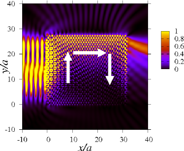
Figure 7: (Color online) The electric field intensity $|E_{z}|^{2}$ induced by the time-harmonic Gaussian beam coming from the left of the rectangular-shaped PhC. The four edges are either zigzag (top and bottom) or armchair (left and right). The beam is focused at the mid point of the left armchair edge with the unit electric field intensity and beam waist of $10a$.

The incident beam is almost reflected at the left (armchair) edge, forming the interference pattern in the left side of the PhC. However, as in the left panel of Fig. 6, the leaky edge state is certainly excited there. This edge state propagates upward, and is diffracted at the upper left corner. A certain portion of the energy turns into the zigzag edge state localized near the upper edge. This edge state propagates from left to right. The energy leakage at the upper edge is very small compared to that in the left and right edges. This zigzag edge state is more or less diffracted at the upper right corner. However, the down-going armchair edge state is certainly excited in the right edge. Obviously, the field intensity of the right edge reduces with reducing $y$ coordinate. This behavior is consistent with the energy leakage of the armchair edge state. Finally, the field intensity almost vanished at the lower right corner. In this way, the clockwise one-way light transport is realized in the rectangular-shaped PhC.

We also confirmed that the incident beam with the same parameters but inverted incident angle ($-\theta_{0}$) does not excite the counterclockwise one-way transport along the edges. The incident beam is just reflected without exciting the relevant leaky edge state in accordance with the right panel of Fig. 6.

VII Summary and discussions

In summary, we have presented a numerical analysis on the bulk and edge states in honeycomb lattice PhCs as a photonic analog of graphene model and its extension. In the TM polarization the Dirac cone emerges between the first and second bands. The mass gap in the Dirac cone is controllable by the parameters of the SIS or TRS breaking. On a certain curve in the parameter space, the band touching takes place. This curve divides the parameter space into two topologically-distinct regions. One is characterized by zero Chern number of the upper and lower bands, and the other is characterized by Chern number of $\pm 1$. Of particular importance is the correlation between the Chern number in bulk and light transport near edge. Non-zero Chern number in bulk photonic bands results in one-way light transport near the edge. It is quite similar to the bulk-edge correspondence found in quantum Hall systems.

In this paper we focus on the TM polarization in rod-in-air type PhCs. This is mainly because the band touching takes place between the lowest two bands and they are well separated from higher bands by the wide band gap, provided that the refractive index of the rods are high enough. In rod-in-air type PhCs the TE polarization results in the band touching between the second and third bands. However, the Dirac cone is not clearly visible, although it is certainly formed. As for hole-in-dielectric type PhCs, an opposite tendency is found. Namely, the band touching between the lowest two bands takes place only in the TE polarization. In this case the distance between the boundary column of air holes and the PhC edge affect edge states. Therefore, we must take account of this parameter to determine the dispersion curves of the edge states.

Concerning the TRS breaking, we have introduced imaginary off-diagonal components in the permeability tensor. This is the most efficient way to break the TRS for the TM polarization. Such a permeability tensor is normally not available in visible frequency range.Landau et al. (1985) However, in GHz range it is possible to obtain $\kappa$ of order 10. Such a large $\kappa$ is necessary to obtain a robust one-way transport against thermal fluctuations, etc. In the numerical setup we assume an intermediate frequency range with smaller $\kappa$. On the other hand, in the TE polarization, the TRS can be efficiently broken by imaginary off-diagonal components in the permittivity tensor. In this case the PhC without the TRS can operate in visible frequency range. However, strong magnetic field is necessary in order to induce large imaginary off-diagonal components of the permittivity tensor. Thus, it is strongly desired to explorer low-loss optical media with large magneto-optical effect, in order to have robust one-way transport.

Recently, another photonic analog of graphene, namely, honeycomb array of metallic nano-particles, is proposed and analyzed theoretically.Han et al. (2009) Particle plasmon resonances in the nano-particles act as if localized orbitals in Carbon atom. The tight-binding picture is thus reasonably adapted to this system, and nearly flat bands are found in the zigzag edge. Vectorial nature of photon plays a crucial role there, giving rise to a remarkable feature in the dispersion curves of the edge states in the quasi-static approximation. In contrast, vectorial nature of photon is minimally introduced in our model, but a full analysis including possible retardation effects and symmetry-breaking effects has been made. Effects of the TE-TM mixing in off-axis propagation are an important issue in our system. In particular, it is interesting to study to what extent the bulk-edge correspondence is modified. We hope this paper stimulates further investigation based on the analogy between electronic and photonic systems on honeycomb lattices.