Distributed Discovery of Large Near-Cliques

Given an undirected graph and $0\leq\epsilon\leq 1$, a set of nodes is called $\epsilon$-near clique if all but an $\epsilon$ fraction of the pairs of nodes in the set have a link between them. In this paper we present a fast synchronous network algorithm that uses small messages and finds a near-clique. Specifically, we present a constant-time algorithm that finds, with constant probability of success, a linear size $\epsilon$-near clique if there exists an $\epsilon^{3}$-near clique of linear size in the graph. The algorithm uses messages of $O(\log n)$ bits. The failure probability can be reduced to $n^{-\Omega(1)}$ in $O(\log n)$ time, and the algorithm also works if the graph contains a clique of size $\Omega(n/\log^{\alpha}\log n)$ for some $\alpha\in(0,1)$. Our approach is based on a new idea of adapting property testing algorithms to the distributed setting.

1 Introduction

Discovering dense subgraphs is an important task both theoretically and practically. From the theoretical point of view, clique detection is a fundamental problem in the theory of computational complexity, and for distributed algorithms, computing useful constructs of the underlying communication graph is one of the central goals. Let us elaborate a little about that.

Dense graph detection has always been an important problem for clustering and hierarchical decomposition of large systems for administrative purposes, for routing and possibly other purposes [4]. Another reason to consider dense subgraphs is conflicts in radio ad-hoc networks [12]. On top of these low-level communication-related tasks, dense subgraph detection has recently also attracted considerable interest for Web analysis: as is well known, the ranking of results generated by search engines such as Google’s PageRank [5] is derived from the topology of the Web graph; in particular, it can be heavily influenced by “tightly knit communities” [15], which are essentially dense subgraphs. Hence, to understand the structure of the web, it is important to be able to identify such communities. Another dimension where dense subgraphs are interesting for the Web is time: it has been observed [14] that evolution of links in blogs is, to some extent, a sequence of significant events, where significant events are characterized as dense subgraphs. Thus, considering the web as a dynamic graph, identifying large dense subgraphs is useful in understanding its temporal aspect.

Our Contribution. In this paper we give an efficient randomized distributed algorithm that finds large dense subgraphs. Obviously, our algorithm does not decide whether there exists a large clique in the graph: that would be impossible to do efficiently unless P=NP. Instead, our algorithm solves a relaxed problem. First, we find near-cliques, defined as follows. Given a graph and a constant $\epsilon>0$, a set of nodes $D$ is said to be an $\epsilon$-near clique if all, except perhaps an $\epsilon$ fraction of the pairs of nodes of $D$ have an edge between them (see Section 2 for more details). For example, using this definition, a clique is $0$-near clique. Second, our algorithm only identifies a large near-clique, and it is only guaranteed that the density of the output is close to the best possible. For example, given a graph $G$ and a constant $\epsilon>0$ such that $G$ contains an $\epsilon$-near clique with a linear number of nodes, our algorithm finds at least one $\epsilon^{1/3}$-near clique of linear size in $G$. (Our algorithm can also discover dense subgraphs of sublinear size for smaller values of $\epsilon$.) Our algorithm is extremely frugal: the output is computed (with constant probability of success) in constant number of rounds, and all messages contain $O(\log n)$ bits. Given any $q>0$, it is possible to amplify the success probability to $1-q$ in $O(\log(1/q))$ time.

In addition to the direct contribution of the algorithm, we believe that our methodology is interesting in its own right. Specifically, our work extends ideas presented in [10] in relation to property testing of the $\rho$-clique problem (defined below). Even though our construction does not use the property tester of [10] as a black box, our approach of deriving a distributed algorithm from graph property testers seems to be an interesting idea to consider when approaching other problems as well. In a nutshell, property testers do very little overall work but have a “random access” probing capability, namely they can probe topologically distant edges; distributed algorithms, on the other hand, can do a lot of work (in parallel), but information flow is local, i.e., an algorithm which runs for $T$ rounds allows each node to gather information only from distance at most $T$. However, quite a few graph property testers exhibit some locality that can be exploited by distributed algorithms.

Related work. We are not aware of any previous distributed algorithm that finds large dense subgraphs efficiently. Maximal independent sets, which are cliques in the complement graph, can be found efficiently distributively [16, 2]. In this case, there can be no non-trivial guarantee about their size with respect to the size of the largest (maximum) independent set in the graph. But on the positive side, the sets output by these algorithms are strictly independent.

Much more is known about dense subgraphs in the centralized setting. The fundamental result is that finding the largest clique (i.e., fully connected subset of nodes) in a graph, or even approximating its size to within a factor of $n^{1-\epsilon}$ for any constant $\epsilon>0$, is computationally hard [13]. There are some closely related results in the centralized model and in the property testing model. In the centralized model, the Dense $k$-Subgraph (DkS) problem was studied. In DkS, the input consists of a graph and a positive integer $k$, and the goal is to find a the subset of $k$ nodes with the most number of edges between them. Feige, Peleg and Kortsarz [7] present a centralized algorithm approximating DkS within a factor of $O(n^{\delta})$ for a certain $\delta<1/3$, and it is also possible to approximate DkS to within roughly $n/k$ [8]. Abello, Resende and Sudarsky [1] presented a heuristic for finding near-cliques (which they refer to as “Quasi-Cliques”) in sparse graphs.

Property testing was defined by Rubinfeld and Sudan [21] for algebraic properties, and extended by Goldreich, Goldwasser and Ron [10] to combinatorial graph properties. The relevant concepts are the following. In the dense graph model, the basic action of a property tester is to query whether a pair of nodes is connected by an edge in the graph. An $n$-node graph is said to have the $\rho$-clique property if it contains a clique of size $\rho n$, for some given parameter $0\leq\rho\leq 1$. The $\rho$-clique tester of [10] gets an $n$-node graph $G$ and constants $\rho,\epsilon$ as input, and decides, using $\tilde{O}\left(1/\epsilon^{6}\right)$ queries and with constant probability of being correct, whether the input graph has a $\rho$-clique or whether no set of $\rho n$ nodes in $G$ is $(\epsilon/\rho^{2})$-near clique. They further present an “approximate find” algorithm that, provided that the property tester answers in the affirmative, finds an $\epsilon$-near clique of size $\rho n$ in the graph in $O(n)$ time. Our algorithm is a new variant of the ideas of [10] and, using a new analysis, gets a better complexity result in the case of the relaxed assumption of existence of a near-clique.

This relaxation is a special case of tolerant property testing [19], which in our case can be defined as follows. An $(\epsilon_{1},\epsilon_{2})$-tolerant $\rho$-clique tester takes parameters $\rho,\epsilon_{1}$ and $\epsilon_{2}$ where $\epsilon_{1}<\epsilon_{2}$, and decides whether the graph contains an $\epsilon_{1}$-near clique or whether no set of $\rho n$ nodes is an $\epsilon_{2}$-near clique. The general results of [19] imply that the property tester of [10] is in fact $(\epsilon^{6},\epsilon)$-tolerant (our construction is $(\epsilon^{3},\epsilon)$-tolerant). Fischer and Newman [9] prove a general result (for any property testable in $O(1)$ queries), whose implication to our case is that it is possible to find the smallest $\epsilon$ for which a graph has an $\epsilon$-near clique of size $\rho n$, but the query complexity is an exponent-tower of height poly($\epsilon^{-1}$).

A relation between distributed algorithms and property testers was pointed out by Parnas and Ron in [18], where it is shown for Vertex Cover how to derive a good property tester from a good distributed algorithm (the reduction goes in the direction opposite to the one we propose in this paper). Recently, techniques from property testing were used, along with other techniques by Nguyen and Onak [17], to present constant-time approximation algorithms for vertex-cover and maximum-matching in bounded-degree graphs. Their techniques also yield constant-time distributed algorithms for these problems. Saks and Seshadhri [22] show how to devise a parallel algorithm that “reconstructs” a noisy monotone function, again using ideas from property testing.

Paper organization. The problem and main results are stated in Section 2. Simple solutions are discussed in Section 3. The algorithm is presented in Section 4 and analyzed in Section 5. We conclude in Section 6. Some proofs are presented in an appendix.

2 Definitions, Model, Results

Graph concepts.

In this paper we assume that we are given a simple undirected graph $G=(V,E)$. We denote $n\stackrel{{\scriptstyle\rm def}}{{=}}|V|$. For any given set $U\subseteq V$ of nodes, $\Gamma(U)$ denotes the set of all neighbors of nodes in $U$. Formally, $\Gamma(U)\stackrel{{\scriptstyle\rm def}}{{=}}\left\{v\;:\;u\in U\mbox{ and }(u,v)\in E\right\}$.

For counting purposes, we use a slightly unusual approach, and view each undirected edge $\left\{u,v\right\}$ as two anti-symmetrical directed edges $(u,v)$ and $(v,u)$. Using this approach, we define the following central concept.

Definition 1

Let $G=(V,E)$ be a graph. A set of nodes $D\subseteq V$ is called $\epsilon$-near clique if

$$\Big{|}\left\{(u,v)\;:\;(u,v)\in D\times D\mbox{ and }\left\{u,v\right\}\in E\right\}\Big{|}~{}~{}\geq~{}~{}(1-\epsilon)\cdot|D|\cdot(|D|-1).$$

In such case we also say that the density of $D$ is at least $1-\epsilon$.

Distributed Algorithms.

We use the standard synchronous distributed model ${\mathbf{CONGEST}}$ as defined in [20]. Briefly, the system is modeled by an undirected graph, where nodes represent processors and edges represent communication links. It is assumed that each node has a unique $O(\log n)$ bit identifier. An execution starts synchronously and proceeds in rounds: in each round each node sends messages (possibly different messages to different neighbors), receives messages, and does some local computation. By the end of the execution, each processor writes its output in a local register. A key constraint in the ${\mathbf{CONGEST}}$ model is that the messages contain $O(\log n)$ bits, which intuitively means that each message can describe a constant number of nodes, edges, and polynomially-bounded numbers. The time complexity of the algorithm is the maximal number of rounds required to compute all output values. We note that we assume no processor crashes, and therefore any synchronous algorithm can be executed in an asynchronous environment using a synchronizer [3].

Problem Statement.

In this paper we consider algorithms for finding $\epsilon$-near clique. The input to the algorithm is the underlying communication graph and $\epsilon$. Each node has an output register, which holds, when the algorithm terminates, either a special value “$\bot$” or a label. All nodes with the same output label are in the same $\epsilon$-near clique, and $\bot$ means that the node is not associated with any near-clique. Note that there may be more than one near-cliques in the output.

Results.

The main result of this paper is given below (see Theorem 5.7 for a detailed version).

Theorem 2.1

Let $\epsilon,\delta>0$. If there exists an $\epsilon^{3}$-near clique $D\subseteq V$ with $\left|{D}\right|\geq\delta n$, then an $O(\epsilon/\delta)$-near clique $D^{\prime}$ with $|D^{\prime}|=|D|\cdot(1-O(\epsilon))$ can be found by a distributed algorithm with probability $\Omega(1)$, in $2^{O\left(\epsilon^{-4}\delta^{-1}\log(\epsilon^{-1}\delta^{-1})\right)}$ rounds, using messages of $O(\log n)$ bits.

We stress that the message length is a function of $n$ and is independent of $\epsilon,\delta$.

Let us list a few immediate corollaries to our result. First, for the case where there are near-cliques of linear size (i.e., $\delta=\Omega\left(1\right)$).

Corollary 2.2

Let $\epsilon$ be a constant. If there exists an $\epsilon^{3}$-near clique $D\subseteq V$ with $\left|{D}\right|=\Theta(n)$, then an $O(\epsilon)$-near clique $D^{\prime}$ with $|D^{\prime}|=|D|\cdot(1-O(\epsilon))$ can be found by a distributed algorithm with probability $\Omega(1)$, in $O(1)$ rounds and using messages of $O(\log n)$ bits.

Second, for the case where there are strict cliques of (slightly) sublinear size.

Corollary 2.3

If there exists a clique $D$ with $\left|{D}\right|\geq n/\log^{\alpha}\log n$ for a sufficiently small constant $\alpha>0$, then an $o(1)$-near clique $D^{\prime}$ with $|D^{\prime}|\geq(1-o(1))\cdot\left|{D}\right|$ can be found by a distributed algorithm with probability $1-o(1)$, in polylogarithmic number of rounds and using messages of $O(\log n)$ bits.

3 Simple Approaches

In this section we consider, as a warm-up, two simplistic approaches to solving the near-clique problem, and explain why they fail.

The neighbors’ neighbors algorithm. The first idea is to let each node inform all its neighbors about all its neighbors. This way, after one communication round, each node knows the topology of the graph to distance 2, and can therefore find the largest clique it is a member of. It is easy to kill cliques that intersect larger cliques (using, say, the smallest ID of a clique as a tie-breaker), and so we can output a set of locally largest cliques in a constant number of rounds. Indeed, one can develop a correct algorithm based on these ideas, but there are two show-stopper problems in this case. First, the size of a message sent in this algorithm may be very large: a message may contain all node IDs. (This is the LOCAL model [20].). And second, the algorithm requires each node to locally solve the largest clique problem, which is notoriously hard to compute. We thus rule out this algorithm on the basis of prohibitive computational and communication complexity.

The shingles approach. Based on the idea of shingles [6], one may consider the following algorithm. Each node picks a random ID (from a space large enough so that the probability of collision is negligible), sends it out to all its neighbors, and then selects the smallest ID it knows (among its neighbors and itself) to be its label. All nodes with the same label are said to be in the same candidate set. Each candidate set finds its density by letting all nodes send their degree in the set to the set leader (the namesake of the set label), and only sets with sufficient size and density survive. Conflicts due to overlapping sets are resolved in favor of the larger set, and if equal in size, in favor of the smaller label. Call this the “shingles algorithm.”

Clearly, if there is a clique of linear size in the graph, then with probability $\Omega(1)$ the globally minimal ID will be selected by a node in the clique, in which case all nodes in the clique belong to the same candidate set. Unfortunately, many other nodes not in the clique may also be included in that candidate set, “diluting” it significantly. Formally, we claim the following.

Claim 1

For any constant $\delta\in(0,1)$ there exists an infinite family of graphs $\{G_{n}\}$ such that $G_{n}$ has $n$ nodes and it contains a clique of size $\delta n$, but for all $\epsilon<\min\left\{\frac{1-\delta}{1+\delta},1/9\right\}$ and for sufficiently large $n$, the shingles algorithm cannot find an $\epsilon$-near clique with at least $(1-\epsilon)\delta n$ nodes in $G_{n}$.

Figure 1: Crosses represent full connectivity.

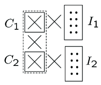
Proof: Fix $\delta\in(0,1)$ and consider, for simplicity, $n$ such that $\delta n$, $n$ are even. The graph $G_{n}$ is defined as follows. The nodes of $G_{n}$ are partitioned into four sets denoted $C_{1},C_{2},I_{1},I_{2}$, where $\left|{C_{1}}\right|=\left|{C_{2}}\right|=\delta n/2$, $\left|{I_{1}}\right|=\left|{I_{2}}\right|=(1-\delta)n/2$. The sets $C_{1},C_{2}$ are complete subgraphs and $I_{1},I_{2}$ are independent sets (see Figure 1). The pairs of sets $(I_{1},C_{1})$, $(C_{1},C_{2})$, $(C_{2},I_{2})$ are connected with complete bipartite graphs (i.e., every node in $I_{1}$ is connected to every node in $C_{1}$ and similarly for the other pairs). The resulting graph contains a clique $C=C_{1}\cup C_{2}$ of size $\delta n$.

We proceed by case analysis. Let $v_{\min}$ denote the node with the globally minimal ID in $G_{n}$, as drawn by the shingle algorithm.
Case 1: $v_{\min}\in C_{1}\cup C_{2}$. W.l.o.g assume that $v_{\min}\in C_{1}$. Then $v_{\min}$’s candidate set contains exactly $C_{1}\cup C_{2}\cup I_{1}$, a set whose density is

$$\frac{\binom{\left|{C_{1}}\right|+\left|{C_{2}}\right|}{2}+\left|{I_{1}}\right|\cdot\left|{C_{1}}\right|}{\binom{\left|{C_{1}}\right|+\left|{C_{2}}\right|+\left|{I_{1}}\right|}{2}}=\frac{\binom{\delta n}{2}+\delta(1-\delta)n^{2}/4}{\binom{(1+\delta)n/2}{2}}=\frac{2\delta}{1+\delta}~{},$$

and for $\epsilon<\frac{1-\delta}{1+\delta}$ the density is less than $1-\epsilon$. Clearly in this case all other candidates are subsets of $I_{1}\cup I_{2}$ and thus have density $0$.
Case 2: $v_{\min}\in I_{1}\cup I_{2}$. W.l.o.g assume that $v_{\min}\in I_{1}$. Then $v_{\min}$’s candidate set is exactly $C_{1}\cup\{v_{\min}\}$ and thus has size $\delta n/2+1$ which is asymptotically smaller than $(1-\epsilon)\delta n$ for any constant $\epsilon<1/2$.
Finally, consider the other candidate sets in this case. Clearly all nodes in $C_{2}$ belong to the same candidate set. Let $A$ denote the set of vertices from $I_{1}\cup I_{2}$ belonging to $C_{2}$’s candidate set. If $\left|{A}\right|<\delta n/4$ then the candidate set size is $\left|{C_{2}}\right|+\left|{A}\right|<3\delta n/4$ which is less than $(1-\epsilon)\delta n$ for all $\epsilon\leq 1/4$. If $\left|{A}\right|\geq\delta n/4$ then the candidate set density is at most

$$\frac{\binom{\left|{C_{2}}\right|}{2}+\left|{C_{2}}\right|\cdot\left|{A}\right|}{\binom{\left|{C_{2}}\right|+\left|{A}\right|}{2}}\leq 1-\frac{1-4/\delta n}{3\cdot(3-4/\delta n)}$$

which is asymptotically less than $1-\epsilon$ for any $\epsilon$ smaller than $1/9$. The remaining candidate sets are subsets of $I_{1}\cup I_{2}$ and thus have density $0$. $\square$

Summary. The simple approaches demonstrate the basic difficulty of the distributed $\epsilon$-near clique problem: looking to distance 1 is not sufficient, but looking to distance 2 is too costly. The algorithm presented next finds a middle ground using sampling.

4 Algorithm

Below we present the algorithm for finding dense subgraphs. Analysis is presented in Section 5.

The basic idea.

Let $V^{\prime}\subseteq V$ be a set of nodes. Define $K(V^{\prime})$ to be the set of all nodes which are adjacent to all other nodes in $V^{\prime}$, i.e., $K(V^{\prime})\stackrel{{\scriptstyle\rm def}}{{=}}\left\{v\;:\;\Gamma(v)\supseteq V^{\prime}\setminus\left\{v\right\}\right\}$. Further define $T(V^{\prime})$ to be the set of nodes in $K(V^{\prime})$ that are adjacent to all nodes in $K(V^{\prime})$, i.e., $T(V^{\prime})\stackrel{{\scriptstyle\rm def}}{{=}}\left\{v\in K(V^{\prime})\;:\;\Gamma(v)\supseteq K(V^{\prime})\setminus\left\{v\right\}\right\}$. Our starting point is the following key observation (essentially made in [10]). If $D$ is a clique, then $D\subseteq K(D)$, and also, by definition, $D\subseteq T(D)$. Furthermore, $T(D)$ is a clique since each $v\in T(D)$ is adjacent to all vertices in $K(D)$ and in particular those in $T(D)$.

The algorithm finds a set which is roughly $T(D)$, where $D$ is the existing near-clique, by random sampling. Suppose that we are somehow given a random sample $X$ of $D$. Consider $K(X)$: it is possible that $K(X)\not\subseteq K(D)$, because $K(X)$ is the set of nodes that are adjacent to all nodes in $X$, but not necessarily to all nodes in $D$. We therefore relax the definitions of $K(X)$ and $T(X)$ to approximate ones $K_{\epsilon}(X)$ and $T_{\epsilon}(X)$. Finally, we overcome the difficulty of inability to sample $D$ directly (because $D$ is unknown), by taking a random sample $S$ of $V$, trying all its subsets $X\subseteq S$ ($|S|$ is polynomial in $1/\epsilon$), and outputting the maximal $T(X)$ found.

Description and implementation details.

We now present the algorithm in detail. We shall use the following notation. Let $X\subseteq V$ be a set of nodes, and let $0\leq\epsilon\leq 1$. We denote by $K_{\epsilon}(X)$ the set of nodes which are neighbors of all but an $\epsilon$-fraction of the nodes in $X$, i.e.,

$$K_{\epsilon}(X)~{}\stackrel{{\scriptstyle\rm def}}{{=}}~{}\left\{v\in V\;:\;|\Gamma(v)\cap X|\geq(1-\epsilon)|X|\right\}~{}.$$ (1)

Using the notion of $K_{\epsilon}$, we also define

$$T_{\epsilon}(X)~{}\stackrel{{\scriptstyle\rm def}}{{=}}~{}K_{\epsilon}(K_{2\epsilon^{2}}(X))\,\cap\,K_{2\epsilon^{2}}(X)~{}.$$ (2)

  Algorithm $\mathsf{DistNearClique}$

 

Input

: Graph $G=(V,E)$, $\epsilon>0$, $p\in(0,1)$.

Output

: A label $\textsf{label}_{v}\in V\cup\left\{\bot\right\}$ at each node $v$, such that $u$ and $v$ are in the same near clique iff $\textsf{label}_{v}=\textsf{label}_{u}\neq\bot$.

 

Sampling stage.

Each node joins a set $S$ with probability $p$ (i.i.d). Let $G[S]$ denote the subgraph of $G$ induced by $S$.

Exploration stage:

Finding near-clique “candidates”.

• Construct a rooted spanning tree for each connected component of $G[S]$. By the end of this step, each node $v\in S$ has a variable $\textsf{parent}(v)$ that points to one of its neighbors (for the root, $\textsf{parent}(v)=\texttt{NULL}$).

• Each node in $S$ finds the identity of all nodes in its connected component and stores them in a variable $\textsf{Comp}(v)$.

• Each node $v\in S$ sends $\textsf{Comp}(v)$ to all its neighbors $\Gamma(v)$. A node $u\in\Gamma(S)$ may receive at this step messages from several nodes, that may or may not be in different components of $S$. Each node $u\in\Gamma(S)$ sets a parent pointer $\textsf{parent}_{S_{i}}(u)$ for each connected component $S_{i}$ of $G[S]$ that $u$ is adjacent to (choosing arbitrarily between its neighbors from the same $S_{i}$).

• Let $u\in\Gamma(S)$. Let $S_{1},\ldots,S_{\ell}$ be the different connected components which are adjacent to $u$. For each $S_{i}$ where $1\leq i\leq\ell$, the following procedure is executed.

  • For all subsets $X\subseteq S_{i}$, $u$ determines (using the information received in Step 3) if $u\in K_{2\epsilon^{2}}(X)$.

  • $u$ sends the results of the computations ($2^{|S_{i}|}$ bits) to all its neighbors, including $\textsf{parent}_{S_{i}}(u)$.

  • This information is sent up to the root of $S_{i}$, summing the counts for each $X$ along the way, so that the root of $S_{i}$ knows the value of $|K_{2\epsilon^{2}}(X)|$ for each $X\subseteq S_{i}$.

  • The root sends the value of $|K_{2\epsilon^{2}}(X)|$ down back to all nodes in $\Gamma(S_{i})$.

  • Each node $v\in K_{2\epsilon^{2}}(X)$ sends $|K_{2\epsilon^{2}}(X)|$ to all its neighbors, for each $X\subseteq S_{i}$.

  • Each node $u\in\Gamma(S_{i})$ finds whether $u\in K_{\epsilon}(K_{2\epsilon^{2}}(X))$ for each $X\subseteq S_{i}$, and thus determines whether $u\in T_{\epsilon}(X)$ for each $X$.

Decision stage:

Conflict resolution.

• For each connected component $S_{i}$, the size of $T_{\epsilon}(X)$ is computed for each $X\subseteq S_{i}$ similarly to Steps 4b–4c of the exploration stage. Let $X(S_{i})$ be the subset that maximizes $|T_{\epsilon}(X)|$ over all $X\subseteq S_{i}$.

• The root of each component $S_{i}$ sends $|T_{\epsilon}(X(S_{i}))|$ out to all nodes in $\Gamma(S_{i})$.

• After receiving $|T_{\epsilon}(X(S_{i}))|$ for all relevant connected components, each node sends an “acknowledge” message to the component reporting the largest $|T_{\epsilon}(X(S_{i}))|$, breaking ties in favor of the largest root ID, and an “abort” message to all other components.

• If no node in $\Gamma(S_{i})$ sent an “abort” message to $S_{i}$, the root sends back the result to all nodes in $T_{\epsilon}(X(S_{i}))$ (this is done by sending $X(S_{i})$). The label of a node in $T_{\epsilon}(X(S_{i}))$ is the root ID of $S_{i}$, and $\bot$ otherwise.

 

The algorithm works in stages as follows. In the sampling stage, a random sample of nodes $S$ is selected; the exploration stage generates near-clique candidates by considering $T_{\epsilon}(X)$ for all $X\subseteq S_{i}$ s.t. $S_{i}$ is a connected component of the induced subgraph $G[S]$; and the decision stage resolves conflicts between intersecting candidates. Pseudo-code for Algorithm $\mathsf{DistNearClique}$ is presented above. A detailed explanation of the distributed implementation of Algorithm $\mathsf{DistNearClique}$ follows.

The sampling stage is trivial: each node locally flips a biased coin, so that the node enters $S$ with probability $p$ ($p$ is a parameter to be fixed later). This step is completely local, and by its end, each node knows whether it is a member of $S$ or not.

The exploration stage is the heart of our algorithm. To facilitate it, we first construct a spanning tree for each connected components of $G[S]$ (Step 1 of the exploration stage). This construction is implemented by constructing a BFS spanning tree of each connected component $S_{i}$, rooted at the node with the smallest ID in $S_{i}$. This is a standard distributed procedure (see, e.g., [20]), but here only the nodes in $S$ take part, and all other nodes are non-existent for the purpose of this protocol.

In Step 2 of the exploration stage, all nodes send their IDs to the root. Once the root has all IDs, it sends them back down the tree.

In Step 3 of the exploration stage, each node in $S_{i}$ sends the identity of all nodes in $S_{i}$ to all its neighbors. In addition, we effectively add to each spanning tree all adjacent nodes. This is important so that we avoid over-counting later. Note that a node of $S$ is member of a single tree (the tree of its connected component), but a node in $V\setminus S$ may have more than one parent pointer: it has exactly one pointer for each component it is adjacent to.

Step 4 of the exploration stage determines for each node its membership in $T_{\epsilon}(X)$ for each subset $X$ of each connected component. Consider a node $u\in\Gamma(S_{i})$. After Step 3, $u$ knows the IDs of all members of $S_{i}$, so it can locally enumerate all $2^{|S_{i}|}$ subsets $X\subseteq S_{i}$, and furthermore, $u$ can determine whether $u\in K_{2\epsilon^{2}}(X)$ for each such subset $X$. Thus, each such node $u$ locally computes $2^{|S_{i}|}$ bits: one for each possible subset $X\subseteq S_{i}$. We assume that the coordinates of the resulting vector are ordered in a well known way (say, lexicographically). These vectors are sent by each node $u\in\Gamma(S_{i})$ to all its neighbors, and in particular to its parent in $S_{i}$. This is done by $u$ for each $S_{i}$ it is adjacent to. Step 4c is implemented using standard convergecast on the tree spanning $S_{i}$: the vectors are summed coordinate-wise and sent up the tree, so that when the information reaches the root of $S_{i}$, it knows the size of $K_{2\epsilon^{2}}(X)$ for each $X\subseteq S_{i}$. Finally, using the size of $K_{2\epsilon^{2}}(X)$, and knowing which of its neighbors is in $K_{2\epsilon^{2}}(X)$, each node $u$ can determine whether $u\in K_{\epsilon}(K_{2\epsilon^{2}}(X))$, and thus decide whether it is in $T_{\epsilon}(X)$ for each of the possible subsets $X$.

When the decision stage of Algorithm $\mathsf{DistNearClique}$ starts, each connected component $S_{i}$ of $G[S]$ has a “candidate” near-clique and we need to choose the largest $T_{\epsilon}(X)$ over all $X$’s. The difficulty is that there may be more than one set that qualifies as a near-clique, and these sets may overlap. Just outputting the union of these sets may be wrong because in general, the union of $\epsilon$-near clique need not be an $\epsilon$-near clique. The decision stage resolves this difficulty by allowing each node to “vote” only for the largest subset it is a member of. This vote is implemented by killing all other subsets using ‘abort’ messages, which is routed to the root of the spanning tree constructed in the exploration stage. This ensures that from each collection of overlapping sets, the largest one survives. Some small node sets may also have non-$\bot$ output: they can be disqualified if a lower bound on the size of the dense subgraph is known.

4.1 Wrappers

To conclude the description of the algorithm, we explain how to obtain a deterministic upper bound on the running time, and how to decrease error probability.

$\bullet$ Bounding the running time. As we argue in Section 5.1, the time complexity of the algorithm can be bounded with some constant probability. If a deterministic bound on the running time is desired, one can add a counter at each node, and abort the algorithm if the running time exceeds the specified time limit.

$\bullet$ Boosting the success probability. The way to decrease the failure probability is not simply running the algorithm multiple times. Rather, only the sampling and exploration stages are run several times independently, and then apply a single decision stage to select the output. More specifically, say we want to achieve success probability of at least $1-q$ for some given $q>0$. Let $\lambda\stackrel{{\scriptstyle\rm def}}{{=}}\log_{1-r}q$. To get failure probability at most $q$, we run $\lambda$ independent versions of the sampling and exploration stages (in any interleaving order). These $\lambda$ versions are run with a deterministic time bound as explained above. When all versions terminate, a single decision stage is run, and in Step 3 of the decision stage, nodes consider candidates from all $\lambda$ versions, and choose (by sending “acknowledge”) only the largest of these candidates. This boosting wrapper increases the running time by a factor of $\lambda$: the sampling and exploration stages are run $\lambda$ times, and the decision stage is slower by a factor of $\lambda$ due to congestion on the links.

5 Analysis

In this section we sketch the analysis of Algorithm $\mathsf{DistNearClique}$ presented in Section 4. Full details (i.e., most proofs) are presented in the appendix.

5.1 Complexity

We first state the time complexity in terms of the sample size, and then bound the sample size.

Lemma 5.1

Let $S$ be the set of nodes sampled in the sampling stage of Algorithm $\mathsf{DistNearClique}$. Then the round complexity of the algorithm is at most $O\left(2^{\left|{S}\right|}\right)$.

Lemma 5.2

$\Pr[\left|{S}\right|\leq 2pn]\geq 1-e^{-\frac{pn}{3}}$.

5.2 Correctness

In this section we prove that Algorithm $\mathsf{DistNearClique}$ finds a large near-clique. We note that while the algorithm appears similar to the $\rho$-clique algorithm in [10], the analysis of Algorithm $\mathsf{DistNearClique}$ is different. We need to account for the fact that the input contains a near-clique (rather than a clique), and we need to establish certain locality properties to show feasibility of a distributed implementation.

For the remainder of this section, fix $G=(V,E)$, $\epsilon>0$, and $\delta>0$. Let $\left|{V}\right|=n$. Assume that $D\subseteq V$ is an $\epsilon^{3}$-near clique satisfying $\left|{D}\right|\geq\delta n$. Recall that $G[S]$ denotes the subgraph of $G$ induced by $S$. In addition, assume that $\epsilon<\frac{1}{{3}}$ (larger values are meaningless, see parameters of Theorem 5.7).

Let $D^{\prime}$ denote the set of nodes output by Algorithm $\mathsf{DistNearClique}$. Clearly, $D^{\prime}=T_{\epsilon}(X)$ for some $X$. We first show that every $T_{\epsilon}(X)$ is $\frac{n}{t}\epsilon$-near clique where $t=|T_{\epsilon}(X)|$. In the decision stage, the algorithm selects the largest $T_{\epsilon}(X)$. In Lemma 5.6, we prove our main technical result, namely that with constant probability, there exists a subset $X^{*}\subseteq S_{i}$ with $\left|{T_{\epsilon}(X^{*})}\right|\geq(1-(\epsilon))\left|{D}\right|$.

All large $T_{\epsilon}(X)$ are near-cliques.

The following lemma proves that any $T_{\epsilon}(X)$ is a near-clique with a parameter relating to its size.

Lemma 5.3

Let $X\subseteq V$, and denote $t=\left|{T_{\epsilon}(X)}\right|$. Then $T_{\epsilon}(X)$ is $\frac{n\epsilon}{t}$-near clique.

Existence of a large $T_{\epsilon}(X)$.

We prove the existence of a connected set $X^{*}\subseteq S$ such that $T_{\epsilon}(X^{*})$ is large.

First, let $C$ denote the set of all nodes in the $\epsilon^{3}$-near clique $D$ that are also adjacent to all but $\epsilon^{2}$ fraction of $D$. Formally: $\displaystyle C\stackrel{{\scriptstyle\rm def}}{{=}}K_{\epsilon^{2}}(D)\cap D~{}\mbox{ where $D$ is $\epsilon^{3}$-near clique.}$ We use the following simple property.

Lemma 5.4

$\left|{C}\right|\geq(1-\epsilon)\left|{D}\right|-{1\over\epsilon^{2}}$.

Second, we structure the probability space defined by the sampling stage of Algorithm $\mathsf{DistNearClique}$ as follows. In the algorithm, each node flips a coin with probability $p$ of getting “heads” (i.e., entering $S$). We view this as a two-stage process, where each node flips two independent coins: ${\sf coin}_{1}$ with probability $p_{1}\stackrel{{\scriptstyle\rm def}}{{=}}p/2$ of getting “heads” and ${\sf coin}_{2}$ with probability $p_{2}\stackrel{{\scriptstyle\rm def}}{{=}}\frac{p-p_{1}}{1-p_{1}}>p/2$ of getting “heads.” A node enters $S$ iff at least one of its coins turned out to be “heads.” The idea is that the net result of the process is that each node enters $S$ independently with probability $p$, but this refinement allows us to define two subsets of $S$: let $S^{(1)}$ be the set of nodes for which ${\sf coin}_{1}$ is heads, and let $S^{(2)}$ be the set of nodes for which ${\sf coin}_{2}$ is heads.

Combining the notions, we define $X^{*}\stackrel{{\scriptstyle\rm def}}{{=}}S^{(1)}\cap C$, i.e., $X^{*}$ is a random variable representing the set of nodes from $C$ for which ${\sf coin}_{1}$ is heads. $X^{*}$ is effectively a sample of $C$ where each node is selected with probability $p/2$. We have the following.

Lemma 5.5

$X^{*}$ resides within a single connected component of $G[S]$ with probability at least $1-e^{-\Omega\left(\delta pn\right)}$.

We now arrive at our main lemma.

Lemma 5.6

With probability at least $1-\frac{1}{{\epsilon^{2}\delta}}e^{-\Omega\left(\epsilon^{4}\delta\cdot pn\right)}$ over the selection of $S$, there exists a connected component $S_{i}$ of $G[S]$ and a set $X^{*}\subseteq S_{i}$ s.t. $\left|{T_{\epsilon}(X^{*})}\right|\geq(1-\frac{13}{2}\epsilon)\left|{D}\right|-\epsilon^{-2}$.

Proof: Let $X^{*}$ be defined as above. It remains to show that $T_{\epsilon}(X^{*})$ is large. Intuitively, $X^{*}$ is a random sample of $C$, and since $C$ contains almost all of $D$, $X^{*}$ is also, in a sense, a sample of $D$. Thus $K_{2\epsilon^{2}}(X^{*})$ should be very close to $K_{(\cdot)}(C)$, $K_{(\cdot)}(D)$ for appropriately selected $(\cdot)$. This would complete the proof since $T_{\epsilon}(C)$ contains almost all of $C$ which, in turn, contains almost all of $D$. Formally, we say that $X^{*}$ is representative if the following hold.

• $\left|{K_{\epsilon^{2}}(D)\setminus K_{2\epsilon^{2}}(X^{*})}\right|<\epsilon\left|{C}\right|$.

• $\left|{K_{2\epsilon^{2}}(X^{*})\setminus K_{3\epsilon^{2}}(C)}\right|<\epsilon^{2}\left|{C}\right|$.

That is, if $K_{2\epsilon^{2}}(X^{*})$ is almost fully contained in $K_{\epsilon^{2}}(D)$ and almost fully contains $K_{3\epsilon^{2}}(C)$.

To complete the proof, we use two claims presented below. Claim 2 shows that if $X^{*}$ is representative, then $\left|{C\setminus T_{\epsilon}(X^{*})}\right|\leq\frac{11}{2}\epsilon\cdot\left|{C}\right|$. Claim 3 shows that $X^{*}$ is representative with probability $1-\frac{1}{{\epsilon^{2}\delta}}e^{-\Omega\left(\epsilon^{4}\delta pn\right)}$. Given these claims, the proof is completed as follows. By Lemma 5.5 and the claims, we have that $1-(e^{-\Omega(\delta pn)}-\frac{1}{{\epsilon^{2}\delta}}e^{-\Omega\left(\epsilon^{4}\delta pn\right)})$, we have that $X^{*}$ resides in a connected component of $G[S]$, and, using also Lemma 5.4 the proof is complete, because

$$\left|{T_{\epsilon}(X^{*})}\right|~{}\geq~{}\left(1-\frac{11}{2}\epsilon\right)\left|{C}\right|~{}\geq~{}\left(1-\frac{11}{2}\epsilon\right)\left((1-\epsilon)\left|{D}\right|-{1\over\epsilon^{2}}\right)~{}\geq~{}\left(1-\frac{13}{2}\epsilon\right)\left|{D}\right|-{1\over\epsilon^{2}}~{}.\quad\hfill\square$$

Claim 2

If $X^{*}$ is representative, then $\left|{C\setminus T_{\epsilon}(X^{*})}\right|\leq\frac{11}{2}\epsilon\cdot\left|{C}\right|$

Claim 3

$\Pr\left[X^{*}\mbox{ is representative}\right]\geq 1-\frac{1}{{\epsilon^{2}\delta}}\cdot e^{-\Omega\left(\epsilon^{4}\delta pn\right)}$.

5.3 Summary

We summarize with the following theorem, which is the detailed version of Theorem 2.1 (in Theorem 2.1, we set $p=\frac{1}{{n}}\cdot O\left(\frac{\log(\frac{1}{{\epsilon\delta}})}{\epsilon^{4}\delta}\right)$).

Theorem 5.7

Let $G=(V,E)$, $\left|{V}\right|=n$. Let $D\subseteq V$ be an $\epsilon^{3}$-near clique in $G$ of size $\left|{D}\right|\geq\delta n$. Then with probability at least $1-\frac{1}{\epsilon^{2}\delta}\cdot e^{-\Omega\left(\epsilon^{4}\delta\cdot pn\right)}$, Algorithm $\mathsf{DistNearClique}$, running on $G$ with parameters $\epsilon,p$, finds, in $O\left(2^{2pn}\right)$ communication rounds, a subgraph $D^{\prime}$ such that

• $D^{\prime}$ is $\left(\frac{1}{{(1-\frac{13}{2}\epsilon)}}\cdot\frac{\epsilon}{\delta}\right)$-near clique.

• $\left|{D^{\prime}}\right|\geq(1-\frac{13}{2}\epsilon)\left|{D}\right|-\epsilon^{-2}$.

Proof: By Lemmas 5.1 and 5.2, the probability that the round complexity exceeds $2^{O\left(2pn\right)}$ is bounded by $e^{-\frac{pn}{3}}$. By Lemma 5.3, whenever assertion (2) holds, assertion (1) holds as well. Assertion (2) holds by Lemma 5.6 with probability at least $1-\frac{1}{{\epsilon^{2}\delta}}e^{-\Omega\left(\epsilon^{4}\delta\cdot pn\right)}$. The theorem follows from the union bound. $\square$

It may also be interesting to analyze the computational complexity of the vertices running the algorithm. A simple analysis shows that except for step 4f of the exploration stage, the operation for each node can be implemented in ${\rm poly}(\left|{S}\right|)$ computational steps (on $\log n$ bit numbers) per communication round. In step 4f, however, the nodes need to “inspect” all their neighbors in order to determine whether they reside in $T_{\epsilon}(X)$. It is possible to reduce the complexity in this case by selecting a sample of the neighbors and estimating, rather than determining, membership in $T_{\epsilon}(X)$. Thus, the computational complexity can be reduced to ${\rm poly}(\left|{S}\right|)$ computational steps per round (for our purposes, $|S|\leq O(\log\log n)$). The analysis of this modification is omitted.

6 Discussion

On the impossibility of finding a globally maximal $\epsilon$-near clique.

Our algorithm (when successful) finds a disjoint collection of near-cliques such that at least one of them is large. We note that it is impossible for a distributed sub-diameter time algorithm to output just one (say, the largest) clique. To see that, consider a graph containing an $n/2$-vertex clique $A$ and an $n/4$-vertex clique $B$, connected by an $n/4$-long path $P$. The largest near-clique in this case is obviously $A$, and the vertices of $B$ should output $\bot$. However, if we delete all edges in $A$, the largest near-clique becomes $B$, i.e., its output must be non-$\bot$. Since no node in $B$ can distinguish between the two scenarios in less than $|P|=n/4$ communication rounds, impossibility follows.

Deriving distributed algorithms from property testers.

Our approach may raise hopes that other property testers, at least in the dense graph model, can be adapted into the distributing setting. Goldreich and Trevisan [11] prove that any property tester in the dense graph model has a canonical form where the first stage is selecting a uniform sample of appropriate size from the graph and the second is testing the graph induced by the sample for some (possibly other) property. Thus, the following scheme may seem likely to be useful:
1. Select a uniform sample by having all nodes flip a biased coin.
2. Find the graph induced between sampled nodes. This graph has very small (possibly constant) size.
3. Use some (possibly inefficient) distributed algorithm to test it for the required property.
In the distributed setting, however, sometime even testing a property for a very small graph would be impossible due to connectivity issues. As demonstrated above, there exist properties that are testable in the centralized setting and do not admit an efficient round-complexity distributed algorithm. The general method above, therefore, can only be applied in a “black-box” manner for some testers.

Specifically, the $\rho$-clique tester presented in [10] does not comply with the above requirements (specifically, as we mentioned, the $\rho$-clique problem is unsolvable in small round-complexity). It can, however, be converted into a near-clique finder, in the sense defined in this work, using similar ideas and with worse parameters.

APPENDIX: Additional Proofs

Proof of Lemma 5.1:  The sampling stage requires no communication. Consider now the exploration stage. The BFS tree construction of Step 1 uses messages of $O(\log n)$ bits (each message contains an ID and a distance counter), and its running time is proportional to the diameter of the component, which is trivially bounded by $|S|$. The number of rounds to execute Step 2 is proportional to the number of IDs plus the height of the tree, due to the pipelining of messages: the number of hops each ID needs to travel is at most twice the tree height, and a message needs to wait at most once for each other ID. It follows that the total time required for this step in $O(|S|)$ rounds. Step 3 takes at most $\max_{i}\left\{|S_{i}|\right\}\leq|S|$ rounds. Step 4a requires no communication. Step 4b requires a node $u$ to send $0$ or $1$ for each subset of each component of $S$ it is adjacent to. Since there may be at most $2^{|S|}$ such subsets (over all components), this step takes at most $O(2^{|S|})$ rounds. In Step 4c, each entry of the vector may be a number between $0$ and $n$, and hence the total number of bits in a vector is at most $2^{|S|}\log n$; using pipelining once again, we can therefore bound the number of rounds required to execute Step 4c by $O(2^{|S|}+|S|)=O(2^{|S|})$. Similarly for Steps 4d–4e. Step 4f is local; In the decision stage, Step 1 takes, again, at most $O(2^{|S|})$ rounds. The remaining steps take at most $O(\max_{i}\left|{S_{i}}\right|)\leq O(\left|{S}\right|)$ rounds. Thus the total round complexity of Algorithm $\mathsf{DistNearClique}$ is at most $O\left(2^{\left|{S}\right|}\right)$. $\square$

Proof of Lemma 5.2:  Follows from the Chernoff Bound, since in the sampling stage, each of the $n$ nodes join $S$ independently with probability $p$. $\square$

Proof of Lemma 5.3:  By counting. Recall that each undirected edge is viewed and counted as two anti-symmetrical directed edges. Define $Y=K_{2\epsilon^{2}}(X)$. Consider a node $v\in T_{\epsilon}(X)$. By definition of $T_{\epsilon}(X)$, $v\in K_{\epsilon}(Y)$, i.e.,

$$\left|{\Gamma(v)\cap Y}\right|~{}\geq~{}(1-\epsilon)\left|{Y}\right|~{}.$$ (3)

Since $T_{\epsilon}(X)\subseteq Y$, we have $\left|{\Gamma(v)\cap T_{\epsilon}(X)}\right|~{}\geq~{}\left|{\Gamma(v)\cap Y}\right|~{}\geq~{}t-\epsilon\left|{Y}\right|$ by Eq. (3). Since $|Y|\leq n$, we can conclude that $\left|{\Gamma(v)\cap T_{\epsilon}(X)}\right|\geq(1-\frac{n}{t}\epsilon)t$. It follows that the total number of (directed) edges in $T_{\epsilon}(X)$ is at least $(1-\frac{n}{t}\epsilon)t(t-1)$, as required. $\square$ $\square$

Proof of Lemma 5.4:  Denote $c\stackrel{{\scriptstyle\rm def}}{{=}}|C|$ and $d\stackrel{{\scriptstyle\rm def}}{{=}}|D|$. Since $D$ is an $(1-\epsilon^{3})$-near clique in $G$, we have that

$$|E\cap(D\times D)|~{}\geq~{}(1-\epsilon^{3})d(d-1)~{}\geq~{}(1-\epsilon^{3})d^{2}-d~{}.$$ (4)

By definition of $C$, if $v\in D\setminus C$, then

$$|E\cap(\left\{v\right\}\times D)|<(1-\epsilon^{2})d~{}.$$ (5)

Now, if we assume that $c<(1-\epsilon-{1\over\epsilon^{2}d})d$, we arrive at a contradiction to Eq. (4), since

$$|E\cap(D\times D)| = |E\cap(C\times D)|+|E\cap((D\setminus C)\times D)|$$

$$\leq c\cdot d+(d-c)(1-\epsilon^{2})d~{}~{}~{}~{}~{}~{}~{}~{}~{}~{}~{}~{}~{}~{}~{}~{}~{}~{}~{}~{}~{}~{}~{}~{}~{}~{}~{}~{}~{}~{}~{}\mbox{by Eq.~{}(\ref{eq:d+1})}$$

$$= (1-\epsilon^{2})\cdot d^{2}+\epsilon^{2}\cdot c\cdot d$$

$$< (1-\epsilon^{2})\cdot d^{2}+\epsilon^{2}\left((1-\epsilon)d-{1\over\epsilon^{2}}\right)d~{}~{}~{}~{}~{}~{}~{}~{}~{}~{}~{}~{}~{}~{}~{}\mbox{if $c<(1-\epsilon)d-{1\over\epsilon^{2}}$}$$

$$\leq (1-\epsilon^{3})d^{2}-d~{}.$$

$\square$

Proof of Lemma 5.5:  We show that a stronger property holds with that probability: namely, that the distance in $S$ between any two nodes of $X^{*}$ is at most $2$. By definition, $X^{*}\subseteq C$, i.e., $X^{*}\subseteq K_{\epsilon^{2}}(D)$. It follows from the pigeonhole principle that every two nodes $u,v\in X^{*}$ have at least $(1-2\epsilon^{2})\left|{D}\right|$ common neighbors. The probability that none of these common neighbors is in $S^{(2)}$ (i.e., that none of them has outcome heads for ${\sf coin}_{2}$) is therefore at most $(1-p_{2})^{(1-2\epsilon^{2})\left|{D}\right|}\leq e^{-(1-2\epsilon^{2})p_{2}\left|{D}\right|}\leq e^{-\frac{7}{18}p\left|{D}\right|}$ for $\epsilon\leq 1/3$, and because $p_{2}>p/2$ by definition. We now apply the union bound to obtain that $\Pr\left[\mbox{diameter}(X^{*})>2\right]\leq\left|{X^{*}}\right|\cdot e^{-\frac{7}{18}p\left|{D}\right|}$. Since $X^{*}$ is a random sample of $C$, it follows that ${\mathbb{E}}[\left|{X^{*}}\right|]=p_{2}\cdot\left|{C}\right|\leq p\delta n$. Using a Chernoff bound, we obtain that $\Pr[\left|{X^{*}}\right|>2p\delta n]\leq e^{-\Omega\left(\delta pn\right)}$. Therefore, by the union bound

$$\Pr\left[\mbox{diameter}(X^{*})>2\right] \leq \Pr\left[\mbox{diameter}(X^{*})>2~{}|~{}\left|{X^{*}}\right|\leq 2p\delta n\right]+\Pr\left[\left|{X^{*}}\right|>2p\delta n\right]$$

$$\leq 2\delta pn\cdot e^{-\Omega\left(\delta pn\right)}+e^{-\Omega\left(\delta pn\right)}\leq e^{-\Omega\left(\delta pn\right)}~{}.\qquad\qquad\qquad\qquad\qquad\hfill\square$$

Proof of Claim 2:  By definition,

$$\left|{C\setminus T_{\epsilon}(X^{*})}\right|~{}\leq~{}\left|{C\setminus K_{2\epsilon^{2}}(X^{*})}\right|+\left|{C\setminus K_{\epsilon}(K_{2\epsilon^{2}}(X^{*}))}\right|~{}.$$ (6)

We bound each term in Eq. (6) in turn.

First, note that $\left|{K_{\epsilon^{2}}(D)\setminus K_{2\epsilon^{2}}(X^{*})}\right|<\epsilon\left|{C}\right|$, because $X^{*}$ is representative. It follows that

$$\left|{C\setminus K_{2\epsilon^{2}}(X^{*})}\right|<\epsilon\left|{C}\right|~{},$$ (7)

because $C\subseteq K_{\epsilon^{2}}(D)$. Note that Eq. (7) also implies for $\epsilon\leq 1/3$ that

$$\left|{K_{2\epsilon^{2}}(X^{*})}\right|~{}\geq~{}(1-\epsilon)\left|{C}\right|~{}\geq~{}\frac{2\left|{C}\right|}{3}~{}.$$ (8)

We now turn to the second term of Eq. (6). $X^{*}$ is representative, and therefore $\left|{K_{2\epsilon^{2}}(X^{*})\setminus K_{3\epsilon^{2}}(C)}\right|<\epsilon^{2}\left|{C}\right|$, i.e., all but $\epsilon^{2}\left|{C}\right|$ vertices of $K_{2\epsilon^{2}}(X^{*})$ are neighbors of at least $(1-3\epsilon^{2})|C|$ nodes of $C$. Let $Y=C\setminus K_{\epsilon}(K_{2\epsilon^{2}}(X^{*}))$, $y=\left|{Y}\right|$, and $z=\left|{K_{2\epsilon^{2}}(X^{*})}\right|$. Counting the number of edges between $C$ and $K_{2\epsilon^{2}}(X^{*})$ we conclude that $y\cdot(1-\epsilon)z+(\left|{C}\right|-y)\cdot z\geq\left(z-\epsilon^{2}\left|{C}\right|\right)(1-3\epsilon^{2})\left|{C}\right|$, and plugging in Eq. (8) we obtain

$$y\cdot(1-\epsilon)z+(\left|{C}\right|-y)\cdot z\geq z\cdot(1-\frac{3\epsilon^{2}}{2})(1-3\epsilon^{2})\left|{C}\right|\geq(1-\frac{9\epsilon^{2}}{2})\cdot z\left|{C}\right|~{}.$$

Rearranging, we have $y\leq\frac{9\epsilon}{2}\cdot\left|{C}\right|$, and the claim follows. $\square$

Proof of Claim 3:  Since ${\mathbb{E}}[\left|{X^{*}\!}\right|]=p_{1}\left|{C}\right|$, and since membership in $X^{*}$ is determined independently for each node, we can apply the Chernoff Bound to obtain that

$$\Pr\left[\Big{|}\left|{X^{*}\!}\right|-{\mathbb{E}}\big{[}\left|{X^{*}\!}\right|\big{]}\Big{|}>\frac{\epsilon^{2}}{4}{\mathbb{E}}\big{[}\left|{X^{*}\!}\right|\big{]}\right]~{}<~{}2\exp\left({-\frac{1}{{3}}\left(\frac{\epsilon^{2}}{4}\right)^{2}{\mathbb{E}}\big{[}\left|{X^{*}\!}\right|\big{]}}\right)~{}\leq~{}2\exp\left(-{\epsilon^{4}p_{1}\left|{C}\right|\over 48}\right).$$

Assume that $\Big{|}{\left|{X^{*}}\right|-{\mathbb{E}}\big{[}\left|{X^{*}\!}\right|\big{]}}\Big{|}\leq\frac{\epsilon^{2}}{4}{\mathbb{E}}\big{[}\left|{X^{*}\!}\right|\big{]}$, and let us consider the definition of a representative set.

For item 1, let $v\in K_{\epsilon^{2}}(D)$. Then $\left|{\Gamma(v)\cap C}\right|\geq\left|{C}\right|-\epsilon^{2}\left|{D}\right|\geq\left|{C}\right|-\frac{\epsilon^{2}}{1-\epsilon}\left|{C}\right|\geq(1-\frac{3}{2}\epsilon^{2})\left|{C}\right|$. Since $\Gamma(v)\cap X^{*}$ is a random sample of $\Gamma(v)\cap C$, where each member is chosen with probability $p_{1}$, we have that ${\mathbb{E}}\left[\left|{\Gamma(v)\cap X^{*}}\right|\right]=p_{1}\cdot\left|{\Gamma(v)\cap C}\right|\geq(1-\frac{3}{2}\epsilon^{2})p_{1}\left|{C}\right|=(1-\frac{3}{2}\epsilon^{2}){\mathbb{E}}[\left|{X^{*}}\right|]$. Denote $Y_{v}=\left|{\Gamma(v)\cap X^{*}}\right|$. Then

$$\Pr[v\not\in K_{2\epsilon^{2}}(X^{*})] = \Pr[Y_{v}<(1-2\epsilon^{2})\left|{X^{*}\!}\right|]~{}\leq~{}\Pr\Big{[}Y_{v}<(1-2\epsilon^{2})(1+\frac{\epsilon^{2}}{4}){\mathbb{E}}[\left|{X^{*}\!}\right|]\Big{]}$$

$$\leq \Pr\Big{[}Y_{v}-{\mathbb{E}}[Y_{v}]<(1-2\epsilon^{2})(1+\frac{\epsilon^{2}}{4}){\mathbb{E}}[\left|{X^{*}\!}\right|]-(1-\epsilon^{2}){\mathbb{E}}[\left|{X^{*}\!}\right|]\Big{]}$$

$$\leq \Pr[Y_{v}-{\mathbb{E}}[Y_{v}]<-\frac{\epsilon^{2}}{4}{\mathbb{E}}[\left|{X^{*}\!}\right|]]$$

$$< \exp\left(-\frac{1}{{2}}\left(\frac{\frac{\epsilon^{2}}{4}{\mathbb{E}}[\left|{X^{*}\!}\right|]}{{\mathbb{E}}[Y_{v}]}\right)^{2}{\mathbb{E}}[Y_{v}]\right)$$

$$\leq \exp\left(-{\epsilon^{4}\over 32}{\mathbb{E}}[\left|{X^{*}\!}\right|]\right)~{}\leq~{}\exp\left(-{\epsilon^{4}\over 32}\cdot p_{1}\left|{C}\right|\right),$$

and therefore ${\mathbb{E}}[\left|{K_{\epsilon^{2}}(C)\setminus K_{2\epsilon^{2}}(X^{*})}\right|]<\exp\left(-{\epsilon^{4}\over 32}\cdot p_{1}\left|{C}\right|\right)\cdot n$. Using Markov’s Inequality we obtain

$$\Pr\Big{[}\left|{K_{\epsilon^{2}}(C)\setminus K_{2\epsilon^{2}}(X^{*})}\right|\geq\epsilon\left|{C}\right|\Big{]}~{}\leq~{}\frac{n}{\epsilon\left|{C}\right|}\cdot e^{-{\epsilon^{4}}\cdot p_{1}\left|{C}\right|/32}.$$

A similar argument applies to item 2. Consider a node $v\not\in K_{3\epsilon^{2}}(C)$ . Denote $Y_{v}=\left|{\Gamma(v)\cap X^{*}}\right|$. Then ${\mathbb{E}}[Y_{v}]<(1-3\epsilon^{2}){\mathbb{E}}[\left|{X^{*}\!}\right|]$, and therefore

$$\Pr[v\in K_{2\epsilon^{2}}(X^{*})] = \Pr[Y_{v}\geq(1-2\epsilon^{2})\left|{X^{*}\!}\right|]~{}\leq~{}\Pr\Big{[}Y_{v}\geq(1-2\epsilon^{2})(1-\frac{\epsilon^{2}}{4}){\mathbb{E}}[\left|{X^{*}\!}\right|]\Big{]}$$

$$\leq \Pr\Big{[}Y_{v}-{\mathbb{E}}[Y_{v}]\geq(1-2\epsilon^{2})(1-\frac{\epsilon^{2}}{4}){\mathbb{E}}[\left|{X^{*}\!}\right|]-(1-3\epsilon^{2}){\mathbb{E}}[\left|{X^{*}\!}\right|]\Big{]}$$

$$\leq \Pr\Big{[}Y_{v}-{\mathbb{E}}[Y_{v}]\geq\frac{3\epsilon^{2}}{4}{\mathbb{E}}[\left|{X^{*}\!}\right|]\Big{]}$$

$$< \exp\left(-\frac{1}{{3}}\left(\frac{\frac{3\epsilon^{2}}{4}{\mathbb{E}}[\left|{X^{*}\!}\right|]}{{\mathbb{E}}[Y_{v}]}\right)^{2}{\mathbb{E}}[Y_{v}]\right)$$

$$\leq \exp\left(-\frac{3\epsilon^{4}}{16}\cdot{\mathbb{E}}[\left|{X^{*}\!}\right|]\right)~{}\leq~{}\exp\left(-\frac{3\epsilon^{4}}{16}\cdot p_{1}\left|{C}\right|\right),$$

i.e., ${\mathbb{E}}[\left|{K_{2\epsilon^{2}}(X^{*})\setminus K_{3\epsilon^{2}}(C)}\right|]<\exp\left(-\frac{3}{16}\epsilon^{4}\cdot p_{1}\left|{C}\right|\right)\cdot n$, which implies, as above, that

$$\Pr\Big{[}\left|{K_{2\epsilon^{2}}(X^{*})\setminus K_{3\epsilon^{2}}(C)}\right|\geq\epsilon^{2}\left|{C}\right|\Big{]}~{}\leq~{}\frac{n}{\epsilon^{2}\left|{C}\right|}\cdot e^{-3\epsilon^{4}\cdot p_{1}\left|{C}\right|/16}.$$

Finally, we apply the Union Bound to that $X^{*}$ is representative with probability at least

$$1-\left(2e^{-\epsilon^{4}p_{1}\left|{C}\right|/48}+\frac{n}{\epsilon\left|{C}\right|}\cdot e^{-\epsilon^{4}\cdot p_{1}\left|{C}\right|/32}+\frac{n}{\epsilon^{2}\left|{C}\right|}\cdot e^{-{3}\epsilon^{4}\cdot p_{1}\left|{C}\right|/16}\right)~{}\geq~{}1-\frac{n}{\epsilon^{2}\left|{C}\right|}\cdot e^{-\Omega\left(\epsilon^{4}\cdot p\left|{C}\right|\right)}~{}.\quad\hfill\square$$

References

- [1] J. Abello, M. G. C. Resende, and S. Sudarsky. Massive quasi-clique detection. In LATIN, pages 598–612, 2002.
- [2] N. Alon, L. Babai, and A. Itai. A fast and simple randomized parallel algorithm for the maximal independent set problem. J. Algorithms, 7:567–583, 1986.
- [3] B. Awerbuch. Complexity of network synchronization. J. ACM, 32(4):804–823, Oct. 1985.
- [4] S. Basagni, M. Mastrogiovanni, A. Panconesi, and C. Petrioli. Localized protocols for ad hoc clustering and backbone formation: a performance comparison. IEEE Trans. Parallel and Dist. Systems., 17(4):292–306, April 2006.
- [5] S. Brin and L. Page. The anatomy of a large-scale hypertextual web search engine. Computer Networks and ISDN Systems, 30(1–7):107–117, 1998.
- [6] A. Z. Broder, S. C. Glassman, M. S. Manasse, and G. Zweig. Syntactic clustering of the web. Computer Networks and ISDN Systems, 29(8-13):1157 – 1166, 1997. Papers from the Sixth International World Wide Web Conference.
- [7] U. Feige, G. Kortsarz, and D. Peleg. The dense -subgraph problem. Algorithmica, 29(3):410–421, 2001.
- [8] U. Feige and M. Langberg. Approximation algorithms for maximization problems arising in graph partitioning. J. Algorithms, 41(2):174–211, Nov. 2001.
- [9] E. Fischer and I. Newman. Testing versus estimation of graph properties. In Proc. 37th Ann. ACM Symp. on Theory of Computing, pages 138–146, New York, NY, USA, 2005. ACM.
- [10] O. Goldreich, S. Goldwasser, and D. Ron. Property testing and its connection to learning and approximation. J. ACM, 45(4):653–750, 1998.
- [11] O. Goldreich and L. Trevisan. Three theorems regarding testing graph properties. Random Struct. Algorithms, 23(1):23–57, 2003. Preliminary version in FOCS ’01.
- [12] R. Gupta and J. Walrand. Approximating maximal cliques in ad-hoc networks”. In Proc. IEEE Int. Symp. on Personal, Indoor and Mobile Radio Communications, pages 365–369, Barcelona, Sept. 2004.
- [13] J. Håstad. Clique is hard to approximate within . Acta Mathematica, 182(1):105–142, 1999.
- [14] R. Kumar, J. Novak, P. Raghavan, and A. Tomkins. On the bursty evolution of blogspace. World Wide Web, 8(2):159–178, 2005.
- [15] R. Lempel and S. Moran. SALSA: the stochastic approach for link-structure analysis. ACM Trans. Inf. Syst., 19(2):131–160, 2001.
- [16] M. Luby. A simple parallel algorithm for the maximal independent set problem. SIAM J. Comput., 15(4):1036–1053, Nov. 1986.
- [17] H. N. Nguyen and K. Onak. Constant-time approximation algorithms via local improvements. In FOCS, pages 327–336. IEEE Computer Society, 2008.
- [18] M. Parnas and D. Ron. Approximating the minimum vertex cover in sublinear time and a connection to distributed algorithms. Theoretical Comput. Sci., 381(1-3):183–196, 2007.
- [19] M. Parnas, D. Ron, and R. Rubinfeld. Tolerant property testing and distance approximation. J. Comp. and Syst. Sci., 72(6):1012–1042, 2006. Preliminary version in STOC ’05.
- [20] D. Peleg. Distributed Computing: A Locality-Sensitive Approach. Society for Industrial and Applied Mathematics, Philadelphia, PA, USA, 2000.
- [21] R. Rubinfeld and M. Sudan. Robust characterizations of polynomials with applications to program testing. SIAM J. Comput., 25(2):252–271, 1996.
- [22] M. Saks and C. Seshadhri. Parallel monotonicity reconstruction. In Proc. 19th Ann. ACM-SIAM Symp. on Discrete algorithms, pages 962–971, Philadelphia, PA, USA, 2008. SIAM.