The exact three-dimensional half-shell t-matrix for a sharply cut-off Coulomb potential in the screening limit

Abstract

The three-dimensional half-shell t-matrix for a sharply cut-off Coulomb potential is analytically derived together with its asymptotic form without reference to partial wave expansion. The numerical solutions of the three-dimensional Lippmann-Schwinger equation for increasing cut-off radii provide half-shell t-matrices which are in quite a good agreement with the asymptotic values.

I Introduction

This is a continuation of a previous article Gl09 where the exact analytical three-dimensional wave function for a sharply cut-off Coulomb potential has been derived together with the corresponding scattering amplitude (the on-shell t-matrix). In the screening limit that scattering amplitude converges to a sum of two terms. One is the expected pure Coulomb scattering amplitude multiplied with the standard renormalisation factor $(2pR)^{-2i\eta}$; the other one is new and includes angular dependent phases $e^{\pm 2ipRsin\frac{\theta}{2}}$, which oscillate without limit for infinite screening radius R. As has been conjectured in Taylor that second term would disappear after integration over some angular intervals in the sense of a distribution.

We are now interested in the screening limit of the corresponding half-shell t-matrix. The pure Coulomb force result for that object is well known Kok . Its derivation goes back to work by Guth . Especially its discontinuous property at the on-shell point is of interest. In Ford64 ; Ford66 this property has been discussed based on a sharply cut-off Coulomb potential and using a partial wave decomposition. Like in our previous paper we felt that a direct three-dimensional approach avoids possibly open questions in that treatment related to the correct summation of the infinite number of partial wave components. (See Ford64 ; Ford66 , where the difficulties are spoken out leading in fact to incomplete results). We therefore study the half-shell t-matrix now based on the exact three-dimensional wave function for a sharply cut-off Coulomb potential and investigate its screening limit. The details of derivation are given in Section II. Numerical solutions of the three-dimensional Lippmann-Schwinger equation for different cut-off radii are compared with the asymptotic values in Section III. We summarize and conclude in Section IV.

II The half-shell t-matrix

For a a sharply cut-off repulsive Coulomb potential (for instance for two protons)

$$V_{R}(r)=\Theta(R-r)\frac{e^{2}}{r}$$ (1)

the exact three-dimensional wave function inside the potential range is given by

$$\Psi_{R}^{(+)}=Ae^{i\vec{p}\cdot\vec{r}}F(-i\eta,1,i(pr-\vec{p}\cdot\vec{r}))$$ (2)

with

$$A=\frac{1}{(2\pi)^{\frac{3}{2}}}\frac{1}{F(-i\eta,1,2ipR)}~{}.$$ (3)

The normalisation corresponds to the choice of $\frac{1}{(2\pi)^{\frac{3}{2}}}e^{i\vec{p}\cdot\vec{r}}$ as incoming wave. Further $\eta=\frac{me^{2}}{2p}$ for two particle with mass m. Then the half-shell t-matrix is defined as

$$<\vec{p}~{}^{\prime}|V_{R}|\Psi_{R}^{(+)}>=\frac{1}{(2\pi)^{3/2}}A\int d^{3}re^{-i\vec{p}^{\prime}\cdot\vec{r}}V_{R}(r)e^{i\vec{p}\cdot\vec{r}}F(-i\eta,1,i(pr-\vec{p}\cdot\vec{r}))~{}.$$ (4)

We use the integral representation for the confluent hypergeometric function

$$F(-i\eta,1,i(pr-\vec{p}\cdot\vec{r}))=C(-i\eta,1)\int_{\Gamma}dt(\frac{1-t}{t})^{i\eta}\frac{1}{t}e^{i(pr-\vec{p}\cdot\vec{r})t}$$ (5)

with

$$C(-i\eta,1)=\frac{-i}{2\pi}e^{\pi\eta}$$ (6)

and $\Gamma$ a closed path in the complex $t$-plane encircling $t=0$ and $t=1$ in the positive sense.

The $r$-integral is straightforward leading to

$$\int^{R}d^{3}re^{i(\vec{p}-\vec{p}^{\prime})\cdot\vec{r}}\frac{1}{r}e^{iprt}e^{-i\vec{p}\cdot\vec{r}t}=\frac{-4\pi}{2\Omega}[\frac{e^{i(pt+\Omega)R}-1}{pt+\Omega}-\frac{e^{i(pt-\Omega)R}-1}{pt-\Omega}]$$ (7)

with

$$\Omega = \sqrt{p^{2}t^{2}-2t\vec{p}\cdot\vec{\Delta}+\Delta^{2}}~{},$$ (8)

$$\vec{\Delta} = \vec{p}-\vec{p}~{}^{\prime}~{}.$$ (9)

Thus

$$<\vec{p}~{}^{\prime}|V_{R}|\Psi_{R}^{(+)}>\equiv-2\pi\frac{e^{2}}{(2\pi)^{3/2}}AC(-i\eta,1)Y$$ (10)

and

$$Y=\int_{\Gamma}dt(\frac{1-t}{t})^{i\eta}\frac{1}{t}\frac{1}{\Omega}[\frac{e^{i(pt+\Omega)R}-1}{pt+\Omega}-\frac{e^{i(pt-\Omega)R}-1}{pt-\Omega}]~{}.$$ (11)

Here we like to distinguish the two cases $p^{\prime}>p$ and $p^{\prime}<p$ and start with $p^{\prime}>p$, where one can split (11) as

$$Y=\int_{\Gamma}dt(\frac{1-t}{t})^{i\eta}\frac{1}{t}\frac{1}{\Omega}[\frac{e^{i(pt+\Omega)R}}{pt+\Omega}-\frac{e^{i(pt-\Omega)R}}{pt-\Omega}]+2\int_{\Gamma}dt(\frac{1-t}{t})^{i\eta}\frac{1}{t}\frac{1}{p^{2}t^{2}-\Omega^{2}}$$ (12)

since the poles of $\frac{1}{p^{2}t^{2}-\Omega^{2}}$ do not lie between $t=0$ and $t=1$. One has

$$\frac{1}{p^{2}t^{2}-\Omega^{2}}=\frac{1}{2\vec{p}\cdot\vec{\Delta}(t-\frac{\Delta^{2}}{2\vec{p}\cdot\vec{\Delta}})}~{}.$$ (13)

It is easily seen that for $p^{\prime}>p$ the pole position $t_{0}=\frac{\Delta^{2}}{2\vec{p}\cdot\vec{\Delta}}$ as a function of $\hat{p}\cdot\hat{p}~{}^{\prime}$ is always larger in magnitude than 1 if $p>p^{\prime}\hat{p}\cdot\hat{p}^{\prime}$ and smaller than zero if $p<p^{\prime}\hat{p}\cdot\hat{p}^{\prime}$. Therefore we can choose from the very beginning the path $\Gamma$ such that the pole at $t=t_{0}$ lies outside that closed path. Since the only singularities of the integrand is the logarithmic cut between $t=0$ and $t=1$ and the pole at $t=0$ we choose the $\Gamma$ like in Gl09 . For the convenience of the reader this is depicted in Fig.1.

The second term in (12) is easily evaluated. If $\Gamma$ is a circle with infinite radius the integral is zero. But changing the path $\Gamma$ to that circle one picks up a residue due to (13). If $t_{0}=\frac{\Delta^{2}}{2\vec{p}\cdot\vec{\Delta}}>1$ then $1-t_{0}=|1-t_{0}|e^{i\pi}$ and $t_{0}=|t_{0}|$ ; if $t_{0}<0$ then $1-t_{0}=|1-t_{0}|e^{2i\pi}$ and $t_{0}=|t_{0}|e^{i\pi}$. In both cases $(\frac{1-t_{0}}{t_{0}})^{i\eta}=(\frac{|1-t_{0}|}{|t_{0}|})^{i\eta}e^{-\pi\eta}$. Consequently

$$2\int_{\Gamma}dt(\frac{1-t}{t})^{i\eta}\frac{1}{t}\frac{1}{p^{2}t^{2}-\Omega^{2}}=-\frac{4\pi i}{\Delta^{2}}(\frac{|p^{2}-{p^{\prime}}^{2}|}{\Delta^{2}})^{i\eta}e^{-\pi\eta}~{}.$$ (14)

Now to the first term in (12), denoted as $Y_{1}$. Again as in Gl09 we split the integral between $t=\epsilon$ and $t=1-\epsilon$ into two parts, choosing for instance $t=1/2$ as intermediate border, and perform a partial integration for the integral $\int_{\epsilon}^{1/2}$ to remove the pole $\frac{1}{t}$. In this way we get

$$Y_{1}=\int_{zero}+\int_{one}+(1-e^{-2\pi\eta})(\int_{\epsilon}^{\frac{1}{2}}+\int_{\frac{1}{2}}^{1-\epsilon})$$ (15)

and

$$\int_{\epsilon}^{\frac{1}{2}}dt(\frac{1-t}{t})^{i\eta}\frac{1}{t}\frac{1}{\Omega}[\frac{e^{i(pt+\Omega)R}}{pt+\Omega}-\frac{e^{i(pt-\Omega)R}}{pt-\Omega}]=$$ (17)

$$\frac{-1}{i\eta}(\frac{1-t}{t})^{i\eta}\frac{1}{\Omega}[\frac{e^{i(pt+\Omega)R}}{pt+\Omega}-\frac{e^{i(pt-\Omega)R}}{pt-\Omega}]|_{\epsilon}^{\frac{1}{2}}$$

$$+ \frac{1}{i\eta}\int_{\epsilon}^{\frac{1}{2}}dtt^{-i\eta}\frac{d}{dt}(1-t)^{i\eta}\frac{1}{\Omega}[\frac{e^{i(pt+\Omega)R}}{pt+\Omega}-\frac{e^{i(pt-\Omega)R}}{pt-\Omega}]~{}.$$ (18)

Figure 1: The original path of integration $\Gamma$ used in Eq. (15).

The integral $\int_{zero}$ around $t=0$ is easily evaluated:

$$\int_{zero}dt(\frac{1-t}{t})^{i\eta}\frac{1}{t}\frac{1}{\Omega}[\frac{e^{i(pt+\Omega)R}}{pt+\Omega}-\frac{e^{i(pt-\Omega)R}}{pt-\Omega}]$$ (19)

$$= \frac{2i}{\Delta^{2}}cos\Delta R\epsilon^{-i\eta}\frac{1}{\eta}(1-e^{-2\pi\eta})~{}.$$ (20)

It cancels exactly against the lower limit contribution at $t=\epsilon$ in (18).

The integral $\int_{one}$ vanishes as $O(\epsilon)$ and the upper limit $(1-\epsilon)$ in the last integral in (15) can be replaced by 1. Thus as an intermediate result we have

$$Y_{1} = (1-e^{-2\pi\eta})(\frac{-1}{i\eta})\frac{1}{\Omega^{\prime}}[\frac{e^{i(\frac{p}{2}+\Omega^{\prime})R}}{\frac{p}{2}+\Omega^{\prime}}-\frac{e^{i(\frac{p}{2}-\Omega^{\prime})R}}{\frac{p}{2}-\Omega^{\prime}}]$$ (21)

$$+ (1-e^{-2\pi\eta})\frac{1}{i\eta}\int_{0}^{\frac{1}{2}}dtt^{-i\eta}\frac{d}{dt}(1-t)^{i\eta}\frac{1}{\Omega}[\frac{e^{i(pt+\Omega)R}}{pt+\Omega}-\frac{e^{i(pt-\Omega)R}}{pt-\Omega}]$$ (22)

$$+ (1-e^{-2\pi\eta})\int_{\frac{1}{2}}^{1}dt(\frac{1-t}{t})^{i\eta}\frac{1}{t}\frac{1}{\Omega}[\frac{e^{i(pt+\Omega)R}}{pt+\Omega}-\frac{e^{i(pt-\Omega)R}}{pt-\Omega}]$$ (23)

with

$$\Omega^{\prime}=\sqrt{\frac{p^{2}}{4}-\vec{p}\cdot\Delta+\Delta^{2}}~{}.$$ (24)

The lower integration limit $\epsilon$ could be replaced by 0 since only integrable logarithmic singularities remain. The differentiation in t leads to several parts. Only the pieces proportional to $R$ will survive in the screening limit as will be argued below. They are given as

$$(1-e^{-2\pi\eta})\frac{R}{\eta}\int_{0}^{\frac{1}{2}}dt(\frac{1-t}{t})^{i\eta}\frac{1}{\Omega}[\frac{e^{iR(pt+\Omega)}}{pt+\Omega}(p+\frac{d\Omega}{dt})-\frac{e^{iR(pt-\Omega)}}{pt-\Omega}(p-\frac{d\Omega}{dt})]~{}.$$ (25)

The contribution from the lower limit $t=0$ is evaluated by the method of steepest descent for $R\to\infty$. We use

$$e^{iR(pt\pm\Omega)} = e^{\pm iR\Delta}e^{iRt(p\mp\frac{\vec{p}\cdot\vec{\Delta}}{\Delta})}~{},$$ (26)

$$p\pm\frac{d\Omega}{dt}|_{t=0} = p\mp\frac{\vec{p}\cdot\vec{\Delta}}{\Delta}~{},$$ (27)

and obtain

$$(1-e^{-2\pi\eta})\frac{R}{\eta}\int_{0}dt(\frac{1-t}{t})^{i\eta}\frac{1}{\Omega}[\frac{e^{iR(pt+\Omega)}}{pt+\Omega}(p+\frac{d\Omega}{dt})-\frac{e^{iR(pt-\Omega)}}{pt-\Omega}(p-\frac{d\Omega}{dt})]$$ (28)

$$\to (1-e^{-2\pi\eta})\frac{ie^{\frac{\pi}{2}\eta}}{\eta\Delta^{2}}\Gamma(1-i\eta)R^{i\eta}[e^{iR\Delta}(p-\frac{\vec{p}\cdot\vec{\Delta}}{\Delta})^{i\eta}+e^{-iR\Delta}(p+\frac{\vec{p}\cdot\vec{\Delta}}{\Delta})^{i\eta}]~{}.$$ (29)

Now all contributions related to the arbitrary $t=1/2$ border should cancel each other. This is indeed the case. By the same method of steepest descent the asymptotic contribution from the upper limit $t=1/2$ in (25) can be gained substituting $t=1/2-\tau$ and using

$$e^{e^{iR(pt\pm\Omega)}i} = e^{\pm iR(\Omega^{\prime}\pm p/2)}e^{-iR\tau(p\mp\frac{d\Omega}{dt})}~{},$$ (30)

$$\frac{d\Omega}{dt}|_{t=1/2} = \frac{-\frac{p^{2}}{2}+\vec{p}\cdot\vec{p}^{\prime}}{\Omega^{\prime}}~{},$$ (31)

as

$$(1-e^{-2\pi\eta})\frac{R}{\eta}\int^{\frac{1}{2}}dt(\frac{1-t}{t})^{i\eta}\frac{1}{\Omega}[\frac{e^{iR(pt+\Omega)}}{pt+\Omega}(p+\frac{d\Omega}{dt})-\frac{e^{iR(pt-\Omega)}}{pt-\Omega}(p-\frac{d\Omega}{dt})]$$ (32)

$$\to \frac{1}{i\eta\Omega^{\prime}}(1-e^{-2\pi\eta})e^{iR\frac{p}{2}}(\frac{e^{i\Omega^{\prime}R}}{p/2+\Omega^{\prime}}-\frac{e^{-i\Omega^{\prime}R}}{p/2-\Omega^{\prime}})~{}.$$ (33)

This cancels exactly against the first part in (23). Further the last integral in (23) contributes at the lower limit $t=1/2$ for $R\to\infty$

$$(1-e^{-2\pi\eta})\int_{\frac{1}{2}}dt(\frac{1-t}{t})^{i\eta}\frac{1}{t}\frac{1}{\Omega}[\frac{e^{i(pt+\Omega)R}-1}{pt+\Omega}-\frac{e^{i(pt-\Omega)R}-1}{pt-\Omega}]$$ (34)

$$\to 2(1-e^{-2\pi\eta})\frac{1}{\Omega^{\prime}}[\frac{e^{iR(\Omega^{\prime}+p/2)}}{\frac{p}{2}+\Omega^{\prime}}\int_{0}d\tau e^{-iR\tau(p+\frac{d\Omega}{dt})}-\frac{e^{-iR(\Omega^{\prime}-p/2)}}{\frac{p}{2}-\Omega^{\prime}}\int_{0}d\tau e^{-iR\tau(p-\frac{d\Omega}{dt})}]~{}.$$ (35)

It is easily seen that for $|\hat{p}\cdot\hat{p}^{\prime}|\neq 1$ the exponents $p\pm\frac{d\Omega}{dt}|_{t=1/2}\neq 0$ and therefore that limit is $O(\frac{1}{R})$ and can be neglected. By analogous steps one finds that also the contribution from the upper limit $t=1$ of that last integral in (23) is $O(\frac{1}{R})$ in the screening limit. Therefore we obtain from (23) and (29) adding the remaining parts of the differentiation

$$Y_{1}\to(1-e^{-2\pi\eta})\frac{ie^{\frac{\pi}{2}\eta}}{\eta\Delta^{2}}\Gamma(1-i\eta)R^{i\eta}[e^{iR\Delta}(p-\frac{\vec{p}\cdot\vec{\Delta}}{\Delta})^{i\eta}+e^{-iR\Delta}(p+\frac{\vec{p}\cdot\vec{\Delta}}{\Delta})^{i\eta}]$$ (36)

$$+ (1-e^{-2\pi\eta})\frac{1}{i\eta}\int_{0}^{\frac{1}{2}}dt(\frac{1-t}{t})^{i\eta}\frac{1}{\Omega}$$ (37)

$$[ ( -\frac{i\eta}{1-t}-\frac{1}{\Omega}\frac{d\Omega}{dt})[\frac{e^{i(pt+\Omega)R}}{pt+\Omega}-\frac{e^{i(pt-\Omega)R}}{pt-\Omega}]-\frac{e^{i(pt+\Omega)R}}{(pt+\Omega)^{2}}(p+\frac{d\Omega}{dt})+\frac{e^{i(pt-\Omega)R}}{(pt-\Omega)^{2}}(p-\frac{d\Omega}{dt})]~{}.$$ (38)

Since there are no vanishing denominators nor $pt\pm\Omega=0$ inside the range of integration the remaining integral is $O(\frac{1}{R})$ and one ends up with the screening limit

$$Y_{1} \to (1-e^{-2\pi\eta})\frac{ie^{\frac{\pi}{2}\eta}}{\eta\Delta^{2}}\Gamma(1-i\eta)R^{i\eta}[e^{iR\Delta}(p-\frac{\vec{p}\cdot\vec{\Delta}}{\Delta})^{i\eta}+e^{-iR\Delta}(p+\frac{\vec{p}\cdot\vec{\Delta}}{\Delta})^{i\eta}]~{}.$$ (39)

Then taking together with (14) one finally arrives at

$$Y \to (1-e^{-2\pi\eta})\frac{ie^{\frac{\pi}{2}\eta}}{\eta\Delta^{2}}\Gamma(1-i\eta)R^{i\eta}[e^{iR\Delta}(p-\frac{\vec{p}\cdot\vec{\Delta}}{\Delta})^{i\eta}+e^{-iR\Delta}(p+\frac{\vec{p}\cdot\vec{\Delta}}{\Delta})^{i\eta}]$$ (40)

$$- \frac{4\pi i}{\Delta^{2}}(\frac{|p^{2}-{p^{\prime}}^{2}|}{\Delta^{2}})^{i\eta}e^{-\pi\eta}~{}.$$ (41)

Thus like for the screening limit of the on-shell scattering amplitude given in Gl09 there result two terms, one, as expected, $R$-independent and another still dependent on $R$.

Now we turn to the case $p^{\prime}<p$ and start again from (11), which for a suitable path $\Gamma$ can again be brought into the form (12). In this case the pole $t_{0}$ from (13) lies on the real axis between $t=0$ and $t=1$.

Since the path $\Gamma$ encircles the cut the integral

$$2\int_{\Gamma}dt(\frac{1-t}{t})^{i\eta}\frac{1}{t}\frac{1}{p^{2}t^{2}-\Omega^{2}}=0$$ (42)

as is trivially seen by replacing the path $\Gamma$ by a circle with infinite radius.

Thus we are left with the first term in (12) which can be brought into the form

$$Y = \int_{\Gamma}dt(\frac{1-t}{t})^{i\eta}\frac{1}{t}\frac{1}{\Omega}[\frac{e^{i(pt+\Omega)R}}{pt+\Omega}-\frac{e^{i(pt-\Omega)R}(pt+\Omega)}{2\vec{p}\cdot\vec{\Delta}(t-\frac{\Delta^{2}}{2\vec{p}\cdot\vec{\Delta}})}]~{}.$$ (43)

We deform the path $\Gamma$ into $\Gamma^{\prime}$ such that the lower part of $\Gamma$ is moved between $0$ and $1$ into the upper half plane, as shown in Fig.2. Thereby the path crosses the pole at $t_{0}=\frac{\Delta^{2}}{2\vec{p}\cdot\vec{\Delta}}$, which leads to a residue:

$$\int_{pole}dt(\frac{1-t}{t})^{i\eta}\frac{1}{t}\frac{1}{\Omega}(-)\frac{e^{i(pt-\Omega)R}(pt+\Omega)}{2\vec{p}\cdot\vec{\Delta}(t-\frac{\Delta^{2}}{2\vec{p}\cdot\vec{\Delta}})}=-\frac{4\pi i}{\Delta^{2}}(\frac{p^{2}-{p^{\prime}}^{2}}{\Delta^{2}})^{i\eta}~{}.$$ (44)

We used the fact that at the pole $pt=\Omega$.

Figure 2: The modifications of $\Gamma$ used in Eqs. (44)–(71).

Next we further deform the path $\Gamma^{\prime}$ such that it encircles $t=0$ coming from $i\infty$ and returning back to $i\infty$ in the positive sense and encircling $t=1$ again coming from $i\infty$ and returning back to $i\infty$ in the positive sense. This new paths $\Gamma_{0}$ and $\Gamma_{1}$ are displayed in Fig.2.

We get

$$Y = \int_{\Gamma_{0}}dt(\frac{1-t}{t})^{i\eta}\frac{1}{t}\frac{1}{\Omega}[\frac{e^{i(pt+\Omega)R}}{pt+\Omega}-\frac{e^{i(pt-\Omega)R}}{pt-\Omega}]$$ (45)

$$+ \int_{\Gamma_{1}}dt(\frac{1-t}{t})^{i\eta}\frac{1}{t}\frac{1}{\Omega}[\frac{e^{i(pt+\Omega)R}}{pt+\Omega}-\frac{e^{i(pt-\Omega)R}}{pt-\Omega}]$$ (46)

$$- \frac{4\pi i}{\Delta^{2}}(\frac{p^{2}-{p^{\prime}}^{2}}{\Delta^{2}})^{i\eta}~{}.$$ (47)

Because of the pole at $t=0$ we separate the integral $\int_{\Gamma_{0}}$ into three parts (see Fig.2) which read

$$\int_{\Gamma_{0}}dt(\frac{1-t}{t})^{i\eta}\frac{1}{t}\frac{1}{\Omega}[\frac{e^{i(pt+\Omega)R}}{pt+\Omega}-\frac{e^{i(pt-\Omega)R}}{pt-\Omega}]$$ (48)

$$= \int_{zero}dt\cdots+(1-e^{-2\pi\eta})\int_{i\epsilon}^{i\infty}dtt^{-i\eta-1}(1-t)^{i\eta}\frac{1}{\Omega}[\frac{e^{i(pt+\Omega)R}}{pt+\Omega}-\frac{e^{i(pt-\Omega)R}}{pt-\Omega}]~{}.$$ (49)

The integral $\int_{zero}$ is

$$\int_{zero}dt(\frac{1-t}{t})^{i\eta}\frac{1}{t}\frac{1}{\Omega}[\frac{e^{i(pt+\Omega)R}}{pt+\Omega}-\frac{e^{i(pt-\Omega)R}}{pt-\Omega}]=\int_{-\frac{3\pi}{2}}^{\frac{\pi}{2}}\epsilon ie^{i\phi}d\phi\frac{e^{-2\pi\eta}}{(\epsilon e^{i\phi})^{i\eta}}\frac{1}{\epsilon e^{i\phi}}\frac{1}{\Delta}[\frac{e^{i\Delta R}}{\Delta}+\frac{e^{-i\Delta R}}{\Delta}]$$ (50)

$$= e^{-\frac{3\pi}{2}\eta}(1-e^{-2\pi\eta})\frac{2i}{\Delta^{2}}cos\Delta R\epsilon^{-i\eta}\frac{1}{\eta}~{}.$$ (51)

Further

$$(1-e^{-2\pi\eta})\int_{i\epsilon}^{i\infty}dtt^{-i\eta-1}(1-t)^{i\eta}\frac{1}{\Omega}[\frac{e^{i(pt+\Omega)R}}{pt+\Omega}-\frac{e^{i(pt-\Omega)R}}{pt-\Omega}]$$ (52)

$$= (1-e^{-2\pi\eta})[-\frac{1}{i\eta}t^{-i\eta}(1-t)^{i\eta}\frac{1}{\Omega}[\frac{e^{i(pt+\Omega)R}}{pt+\Omega}-\frac{e^{i(pt-\Omega)R}}{pt-\Omega}]|_{i\epsilon}^{i\infty}$$ (53)

$$+ \frac{1}{i\eta}\int_{i\epsilon}^{i\infty}dtt^{-i\eta}\frac{d}{dt}(1-t)^{i\eta}\frac{1}{\Omega}[\frac{e^{i(pt+\Omega)R}}{pt+\Omega}-\frac{e^{i(pt-\Omega)R}}{pt-\Omega}]]~{}.$$ (54)

There is no contribution at the integration limit $i\infty$ and the lower limit contribution cancels against (51).

Thus we are left with the intermediate result

$$Y = -\frac{4\pi i}{\Delta^{2}}(\frac{p^{2}-{p^{\prime}}^{2}}{\Delta^{2}})^{i\eta}+(1-e^{-2\pi\eta})\frac{1}{i\eta}\int_{i\epsilon}^{i\infty}dtt^{-i\eta}\frac{d}{dt}(1-t)^{i\eta}\frac{1}{\Omega}[\frac{e^{i(pt+\Omega)R}}{pt+\Omega}-\frac{e^{i(pt-\Omega)R}}{pt-\Omega}]$$ (55)

$$+ \int_{\Gamma_{1}}dt(\frac{1-t}{t})^{i\eta}\frac{1}{t}\frac{1}{\Omega}[\frac{e^{i(pt+\Omega)R}}{pt+\Omega}-\frac{e^{i(pt-\Omega)R}}{pt-\Omega}]~{}.$$ (56)

The differentiation leads again to a piece explicitly proportional to $R$

$$Y_{R} \equiv (1-e^{-2\pi\eta})\frac{R}{\eta}\int_{0}^{i\infty}dt(\frac{1-t}{t})^{i\eta}\frac{1}{\Omega}[\frac{e^{i(pt+\Omega)R}(p+\frac{d\Omega}{dt})}{pt+\Omega}-\frac{e^{i(pt-\Omega)R}(p-\frac{d\Omega}{dt})}{pt-\Omega}]~{},$$ (57)

where we could put the lower limit of the integration to zero. The integral converges at the upper limit noting

$$\Omega(i\tau) \to -i\tau p+\frac{\vec{p}\cdot\vec{\Delta}}{p}~{},$$ (58)

$$\frac{d\Omega}{dt} \to -p+\frac{\vec{p}\cdot\vec{\Delta}}{ip\tau}~{}.$$ (59)

Using

$$e^{i(pt\pm\Omega)R}\to e^{\pm iR\Delta}e^{-R\tau(p\mp\frac{\vec{p}\cdot\vec{\Delta}}{\Delta})}$$ (60)

in the limit $\tau\to 0$ we extract the leading behavior of $Y_{R}$

$$Y_{R} \to (1-e^{-2\pi\eta})\frac{iR}{\eta}\int_{0}d\tau(\frac{e^{2\pi i}}{i\tau})^{i\eta}\frac{1}{\Delta^{2}}[e^{iR\Delta}e^{-R\tau(p-\frac{\vec{p}\cdot\vec{\Delta}}{\Delta})}(p-\frac{\vec{p}\cdot\vec{\Delta}}{\Delta})$$ (61)

$$+ e^{-iR\Delta}e^{-R\tau(p+\frac{\vec{p}\cdot\vec{\Delta}}{\Delta})}(p+\frac{\vec{p}\cdot\vec{\Delta}}{\Delta})]$$ (62)

$$= (1-e^{-2\pi\eta})\frac{i}{\eta}e^{-\frac{3\pi\eta}{2}}\frac{1}{\Delta^{2}}[e^{iR\Delta}R(p-\frac{\vec{p}\cdot\vec{\Delta}}{\Delta})\int_{0}d\tau\tau^{-i\eta}e^{-R\tau(p-\frac{\vec{p}\cdot\vec{\Delta}}{\Delta})}$$ (63)

$$+ e^{-iR\Delta}R(p+\frac{\vec{p}\cdot\vec{\Delta}}{\Delta})\int_{0}d\tau\tau^{-i\eta}e^{-R\tau(p+\frac{\vec{p}\cdot\vec{\Delta}}{\Delta})}]$$ (64)

$$\to (1-e^{-2\pi\eta})\frac{i}{\eta}e^{-\frac{3\pi\eta}{2}}\frac{1}{\Delta^{2}}R^{i\eta}\Gamma(1-i\eta)[e^{iR\Delta}(p-\frac{\vec{p}\cdot\vec{\Delta}}{\Delta})^{i\eta}+e^{-iR\Delta}(p+\frac{\vec{p}\cdot\vec{\Delta}}{\Delta})^{i\eta}]~{}.$$ (65)

Next we regard the integral $\int_{\Gamma_{1}}$ from (56)

$$\int_{\Gamma_{1}}dt(\frac{1-t}{t})^{i\eta}\frac{1}{t}\frac{1}{\Omega}[\frac{e^{i(pt+\Omega)R}}{pt+\Omega}-\frac{e^{i(pt-\Omega)R}}{pt-\Omega}]$$ (66)

$$= (1-e^{-2\pi\eta})\int_{1}^{1+i\infty}dt(\frac{1-t}{t})^{i\eta}\frac{1}{t}\frac{1}{\Omega}[\frac{e^{i(pt+\Omega)R}}{pt+\Omega}-\frac{e^{i(pt-\Omega)R}}{pt-\Omega}]~{}.$$ (67)

To evaluate the leading contribution from the lower limit $t=1$ we need

$$e^{i(pt\pm\Omega)R} \to e^{iR(p\pm p^{\prime})}e^{-R\tau(p\mp\frac{\vec{p}\cdot\vec{p}^{\prime}}{p^{\prime}})}$$ (68)

and obtain

$$\int_{\Gamma_{1}}dt\cdots \to (1-e^{-2\pi\eta})ie^{-\pi\eta}\frac{1}{p^{\prime}}[\frac{e^{iR(p+p^{\prime})}}{p+p^{\prime}}\int_{0}d\tau e^{-R\tau(p-\frac{\vec{p}\cdot\vec{p}^{\prime}}{p^{\prime}})}-\frac{e^{iR(p-p^{\prime})}}{p-p^{\prime}}\int_{0}d\tau e^{-R\tau(p+\frac{\vec{p}\cdot\vec{p}^{\prime}}{p^{\prime}})}]~{}.$$ (69)

Since $p\pm\frac{\vec{p}\cdot\vec{p}^{\prime}}{p^{\prime}}=p(1\pm\hat{p}\cdot\hat{p}^{\prime})\neq 0$ for $\theta\neq 0$, $\pi$, which we exclude, the integrals in (69) are $O(\frac{1}{R})$.

Finally the additional terms resulting from the differentiation in (56) are given as

$$(1-e^{-2\pi\eta})\frac{1}{i\eta}\int_{0}^{i\infty}dt(\frac{1-t}{t})^{i\eta}\frac{1}{\Omega}\{(\frac{-i\eta}{1-t}-\frac{1}{\Omega}\frac{d\Omega}{dt})$$ (70)

$$[\frac{e^{i(pt+\Omega)R}}{pt+\Omega}-\frac{e^{i(pt-\Omega)R}}{pt-\Omega}]-\frac{e^{i(pt+\Omega)R}}{(pt+\Omega)^{2}}(p+\frac{d\Omega}{dt})+\frac{e^{i(pt-\Omega)R}}{(pt-\Omega)^{2}}(p-\frac{d\Omega}{dt})\}~{}.$$ (71)

It can be shown that along the imaginary $t$-axis the imaginary part of $pt\pm\Omega$ is always positive. Therefore that integral, too, vanishes like $O(\frac{1}{R})$ in the screening limit.

Thus we are finally left for $p^{\prime}<p$ with

$$Y \to -\frac{4\pi i}{\Delta^{2}}(\frac{p^{2}-{p^{\prime}}^{2}}{\Delta^{2}})^{i\eta}$$ (72)

$$+ (1-e^{-2\pi\eta})\frac{i}{\eta}e^{-\frac{3\pi\eta}{2}}\frac{1}{\Delta^{2}}R^{i\eta}\Gamma(1-i\eta)[e^{iR\Delta}(p-\frac{\vec{p}\cdot\vec{\Delta}}{\Delta})^{i\eta}+e^{-iR\Delta}(p+\frac{\vec{p}\cdot\vec{\Delta}}{\Delta})^{i\eta}]~{}.$$ (73)

This is now ´to be compared with (41), repeated for the convenience of the reader and valid for $p^{\prime}>p$

$$Y \to -\frac{4\pi i}{\Delta^{2}}(\frac{{p^{\prime}}^{2}-p^{2}}{\Delta^{2}})^{i\eta}e^{-\pi\eta}$$ (74)

$$+ (1-e^{-2\pi\eta})\frac{i}{\eta}e^{\frac{\pi}{2}\eta}\frac{1}{\Delta^{2}}R^{i\eta}\Gamma(1-i\eta)[e^{iR\Delta}(p-\frac{\vec{p}\cdot\vec{\Delta}}{\Delta})^{i\eta}+e^{-iR\Delta}(p+\frac{\vec{p}\cdot\vec{\Delta}}{\Delta})^{i\eta}]~{}.$$ (75)

We see that the $R$-independent part jumps from $p^{\prime}<p$ to $p^{\prime}>p$ by a factor $e^{-\pi\eta}$ whereas the oscillating $R$-dependent part jumps by a factor $e^{2\pi\eta}$.

Lastly we turn to the half-shell t-matrix given in (10). The asymptotic value of $A$ as derived in Gl09 is

$$A\to\frac{1}{(2\pi)^{\frac{3}{2}}}e^{-\frac{\pi}{2}\eta}(2pR)^{-i\eta}\Gamma(1+i\eta)$$ (76)

and therefore the prefactor in (10) using (6) is asymptotically

$$-2\pi\frac{e^{2}}{(2\pi)^{\frac{3}{2}}}AC(-i\eta,1)\to i\frac{e^{2}}{(2\pi)^{3}}e^{\frac{\pi}{2}\eta}(2pR)^{-i\eta}\Gamma(1+i\eta)~{}.$$ (77)

This leads for $p^{\prime}<p$ to the half shell t-matrix element in the screening limit

$$<\vec{p}~{}^{\prime}|V_{R}|\Psi_{R}^{(+)}>\to\frac{e^{2}}{2\pi^{2}}e^{\frac{\pi}{2}\eta}(2pR)^{-i\eta}\Gamma(1+i\eta)\frac{1}{\Delta^{2}}(\frac{p^{2}-{p^{\prime}}^{2}}{\Delta^{2}})^{i\eta}$$ (78)

$$- \frac{e^{2}}{(2\pi)^{2}}\frac{1}{\Delta^{2}}[e^{iR\Delta}(\frac{1}{2}(p-\frac{\vec{p}\cdot\vec{\Delta}}{\Delta}))^{i\eta}+e^{-iR\Delta}(\frac{1}{2}(p+\frac{\vec{p}\cdot\vec{\Delta}}{\Delta}))^{i\eta}]~{},$$ (79)

where we used $\Gamma(1+i\eta)\Gamma(1-i\eta)=\frac{\pi\eta}{sinh\pi\eta}$.

On the other hand the pure half shell t-matrix is well known Kok and given for $p^{\prime}<p$ by

$$<\vec{p}~{}^{\prime}|V_{C}|\Psi_{\vec{p}}^{C(+)}>=\frac{e^{2}}{2\pi^{2}}e^{\frac{\pi}{2}\eta}\Gamma(1+i\eta)\frac{1}{\Delta^{2}}(\frac{p^{2}-{p^{\prime}}^{2}}{\Delta^{2}})^{i\eta}~{}.$$ (80)

Therefore for $p^{\prime}<p$ we find the following result in the screening limit

$$<\vec{p}~{}^{\prime}|V_{R}|\Psi_{R}^{(+)}>\to e^{-i\eta ln2pR}<\vec{p}~{}^{\prime}|V_{C}|\Psi_{\vec{p}}^{C(+)}>$$ (81)

$$- \frac{e^{2}}{(2\pi)^{2}}\frac{1}{\Delta^{2}}[e^{iR\Delta}(\frac{1}{2}(p-\frac{\vec{p}\cdot\vec{\Delta}}{\Delta}))^{i\eta}+e^{-iR\Delta}(\frac{1}{2}(p+\frac{\vec{p}\cdot\vec{\Delta}}{\Delta}))^{i\eta}]~{}.$$ (82)

The first term is the expected one as given in Ford64 . But there is, like for the on-shell t-matrix, an additional term, which only after integration over some angular region would disappear in the screening limit.

In case of $p^{\prime}>p$ the pure half shell t-matrix differs by a factor $e^{-\pi\eta}$ and is

$$<\vec{p}~{}^{\prime}|V_{C}|\Psi_{\vec{p}}^{C(+)}>=\frac{e^{2}}{2\pi^{2}}e^{-\frac{\pi}{2}\eta}\Gamma(1+i\eta)\frac{1}{\Delta^{2}}(\frac{{p^{\prime}}^{2}-p^{2}}{\Delta^{2}})^{i\eta}~{}.$$ (83)

Therefore in this case and using (75) we find the following result in the screening limit

$$<\vec{p}~{}^{\prime}|V_{R}|\Psi_{R}^{(+)}>\to e^{-i\eta ln2pR}<\vec{p}~{}^{\prime}|V_{C}|\Psi_{\vec{p}}^{C(+)}>$$ (84)

$$- e^{2\pi\eta}\frac{e^{2}}{(2\pi)^{2}}\frac{1}{\Delta^{2}}[e^{iR\Delta}(\frac{1}{2}(p-\frac{\vec{p}\cdot\vec{\Delta}}{\Delta}))^{i\eta}+e^{-iR\Delta}(\frac{1}{2}(p+\frac{\vec{p}\cdot\vec{\Delta}}{\Delta}))^{i\eta}]~{}.$$ (85)

The first term has the same structure as above, but the second one differs by the factor $e^{2\pi\eta}$ from the one above.

The first term has the same structure as above, but the second one differs by the factor $e^{2\pi\eta}$ from the one above.

III Numerical results

It is interesting to compare the derived asymptotic forms (82) and (85) to the numerical solutions of the Lippmann-Schwinger equation for the sharply cut off Coulomb potential with different cut-off radii. As is well known elster1998 ; Gl09 this equation can be written as a two-dimensional integral equation

$$T(q^{\prime},q,x^{\prime})=\frac{1}{2\pi}v(q^{\prime},q,x^{\prime},1)+\int\limits_{0}^{\infty}dq^{\prime\prime}{q^{\prime\prime}}^{\,2}\int\limits_{-1}^{1}dx^{\prime\prime}v(q^{\prime},q^{\prime\prime},x^{\prime},x^{\prime\prime})\frac{1}{z-\frac{{q^{\prime\prime}}^{\,2}}{m}}T(q^{\prime\prime},q,x^{\prime\prime}),$$ (86)

where

$$v(q^{\prime},q,x^{\prime},x)=\int\limits_{0}^{2\pi}d\varphi V(q^{\prime},q,x^{\prime}x+\sqrt{1-{x^{\prime}}^{\,2}}\sqrt{1-{x}^{\,2}}\cos\varphi)$$ (87)

and $m$ is the reduced mass of the system.

For the sharply screened Coulomb potential of the range $R$ considered in this paper

$$V(q^{\prime},q,y)=\frac{e^{2}}{2\pi^{2}}\,\frac{1-\cos(QR)}{Q^{2}},$$ (88)

where $Q\equiv\sqrt{{q^{\prime}}^{\,2}+q^{2}-2q^{\prime}\,qy}$ and the integral over $\varphi$ in Eq. (87) is carried out numerically.

Solving the two-dimensional equation (86) is a difficult numerical problem because $V(q^{\prime},q,x)$ shows a highly oscillatory behavior, especially for large $R$. We solved (86) for positive energies where

$$z=E_{c.m.}+i\epsilon\equiv\frac{q_{0}^{2}}{m}+i\epsilon$$ (89)

by generating the corresponding Neumann series and summing it up by Padè. In each iteration the Cauchy singularity was split into a principal-value integral (treated by subtraction) and a $\delta$-function piece. All details about our numerical performance are given in Gl09 . By solving (86) we obtain all matrix elements $T(q^{\prime},q,x;\,q_{0})$; they can be chosen on-shell (as investigated in Gl09 ), half-shell or totally off-shell. Here we are interested in the half-shell elements, $T(q^{\prime},q_{0},x;\,q_{0})$, and show examples in Figs. 3–4. We choose just five (more or less arbitrary) values of $x=$-0.91, -0.50, 0.03, 0.62 and 0.90, which corresponds to the following angles $\theta$ between vectors ${\vec{q}}^{\,\prime}$ and ${\vec{q}}_{0}$: $\theta=$155.5^∘, 120.0^∘, 88.3^∘, 51.7^∘ and 25.8^∘. Then for each fixed value of $x$ we display the half-shell matrix elements $T(q^{\prime},q_{0},x;\,q_{0})$ as a function of $q^{\prime}$. The analytical asymptotic forms of Eqs. (82) and (85) are given by the line and the numerical results are shown with symbols. We concentrate on the $q^{\prime}$ region in the vicinity of $q_{0}$ where the most interesting structures appear and skip the region of higher $q^{\prime}$ values, where $T(q^{\prime},q_{0},x;\,q_{0})$ tends to zero showing more or less rapid oscillations. As in Gl09 we restrict ourselves to the system of two protons scattering solely by the Coulomb force at $E_{p}^{lab}=13$ MeV. This gives $q_{0}\approx 0.396$ fm^-1. Two cases of the cut-off radii $R=80$ fm (Fig. 3) and $R=200$ fm (Fig. 4) are considered.

In the case of $R=80$ fm the real part of $T(q^{\prime},q_{0},x;\,q_{0})$ is usually by one order of magnitude bigger than the imaginary part. The exception is $x=0.62$, where the both parts are comparable. The analytical asymptotic form agrees rather well with the numerical result for the real part. The agreement is in fact very good in the region of $q^{\prime}<q_{0}$ and a bit less satisfactory for $q^{\prime}>q_{0}$. For the imaginary part there are clear deviations between the analytical and numerical results, which become more pronounced for $x\geq 0$. In particular the analytical results show much more oscillatory behavior for $q^{\prime}>q_{0}$. Note also a sharp structure around $q^{\prime}=q_{0}$ which develops for the imaginary part at $x\geq 0$.

For $R=200$ fm the real part of $T(q^{\prime},q_{0},x;\,q_{0})$ is clearly dominant for all the considered values of $x$. The analytical asymptotic form shows much more oscillations than for $R=80$ fm. It is clear that in order to trace these oscillations, many more points in the numerical solution would be required. Despite this fact, one can see at least fair agreement between the asymptotic analytical results and numerical solutions at the calculated points in the case of the real part. For the imaginary part, like in the case of $R=80$ fm, the agreement is worse. This is presumably caused by limitations of our numerical treatment.

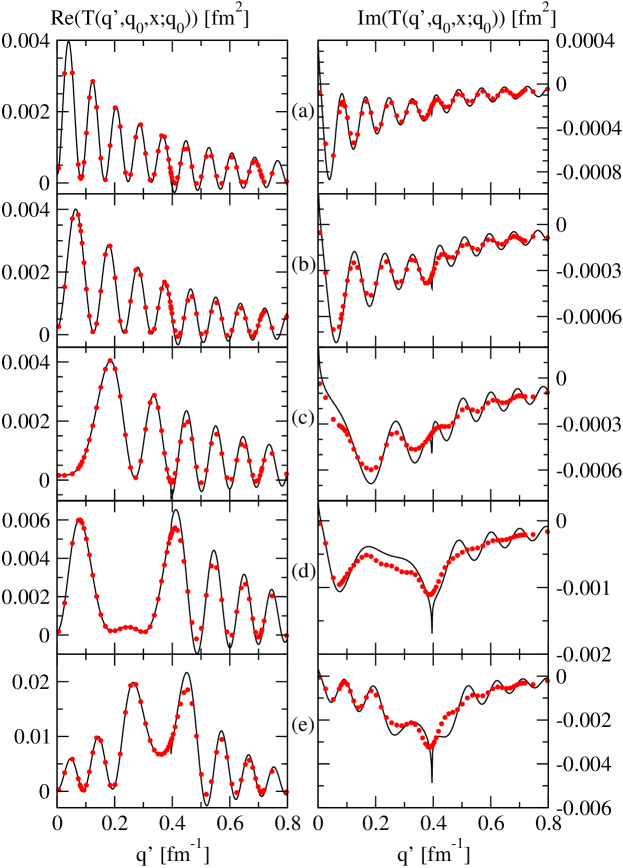
Figure 3: (color online) The real (left) and imaginary (right) part of the half-shell t-matrix $T(q^{\prime},q_{0},x;\,q_{0})$ for the sharply cut-off Coulomb potential with the cut-off radius $R=80$ fm. The solid (black) line represents the asymptotic analytical expression given in (82) and (85). The (red) dots show our numerical results. From top to bottom five different values of $x$ are chosen: (a) $x=-0.91$, (b) $x=-0.50$, (c) $x=0.03$, (d) $x=0.62$, (e) $x=0.90$.

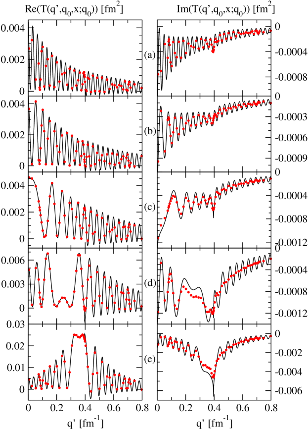
Figure 4: (color online) The same as in Fig. 3 but with the cut-off radius $R=200$ fm.

IV Summary and conclusions

We investigated the screening limit of the exact analytical three-dimensional half-shell t-matrix for a sharply cut-off Coulomb potential. We used the exact three-dimensional wave function for a sharply cut-off Coulomb potential derived in Gl09 . Our direct three-dimensional approach avoids problems related to the summation of the infinite number of partial wave components. Numerical solutions of the three-dimensional Lippmann-Schwinger equation for large cut-off radii agree fairly well with the asymptotic values.

References

(1) W. Glöckle, J. Golak, R. Skibiński,
H. Witała, Exact three-dimensional wave function and the on-shell t-matrix for
the
sharply cut off Coulomb potential: failure of the standard renormalization
factor. Phys. Rev. C79, 044003 (2009).
(2) J. R. Taylor, A new rigorous approach to Coulomb scattering. Nuovo Cimento B 23, 313 (1974).
(3) L. P. Kok, H. van Haeringen, Importance of Coulomb Effects in Half-Shell Scattering. Phys. Rev. Lett. 46,
1257 (1981).
(4) E. Guth, C. J. Mullin, Momentum Representation of the Coulomb Scattering Wave Functions. Phys. Rev. 83, 667 (1951).
(5) W. F. Ford, Anomalous Behavior of the Coulomb T Matrix. Phys. Rev. 133, B1616 (1964).
(6) W. F. Ford, Limiting Forms of the Screened Coulomb T Matrix. Journal Math. Phys. 7, 626 (1966).
(7) Ch. Elster, J.H. Thomas, and W. Glöckle,
Two-Body T-Matrices without Angular-Momentum Decomposition: Energy and Momentum Dependences. Few-Body Systems 24, 55 (1998).