Abstract

A comparative measurement of timing properties of magnetic-resistant fine mesh R7761-70 and ordinary fast R2083 photomultipliers is presented together with preliminary results on the operation of R7761-70 PMs in magnetic field up to 1100 Gauss. The results were obtained using the proton beam of the MC50 Cyclotron of Korea Institute of Radilogical and Medical Sciences.

The ratio of the effective R7761-70 and R2083 TOF (or timing) resolutions was extracted by using two different methods. The results are $1.05\pm 0.066$ and $1.07\pm 0.062$. The gain of R7761-70 PMs is not affected by magnetic field. The R7761-70 TOF/timing resolution becomes $\sim 8\%$ better at 1100 Gauss if the external field is oriented parallel to the PM axis. The results prove the advantages of the design of the CLAS12 Central Time-of-flight system with fine-mesh photomultipliers in comparison with the “conservative” design based on ordinary R2083 PMs and long bent light guides.

1 Introduction

Initially the Central Time-of-Flight system (CTOF) was considered as a barrel made of $\sim 50$ scintillator bars viewed by fast Hamamatsu R2083 photomultipliers (PMs) through $\sim 1.5-1.7$ m long bent light-guides[1, 3] (left panel of Fig. 1). The light guides are to deliver scintillation light to the regions outside the central solenoid where the magnetic field drops down to 300 - 1000 Gauss. Being properly shielded, ordinary photomultipliers are expected to operate in this field.

Problems of this design are obvious:

• The long and bent light guides would deliver a small portion of scintillation light to PMs thus deteriorating the time-of-flight (TOF) resolution;

• The mechanic construction would be rather complicate, ugly, and fragile. It would interfere with other CLAS12 sub-detectors;

• $\sim 100$ long light guides and $\sim 100$ magnetic shields would significantly increase the overall CTOF weight and costs;

The Nuclear Physics Group of Kyungpook National University, in collaboration with Inisitute for Nuclear Research, Moscow, suggests another solution based on magnetic-resistant fine-mesh photomultipliers. Fine-mesh photomultipliers can operate in magnetic field up to 1.5 Tesla. They could be placed closer to scintillator bars at positions where the magnetic field is 0.3 - 1 Tesla (right panel of Fig. 1). The light guides would be much shorter, $\sim 0.50-0.8$ m long, and not bent. No shields would be needed. The CTOF assembly would be simpler, more reliable, and less expensive. A critical question is whether the acceptable TOF resolution could be achieved with fine-mesh of photomultipliers in comparison with R2083 PMs, and how it would be affected by the magnetic field

There was some skepticism regarding fine-mesh photomultipliers. The authors of Ref. [3] wrote that “…While the transition time spread (TTS) is compatible to TTS of R2083, its anode rise time (Rem. of a fine-mesh photomultiplier) is 4 times larger. Therefore it is unlikely it may be used for precise timing…”. Our consideration is different: the real PM anode rise time in a scintillation counter depends also on the light decay constant of a scintillator material. For Bicron-408 it is 2.5 ns - is much longer than the internal R2083 rise time. The most critical parameter is the transit time spread (TTS) which is in fact the variation of electron propagation time inside a photomultiplier. The TTS of fine-mesh R7761-70 photomultipliers is $350$ ps. It is better than that of R2083 PMs ($370$ ps) [5].

Figure 1: Two versions of the CTOF design. On the left: “conservative” design with long bent light guides and ordinary R2083 photomultipliers. On the right: CTOF design with fine-mesh photomultipliers with short straight light guides.

The operation of fine-mesh photomultipliers in magnetic field was investigated in Ref. [6, 7, 8]. The outcome of those studies was encouraging: the timing performance of fine-mesh photomultipliers is good and is not affected by magnetic field up to $\sim 0.8$ Tesla. The authors employed fast laser light pulses as a tool to study PM operation. This technique is quite convenient but it doesn’t allow to estimate the CTOF resolution and to judge between two CTOF designs.

Until recently the cosmic-ray tracking was believed to be a main tool for the CTOF R&Ds [3, 4]. The method uses three stacked parallel equidistant counters viewed by six phototubes under study. If a cosmic-ray muon crosses all three counters, the time (or coordinate) of a scintillation in the middle counter is equal to a half of the sum of times/coordinates in the top and bottom counters. This leads to the following relation

$$\tau=\frac{1}{2}(t_{mid1}+t_{mid_{2}})-\frac{1}{4}(t_{top1}+t_{top2}+t_{bot1}+t_{bot_{2}})=0$$ (1)

where $t_{top1}....t_{bot2}$ denote 6 PM signal arriving times derived from TDC readouts. From Eq. 1 one may deduce the effective timing resolution in each PM channel

$$\sigma_{PM}=\frac{2}{\sqrt{3}}\sigma(\tau)$$ (2)

In practice the PM timing resolution is extracted from the width of the peak in the spectrum of $\tau$.

By employing this method, the KNU group measured the effective R7761-70 timing resolution $\sigma_{PMR7761-70\mu}\approx 52$ ps and found it similar to that of R2083 $\sigma_{PM2083\mu}\approx 53$ ps  [9]. The second result is in good agreement with the previous measurement [4] $\sigma_{PM2083\mu}=52ps\pm 1$ ps.

A disadvantage of this technique is that the measured PM arriving times $t_{top1}....t_{bot2}$ are spoiled by time walks of constant-fraction discriminators (CFD). Time walks depend on pulse shapes and especially on pulse heights. The CFD Phillips 715 and Ortec935 used in Ref. [3, 4, 9], generate time walks up to $\pm 50$ps [10]. Due to light attenuation the pulse heights of muons events depend on hit coordinates and track angles. The variation of the corresponding time walks is comparable with the measured PM timing resolution. That is why the results obtained with cosmic rays, require sophisticated corrections and are cut-, electronic-, and analysis-dependent. They can be used only for rough preliminary estimates of the expected TOF resolution.

In this Note, we present another method to study the operation of scintillation counters and photomultipliers using a well-collimated proton beam. The method has been implemented at the MC50 Cyclotron of Korea Institute of Radiological and Medical Sciences. Simultaneously we report the measurement of the TOF resolution of a plastic-scintillation counter equipped with fine-mesh Hamamatsu R7761-70 photomultipliers and compare it with that obtained with ordinary fast Hamamatsu R2083 PMs. We also report our first results on the operation of fine-mesh R7761-70 photomultipliers in the magnetic field up to 1100 Gauss.

2 Fine-mesh photomultipliers

Fine-mesh photomultipliers have been developed for high magnetic-field applications. Their dynode system has a structure of fine-mesh electrodes stacked in close proximity. Such dynodes provide an improved pulse linearity and resistance to external magnetic field [5].

The survey of properties of fine-mesh photomultipliers is given in Table 1 together with those of R2083 PMs. In general, the timing characteristics of the fine-mesh photomultipliers are worse: the anode rise time varies from $2.1$ to $2.7$ ns. For R2083 PMs this number is $0.7$ ns. However the R7761-70 and R5505-70 transit time spreads are better than that of R2083 PMs.

Phototube	R2083	R5505-70	R7761-70	R5924-70
Dynode system	ordinary	fine-mesh	fine-mesh	fine-mesh
Photocathode dia (mm)	39	17.5	27	39
Photocathode type	bialkali	bialkali	bialkali	bialkali
Anode sensitivity (A/lm)	200	40	800	700
Anode rise time (ns)	0.7	2.1	2.5	2.5
Transit time (ns)	16	5.6	7.5	9.5
Transit time	0.37	0.35	0.35	0.44
spread (ns)

Table 1: Characteristics of fine-mesh photomultipliers in comparison with R2083.

Due to geometrical dimensions only R7761-70 and R5924-70 PMs are suitable for CTOF. Among them, R7761-70 PMs were chosen for initial tests because
i) Their timing characteristics are better than those of R5924-70;
ii) Small dimensions allow us to use them at the CTOF upstream ends;
iii) These phototubes are essentially cheaper than R5924-70 PMs.

Hamamatsu Photonics offers H8409-70 assemblies. A H8409-70 assembly consists of a R7761-70 PM, a voltage divider designed for positive HV supply, and a phototube housing. A positive divider necessarily includes a capacitor in the anode circuit that separates the voltage supply from the anode output. This capacitor may deteriorate timing properties and generate some level at high count rates. The geometric dimensions of H8409-70 assembly are larger than those of a single R7761-70 PM because of a phototube housing.

We developed our own voltage divider designed for negative HV. The distribution of potentials in the dynode system was optimized to achieve the best rise time. R7761-70 PMs were optically attached to scintillator bars and wrapped round with isolation tape without any housing. This made it possible to minimize the counter dimensions and to reduce bores of solenoids used in magnetic-field measurements (Section 11).

Figure 2: Typical anode pulses from cosmic-ray muons obtained with R2083 (left) and R7761-70(middle and right).

Typical R7761-70 and R2083 signals are shown in Fig. 2. They correspond to the detection of cosmic-ray muons in a 3 cm thick scintillator counter. The signals were obtained with $HV\sim 2200V$ for R7761-70 PMs and $HV\sim 2500$ V for R2083 PMs. The R7761-70 rise time $\sim 3.2$ ns. It is only slightly worse than that obtained with R2083PMs ($\sim 2.5$ ns). The R7761-70 pulse height reaches $12V/50Ohm$. Such high pulse heights assure the operation of fine-mesh PMs in magnetic field in which the PM gain might be lower.

3 Method and experimental setup

If a long scintillator bar is viewed by two photomultipliers, the PM arriving times $t_{1}$ and $t_{2}$ corresponding to a particle-induced scintillation are defined by the following relations:

$$t_{1}=TOF+x/v+Const\hskip 28.45274ptt_{2}=TOF+(L-x)/v+Const$$ (3)

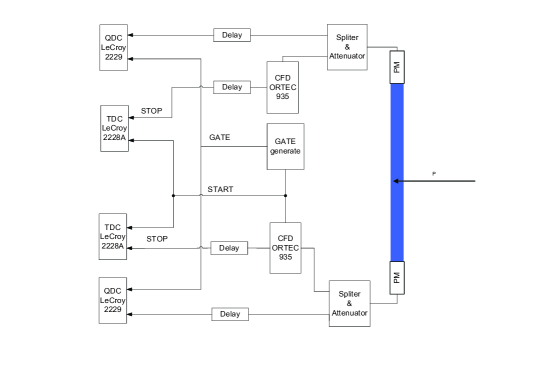
Figure 3: Experimental setup.

where TOF is the time-of-flight of a particle from a certain point (target), $x$ is the coordinate of a scintillation along the counter axis, $L$ is the total length of a bar, $v$ is the efficient speed of light propagation inside a bar, constants originate from cable and electronic delays. Therefore TOF and the coordinate can be derived from the PM times

$$TOF=(t_{1}+t_{2})/2+Const$$ (4)

$$x=v(t_{1}-t_{2})/2+Const$$ (5)

The TOF resolution is

$$\sigma_{TOF}=\sigma((t_{1}+t_{2})/2)=\frac{1}{2}\sqrt{\sigma^{2}(t_{1})+\sigma^{2}(t_{2})}$$ (6)

where $\sigma(t_{1})$ and $\sigma(t_{2})$ are the effective timing resolutions in each PM channel. The variation of the time difference is equal to the TOF resolution

$$\sigma((t_{1}-t_{2})/2)=\frac{1}{2}\sqrt{\sigma^{2}(t_{1})+\sigma^{2}(t_{2})}=\sigma_{TOF}$$ (7)

If a scintillation counter is irradiated by a narrow proton beam, the beam generates a peak in the distribution of events over the coordinate $x$. As it follows from Eq. 5, the coordinate distribution is equivalent to the time-difference spectrum $(t_{1}-t_{2})/2$ scaled by factor $v$. The width of this peak in the time-difference spectrum is defined by the size of the beam spot $\Delta x$ and by the timing performance of the counter

$$\sigma_{peak}=\sigma((t_{1}-t_{2})/2+\Delta x/v)=\sqrt{\sigma_{TOF}^{2}+\sigma(\Delta x/v)^{2}},$$ (8)

where $\sigma(\Delta x/v)$ denotes rms in the coordinate distribution of events due to the finite beam dimension. For a point-like beam $\Delta x\sim 0$

$$\sigma_{peak}\approx\sigma_{TOF}$$ (9)

A well-collimated proton beam allows to derive the TOF resolution by measuring the time-difference spectrum $(t_{1}-t_{2})/2$.

In the practical implementation of this method a counter made of the $50\times 3\times 2$ $cm^{3}$ Bicron-408 plastic scintillator bar was used. The bar was viewed by two photomultipliers under study.

The counter was irradiated by the proton beam of the MC50 Cyclotron of Korea Institute of Radiological and Medical Sciences (KIRAMS). The beam was collimated by a collimator made of 3 stacked together 7 mm thick steel plates. The plates had successively reducing holes of $5,3,$ and $1$ $mm$ diameter in the first, second, and third plates respectively. The plate with the $1$ $mm$ dia hole was attached directly to the 2-cm side of the counter. The whole collimation assembly and the counter were fixed at the end of the beam pipe. As it was deduced from the Geant4 simulations, such collimator reduces the contamination of protons scattered on the collimator walls and minimizes the size of the beam spot.

The PM times $t_{1}$ and $t_{2}$ and their pulse heights $A_{1}$ and $A_{2}$ were digitized by LeCroy 2228B TDCs and LeCroy2229B QDCs and were recorded on-line (Fig. 3). One photomultiplier generated the common TDC START and triggered the acquisition. Both photomultipliers generated the STOP signals for TDCs.

Typically, the beam current was set to $0.15$ nA. At this current the count rate in the counter was $\sim 2\times 10^{4}-10^{5}$ Hz (Sect. 6). The high voltages for fine-mesh R7761-70 PMs were set to low values of $~{}1300-1350$ V, in order to fit QDC ranges.

4 Beam of the MC50 Cyclotron

The MC50 Cyclotron of KIRAMS has been built in 1985 for medical, nuclear-physics, and biological applications. It can produce 20-50 MeV protons and deuterons. A neutron beam line is under construction. Beyond of a medical facility, there are three experimental hatches available for scientific research. The beam spectrum and profile in each hatch depend on the accelerator adjustment, the internal collimators, and other factors. They have to be adjusted for each experiment.

The data reported here were taken as a sequence of short ($\sim 1$ minute) measurements. In total there were 6 beam runs. Among them the data from three last runs are used in this Note. Each beam run lasted two-three days. It included apparatus installation at the MC50 beam line, calibrations, beam adjustment, and main measurements. The beam adjustment was a daily starting point and the most complicated and time-consuming procedure. The beam focusing and the position of the beam spot at the front end of the beam pipe were varied by the accelerator operator. The measured beam light-output spectrum was used as the criterion for the optimization of the beam quality. An example of this procedure is shown in Fig. 4: 8 measured beam spectra correspond to 8 successive steps in the beam tuning. At the final point the set of beam parameters corresponding to the beam spectrum 6 was chosen for the further running.

Figure 4: Procedure of beam adjustment. 8 beam spectra correspond to 8 successive steps in beam tuning. Calibration of the light output $L$ is explained in the Section 5.

The adjusted beam spectrum (the panels 5 and 6 of Fig. 4) exhibits a main peak that corresponds to direct protons, and a tail at lower energies that is produced by particles which were either not properly accelerated or scattered inside the collimator. The position of the peak (i.e. the proton energy) depends on the operating parameters. Usually it was the same while in some cases the peak position was rather different. Such spectrum is shown in the panel 6 of Fig. 4. There the peak position is nearly twice lower than its normal value. Other beam spectra from the runs used in this report are shown in Fig. 7, 8. The calibration of these spectra is explained in the section 5.

5 Birks’ effect and light-output calibration

.

Plastic scintillators do not respond linearly to the ionization density. Very dense ionization columns emit less light than that expected on the basis of $\frac{dE}{dx}$ for minimum ionizing particles. This non-linear response of scintillators is called Birks’ effect [11]. Due to Birks’s effect, protons which stop inside a detector, produce less light per unit of deposited energy than relativistic minimum-ionizing particles.

The semiempirical Birks’ law is

$$\frac{dL}{dx}=L_{0}\frac{\frac{dE}{dx}}{1+k_{b}\frac{dE}{dx}}$$ (10)

where $L$ is the scintillator light production, $L_{0}$ is the specific light production at low ionization densities (i.e. the light produced by a relativistic minimum-ionizing particle per a unit of deposited energy), $x$ is a coordinate along the particle track inside a scintillator volume, and $k_{b}$ is Birks’ constant which must be determined for each scintillator experimentally. An interpretation of Birks’ effect was proposed by C.Chou [12]. He corrected Birks’ formula as

$$\frac{dL}{dx}=L_{0}\frac{\frac{dE}{dx}}{1+k_{b}\frac{dE}{dx}+k_{c}(\frac{dE}{dx})^{2}}$$ (11)

where $k_{b}$ and $k_{c}$ are adjustable constant.

One can write Birks’ law in the general form

$$\frac{dL}{dx}=k_{p}(E)L_{0}\frac{dE}{dx}$$ (12)

where $k_{p}(E)$ is the Birks’s coefficient that depends on $E$, on scintillator material, and on the type of a particle.

Low-energy particles generate less light than relativistic minimum-ionizing (MI) particles. With the increase of the particle energy ($\beta\to 1$), the ratio of light production to deposited energy asymptotically approaches a constant value $L_{0}$ which is the same for all particles. The latter is clear, for example, from the bi-dimensional plots light-output vs TOF for charged pions and protons obtained with the forward lead-scintillator TOF wall [17] at the GRAAL facility. It is convinient to assign this value to $L_{0}=1$. In this case the energy deposited by a minimum-ionizing particle in a detector volume can be used as a measure for light output.

TOF resolution depends on the number of photoelectrons produced at PM photocathodes. The latter is proportional to light output. The CTOF R&D requires to extrapolate the results obtained with the MC50 protons to those expected for fast minimum-ionizing particles. That is why the proton light output was calibrated by assigning it to the light output produced by high-energy cosmic-ray muons.

The muon spectrum was measured just before and/or just after beam measurements. Schematic view of this measurement is shown in Fig. 5. The counter was disattached from the beam pipe and turned at $90^{\circ}$ such that the effective counter thickness of 3 cm was the same for the muons and the beam protons. The count rate of muon events is essentially lower than the background in the experimental hutch. To reject this background, the second similar counter was placed $35$ cm below the main counter. The coincidence of four signals from two counters was requested to trigger the acquisition. This made it possible to select on-line mostly those events in which a cosmic-ray muon passes both counters (Fig. 5).

Beam protons stop inside the counter and totally deposit their energies in the counter volume. Fast muons pass through the counter and act as minimum-ionizing particles. Their energy depositions depend on the track length inside the counter, i.e. on the angle between the muon trajectory and the counter surface.

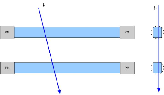
Figure 5: Schematic two-side view of the calibration measurement with cosmic-ray muons.

Two samples of the muon spectra are shown in Fig. 6. They contain the asymmetric peak with the maximum at $\sim 6$ MeV. This maximum corresponds to the energy deposited by a minimum-ionizing particle crossing the counter in the perpedicular direction. The higher-energy part is formed by those muons which cross the counter at smaller angles.

The light output can be derived from the QDCs readouts $A_{1}$ and $A_{2}$ after the pedestal subtraction as

$$L=C\sqrt{(A_{1}-ped_{1})(A_{2}-ped_{2})}$$ (13)

where $C$ is the calibration coefficients that relates QDC channels to the light output. The pedestals were measured by delaying the QDC gates for $~{}200$ ns. The calibration coefficient $C$ was obtained by comparing the measured muon spectrum with the simulated spectrum of the energy deposited by muons (Fig. 6).

Figure 6: Calibrated muon light-output spectra (Data from January 6, 2009). On the left: the spectrum obtained with fine-mesh R7761-70 photomultipliers. On the right: the spectrum obtained with ordinary R2083 photomultipliers. Solid lines are simulated spectra of energy deposited by muons.

As a cross-check, this calibration was applied to the data collected in the same beam run (January 6, 2009) with two counters. One counter was equipped with fine-mesh photomultipliers and the other with ordinary R2083 PMs. The data were collected one-by-one keeping fixed the beam tuning. The muon spectrum with R7761-70 photomultipliers was collected just before the beam run while the one with R2083 PMs was taken immediately after. Both muon spectra are shown in Fig. 6. The calibration coefficients extracted from the muon spectra were then used to reconstruct the beam spectra.

Figure 7: Beam spectra measured with the two different counters (Data from January 6 2009). On the left: the spectrum obtained with fine-mesh R7761-70 photomultipliers. On the right: the spectrum obtained with ordinary R2083 photomultipliers.

The results are shown in Fig. 7. The beam peaks are located at the similar positions near 31.5 MeV. This proves the quality of the calibration procedure. The value of 31.5 MeV corresponds to the light output produced by a minimum-ionizing particle that deposit $\Delta E=31.5$ MeV in the counter volume. The beam protons stop inside the counter and deposit more energy, but, due to Birks’ effect, generate the same light output.

The position of the peak in the spectrum taken next day (January 7 2009) is essentially lower, about $\sim 17.5$ MeV (the panel 6 of Fig. 4). This fact illustrates the importance and the influence of the MC50 beam tuning.

Figure 8: Beam spectra measured in October and November 2008. On the left: the spectrum obtained with fine-mesh R7761-70 photomultipliers (October 2008). On the right: the spectrum obtained with ordinary R2083 photomultipliers (November 2008).

The other beam spectra from the beam runs used in this report (October and November 2008) are shown in Fig. 8. The peaks are located at $L\approx 31.5$ MeV. However the shapes of these spectra are different: the peak is wider and is smoothly continued by the low-energy tail. The reason for this difference still has to be understand. Our assumption is the internal MC50 beam collimator was removed during October/November 2008 beam runs. The data from October/November 2008 were found suitable to retrieve the dependence of the time-of-flight resolution on the light output (Sect. 9).

6 Count rate

Figure 9: Beam spectra in logarithmic scale. The legend is the same as in Fig. 7.

The count rate in the counter depends on the beam current and tuning. In the measurements presented in this Note, the beam current was set to its lowest possible value $0.15$ nA. The count rate can be estimated from the contamination of pileups in the beam spectrum. The probability that two pulses are encoded by QDC as one is

$$P_{pileup}=\frac{N_{pileup}}{N_{tot}}=wN_{cr}$$ (14)

where $N_{pileup}$ is the number of pileup events in a beam spectrum, $N_{tot}$ is the total number of events, $w$ is the width of the QDC gates ($100$ ns in our case), and $N_{cr}$ is the count rate in the counter.

Fig. 9 shows a typical beam spectrum in the logarithmic scale. It contains events whose pulse heights are higher than the peak position. These are pileups. The fraction of such events typically varies from 0.2 to 1%. Following Eq. 14, one may estimate the count rate as

$$N_{cr}\approx 2\times 10^{4}-10^{5}Hz$$ (15)

At this count rate and the high voltage $\sim 1300$V the average anode current of R7761-70 photomultipliers was in the range of $1.6-8\mu A$. Some tentative measurements were carried out at higher count rate/average anode current up to $5\times 10^{5}$ Hz/$\sim 40\mu A$.

It is worth noting that Ref. [6] quotes the maximum average anode current (typically $100\mu A$ for R5024-70 PMs ) which must not be exceeded. Beyond this limit the PM gain is expected to sharply drop down. For those two R7761-70 samples used in our tests, no reduction of the gain at the anode current up to $40\mu A$ was observed. More comprehensive tests at high count rates are planned for 2009.

7 Getting TOF resolution

An example of the measured $(t_{1}-t_{2})/2$ spectrum is shown in Fig. 10. The spectrum contains a narrow peak generated by the beam protons. The width of the peak can be extracted by means a Gaussian fit of this peak. However, because of the limited TDC resolution of $\sim 47$ ps/ch, the result is quite sensitive to the histogram binning. We found critical to set the width of the histogram bins equal to the discreetness of $(t_{1}-t_{2})/2$, i.e. equal to a half of the width of one TDC channel $47ps/2$.

To cross-check the results, another method was employed as well. The center of the peak gravity $M_{peak}$ and the mean square deviation $\sigma_{peak}$ were directly calculated from the sample of collected events as

$$M_{peak}=\frac{1}{N_{ev}}\sum_{i=1}^{N_{ev}}x_{i}$$ (16)

$$\sigma_{peak}=\sqrt{\frac{1}{N_{ev}}\sum_{i=1}^{N_{ev}}(M_{peak}-x_{i})^{2}},$$ (17)

where $N_{ev}$ denotes the total number of selected events, $x_{i}$ is the time difference derived from the TDC readouts $ch_{tdc1_{i}}$ and $ch_{tdc2_{i}}$ for each recorded event as

$$x_{i}=r(ch_{tdc1_{i}}-ch_{tdc2_{i}}).$$ (18)

Here $r$ denotes the TDC scale (i.e. the width of one TDC channel). In the data analysis it was fixed to $r=47ps/ch$. In reality $r$ is affected by the TDC differential non-linearity. For the LeCroy2228B TDC unit used in these measurements, it was measured and found varying from $45$ to $49ps/ch$. This variation leads to systematic uncertainty in each measurement. The way to estimate and to reduce it is explained in the Section 8.

Figure 10: Example of $(t_{1}-t_{2})/2$ spectrum. Gaussian fit of the peak is one of the ways to extract the TOF resolution.

The width of the peak is in fact the combination of the TOF and electronic resolutions.

$$\sigma_{peak}=\sqrt{\sigma_{TOF}^{2}+\sigma_{electronics}^{2}}$$ (19)

The electronic resolution $\sigma_{electronics}$ mostly originates from the TDCs resolution. It was estimated from the spectrum of $\frac{t_{1}}{2}$ in which the same PM signal generates the common START for the TDC and the delayed STOP (Fig. 3). In fact, 99% of events in this spectrum were located in a single channel. The resulting value is $\sigma_{electronics}\sim 6.9$ ps. The corresponding corrections were implemented following Eq. 19.

Both methods were verified in simulations. The values $t_{1}$ and $t_{2}$ were simulated event-by-event using random generators. The generator for $t_{1}$ imitated the measured $t_{1}$ spectrum while the $t_{2}$ generator was Gaussian. The width of the Gaussian distribution is equal to $2\sigma_{TOF}$.

The generated $t_{1}$ and $t_{2}$ values were then digitized in accordance with the discrete scale of LeCroy2228B TDC and recorded in the same format as the experimental data files. The experimental and simulated data were analyzed using the same codes. The simulated TOF resolution was reconstructed with the accuracy of $0.1$ ps in the case of direct calculation and $0.3$ ps using the Gaussian fit.

One well-known problem of timing measurements is the effect of time walks of constant-fraction discriminators (CFD). CFDs generate additional time shifts (time walks) which depend on pulse heights. To extract the TOF resolution, the events were always selected using the criterion

$$L_{i}\leq\sqrt{(A_{1}-ped_{1})(A_{2}-ped_{2})}\leq L_{i+1}$$ (20)

such that the pulse heights $A_{1}$ and $A_{2}$ of the selected events are nearly constant (for example, events from the beam peak). Therefore the influence of time walks on was minimized.

8 TOF resolution with fine-mesh R7761-70 photomultipliers in comparison with R2083 PMs

In this section we report a comparative measurement of the TOF resolutions of two similar counters. One counter was equipped with fine-mesh R7761-70 photomultipliers, and the other with R2083 PMs. Both counters were made of $2\times 3\times 50cm^{3}$ Bicron408 scintillation bars. The photomultipliers were directly attached to the bar butts. The diameter of the photocathodes of R7761-70 photomultipliers, of 27 mm, covered only $\sim 80\%$ of the butt surfaces of the ends of the scintillator bar. Therefore the light collection in this counter was lower by factor $~{}0.8$ than in the case of R2083 PMs.

The beam irradiated the counters at their centers in the direction perpendicular to the counter axis. The TOF resolution of both counters was measured at the same conditions: after the beam adjustment the counters were attached one-by-one to the collimation system. The replacement of the counters took few minutes. During that short break the beam was off. However, the beam parameters were kept fixed. The beam spectra and the count rates were similar in both measurements (Fig. 7). To avoid the effect of the TDC differential non-linearity, the TOF resolution of each counter was measured successively six times. The scheme of the first measurements is shown in Fig. 3. In the second measurement the signal of that PM which does not trigger the acquisition, was additionally delayed for $1$ ns. In the third measurement the delay was 2 ns. Then the PMs were switched and the series of the measurements with additional 0, 1, and 2 ns delays was repeated.

The data were analyzed in an identical way: the same codes was running over the data files corresponding to 12 ($6\times 2$) measurements. Only events from the beam-peak area $31.5MeV\leq L\leq 32.5MeV$ were selected to extract the TOF resolutions.

The results were obtained by using both the direct calculation and the fitting of $(t_{1}-t_{2})/2$ spectra. They are summarized in Table 2 and Table 3. The TOF resolution obtained with R7761-70 PMs was in addition scaled by factor $\sqrt{0.8}$ (last columns of Table 2, 3) in order to account for 80% light collection due to the smaller diameter of the R7761-70 photocathodes. Such “effective” TOF resolution corresponds to the same number of photoelectrons produced at the R7761-70 and R2083 photocathodes. Further the corrected R7761-70 TOF resolution is used for the comparison with R2083 PMs.

Measurement	$PM_{trigger}$	Additional	$\sigma_{TOF_{R2083}}$	$\sigma_{TOF_{R7761-70}}$	$\sigma_{TOFcor_{R7761-70}}$
		delay (ns)
1	1	0	18.85	23.84	20.74
2	1	1	19.09	19.84	17.26
3	1	2	16.14	19.70	17.14
4	2	0	16.30	21.68	18.86
5	2	1	16.43	22.56	19.64
6	2	2	17.60	18.59	16.17

Table 2: TOF resolutions (ps) of R2083 and R7761-70 PMs directly calculated from the samples of collected events

Measurement	$PM_{trigger}$	Additional	$\sigma_{TOF_{R2083}}$	$\sigma_{TOF_{R7761-70}}$	$\sigma_{TOFcor_{R7761-70}}$
		delay (ns)
1	1	0	18.25	22.67	20.28
2	1	1	19.02	19.67	17.50
3	1	2	15.76	19.19	17.16
4	2	0	16.72	20.92	18.70
5	2	1	15.97	22.00	19.68
6	2	2	16.88	18.33	16.40

Table 3: TOF resolutions (ps) of R2083 and R7761-70 PMs obtained using Gaussian fits.

The statistical error of each measurement was $\sim 0.1$ ps. The systematic uncertainty mostly arises from the TDC differential non-linearity. It can be estimated as the deviation of six measured data points from their mean value

$$\sigma_{TOF_{mean}}=\frac{1}{6}\sum_{i=1}^{6}\sigma_{TOF_{i}}$$ (21)

$$\Delta\sigma_{TOFsyst}=\sqrt{\frac{1}{6}\sum_{i=1}^{6}(\sigma_{TOF_{i}}-\sigma_{TOF_{mean}})^{2}}$$ (22)

The estimates for the systematic error in one measurement is $\Delta\sigma_{TOFR2083syst}=1.21$ ps and $\Delta\sigma_{TOFR7761-70syst}=1.58$ ps for the direct calculation method, and $\Delta\sigma_{TOFR2083syst}=1.17$ ps and $\Delta\sigma_{TOFR7761-70syst}=1.38$ for the Gaussian fit. The error for the average of 6 measurements should be scaled by $\frac{1}{\sqrt{6}}$. The averages for the R2083 resolution and for the corrected R7761-70 resolution are

$$\sigma_{TOFR2083}=17.4\pm 0.49{\hskip 28.45274pt}\sigma_{TOFR7761-70}=18.3\pm 0.64$$ (23)

for the direct calculations and

$$\sigma_{TOFR2083}=17.1\pm 0.48{\hskip 28.45274pt}\sigma_{TOFR7761-70}=18.3\pm 0.56$$ (24)

The ratio of the R7761-70 and R2083 resolutions is

$$\frac{\sigma_{TOFR7761-70}}{\sigma_{TOFR2083}}=1.05\pm 0.066$$ (25)

and

$$\frac{\sigma_{TOFR7761-70}}{\sigma_{TOFR2083}}=1.07\pm 0.062$$ (26)

for the direct calculation and for the Gaussian fits respectively. Further the average of both methods

$$\frac{\sigma_{TOFR7761-70}}{\sigma_{TOFR2083}}=1.06\pm 0.064$$ (27)

is used. This ratio means that, if the number of photoelectrons is the same, the TOF resolution with R7761-70 photomultipliers would be $\sim 6.6\pm 6\%$ worse than in the case of R2083 PMs.

The result proves the good timing performance of R7761-70 PMs. Moreover, this ratio was obtained at low $HV\sim 1300V$ of R7761-70 PMs. It is well known that PM timing properties becomes better at higher HV (see, for example, Ref. [7]). In addition, as it will be discussed in the section 11, $\sigma_{TOFR7761-70}$ might be better in magnetic field.

9 Dependence of TOF resolution on light output

To retrieve the dependence of the TOF resolution on the light output, the sample of collected events was divided into many sub-samples following the criterion

$$L_{i}\leq\sqrt{(A_{1}-ped_{1})(A_{2}-ped_{2})}\leq L_{i+1}$$ (28)

The width of the bins $L_{i+1}-L_{i}$ was $1$ MeV. For each bin the width of the peak $\sigma_{peak}$ was derived using both methods.

Figure 11: Dependence of the measured time-of-flight resolution on the light output. Circles are directly calculated from the sample of collected events. Open squares are the results obtained using the Gaussian fit. Error bars correspond to statistical errors only. Where not visible, the errors bars are smaller than the symbol size. The curve is the fit of experimental data. The difference between two fits corresponding to each data set is not seen in the plot.

The results collected with R7761-70 PMs in the October 2008 are shown in Fig. 11. The data obtained by two methods are consistent. The minor deviation at the lower light output is explained by the increasing contamination of scattered protons. This background differently affects the results obtained by each method.

The data points are well fitted by $\frac{C}{\sqrt{L}}$. The results of the fit are

$$\sigma_{TOF}(L)=\frac{96.9\pm 0.27_{stat}\pm 2_{syst}(ps)}{\sqrt{L(MeV)}}$$ (29)

with $\chi^{2}=2.4$ for the directly calculated data points and

$$\sigma_{TOF}(L)=\frac{97.2\pm 0.36_{stat}\pm 2_{syst}(ps)}{\sqrt{L(MeV)}}$$ (30)

for $\chi^{2}=0.95$ for the Gaussian fit. The systematic uncertainty of $2$ ps originates from the TDC differential non-linearity and from the accuracy in the determination of the MIP position.

10 Dependence of TOF resolution on coordinate and track angle

The TOF resolution is related to the PM timing resolutions $\sigma_{PM1}$ and $\sigma_{PM2}$ as

$$\sigma_{TOF}=\frac{1}{\sqrt{2}}\sqrt{\sigma_{PM1}^{2}+\sigma_{PM2}^{2}}$$ (31)

where $\sigma_{PM1}$ and $\sigma_{PM2}$ are the effective resolutions in each PM channel. If a scintillation occurs in the middle of a counter, the numbers of light photons that reaches each PM, are equal. Therefore $\sigma_{PM1}=\sigma_{PM2}$. If a scintillation is located near a counter end $\sigma_{PM1}\neq\sigma_{PM2}$. Due to the exponential light attenuation inside a counter the number of photons which reach each photomultiplier is different. This effect may generate the dependence of the TOF resolution on the axis along the counter axis.

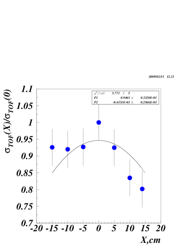
Figure 12: Dependence of the TOF resolution on the coordinate along the counter axis.

To retrieve this dependence, the TOF resolution was measured at different coordinates along the counter axis. The results are shown in Fig. 12. The TOF resolution is $\sim 15\%$ better near the counter ends.

In addition, two measurements were performed with the beam directed at $60^{\circ}$ relative the counter axis. Within the systematic uncertainty, the TOF resolution was the same as that obtained with the perpendicular beam. More accurate data for the $\sigma_{TOF}$ dependence on the coordinate and the angle will be obtained during next beam runs.

11 Operation of R7761-70 PMs in magnetic field

In this section we present first results on the operation of R7761-70 photomultipliers in magnetic field. Both photomultipliers were placed inside air-cooled solenoids. The solenoids were designed and manufactured by the KNU group. They comprise two parallel sections each wounded with 8 layers of 1-mm dia cooper wire. The 5 mm gap between the sections allows the air passage in order to improve the cooling efficiency. In future the number of sections will be increased to 4.

Each section generates 100 Gauss of the magnetic field per 1 A of the current. Due to heating, the maximum current is limited to $\sim 6$ A. Accordingly, the upper limit of the magnetic field in the two-sectional solenoid is 1200 Gauss. Significant increase of the generated field should be expected if the air cooling would be replaced with the water-cooling system.

Figure 13: Dependence of R7761-70 gain on magnetic field.

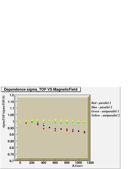
Figure 14: Dependence of R7761-70 TOF resolution on magnetic field.

The measurements were carried out first at 0 Gauss, then at 1100, 1000, 900 …100, and again at 0 Gauss. All the data takings were done at the same conditions one-by-one. The field was varied by changing remotely the solenoid currents.

In total, 4 series of data were taken. In the first series the direction of the magnetic was chosen parallel to the PM axis. In the second series the signal of one PM was additionally delayed for 1 ns. Then the direction of the magnetic field was turned to 180 deg by switching the polarity of the power supply. After that the 3rd and 4th series were done in the similar way.

The results are shown in Fig. 13 and Fig. 14. The gain of R7761-70 PMs was attributed to the position of the beam peak. The beam spectrum in this measurement is shown in the panel 6 of Fig. 4. No any dependence of the gain (i.e. shift in the peak position) on the magnetic field was observed.

Surprisingly, the TOF resolution becomes better if the magnetic field is oriented parallel to the PM axis. The effect reaches $\sim 8\%$ at 1100 Gauss. The antiparallel field does not affect the TOF resolution. This observation has to be checked in next beam runs.

12 CTOF Estimates

In real CTOF assembly most of fast particles will be detected at forward angles. Below we present the estimates of the expected TOF resolution for minimum-ionizing particles emitted from a target at $90^{\circ}$ and $45^{\circ}$.

A minimum-ionizing particles passing through a 3-cm thick counter perpendicular to its axis, deposit $\sim 6$ MeV of energy (Fig. 6). The corresponding TOF resolutions are $\sigma_{TOF_{R2083}}=17.3\sqrt{31.5/6}\approx 39.6$ ps and $\sigma_{TOF_{R7761-70}}=18.3\sqrt{31.5/6}\approx 41.7$ ps for R2083 and R7761-70 PMs respectively.

The scintillation bars in the CTOF assembly will be viewed through light guides. The long bent light guides in the CTOF design with ordinary R2083 PMs (Fig. 1) deliver $\sim 30\%$ of scintillation light [1]. The estimate for the expected CTOF resolution with R2083 PMs would be

$$\sigma_{TOFR2083LG}(90^{\circ})=\sqrt{\frac{1}{0.3}}\times 39.6ps\approx 72.3ps$$ (32)

In the CTOF design with fine-mesh photomultipliers (Fig. 1), the light guides will shorter and not bent. One may assume their light transfer efficiency around $50\%$. The corresponding estimate at $90^{\circ}$ is

$$\sigma_{TOFR7761-70LG}(90^{\circ})=\sqrt{\frac{1}{0.5}}\times 41.7ps\approx 59.0ps$$ (33)

It is essentially better than that number for R2083 PMs.

Minimum-ionizing particles emitted at $45^{\circ}$, deposit $\sqrt{2}$ times more energy in the CTOF counters than ones emitted at $90^{\circ}$. The expected CTOF resolutions are

$$\sigma_{TOFR2083LG}(45^{\circ})=$$ (34)

$${0.85\frac{1}{\sqrt{2}\sqrt{0.3}}\times 39.6ps\approx 43.5ps}$$

$$\sigma_{TOFR7761-70LG}(45^{\circ})=$$ (35)

$${0.85\frac{1}{\sqrt{2}\sqrt{0.5}}\times 41.7ps\approx 35.4ps}$$

where the factor $0.85$ originates from the dependence of the TOF resolution on the coordinate.

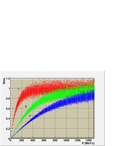
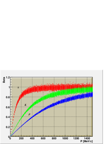
Figure 15: Simulated particle identification in the CTOF detector with fine-mesh R7761-70 photomultipliers at $90^{\circ}$(left) and $45^{\circ}$(right).

The simulated particle identification (PID) based on the quoted above estimates is shown in Fig. 15. The particle speed $\beta$ is used as an identification parameter

$$\beta=\frac{l_{TOF}}{c\times TOF},$$ (36)

where $l_{TOF}$ is a distance from a vertex point inside a target to a hit point on a counter surface. The simulations include four sources of uncertainties:
i) the TOF resolution and its dependence of the light output;
ii) the coordinate resolution $\sigma_{x}=\sigma_{TOF}\times 15cm/ns$;
iii) CTOF azimuthal granularity;
iv) The reconstruction of the vertex point $\pm 1$ mm.

At $90^{\circ}$ kaons are discriminated from pions up to $\sim 600$ MeV/c. Protons are discriminated from kaons up to $\sim 1000$ MeV/c. In the most critical region near $45^{\circ}$ PID is essentially better: protons are separated from kaons up to $\sim 1400$ MeV/c, and pions from kaons up to $\sim 850$ MeV/c.

13 Summary and future R&Ds at KNU.

The measured ratio of the effective TOF/timing resolutions of R7761-70 and R2083 PMs $\frac{\sigma_{TOFR7761-70}}{\sigma_{TOFR2083}}=1.06\pm 0.064$ proves the advantages of the CTOF design with fine-mesh photomultipliers. This design will be more simple, less expensive, and will provide better performance than the “conservative” design with ordinary R2083 PMs.

More information on the properties of fine-mesh photomultipliers will be obtained in the next beam runs. The R&D program includes:
- measurements of the relative TOF resolution of several counters equipped with R7761-70, R5924-70 and R2083 PMs;
- operation of R7761-70 and R5924-70 photomultipliers in magnetic field up to 0.4 Tesla;
- accurate measurements of the dependence of the TOF resolution on the coordinate and track angle.

At the next stage silicon photomultipliers, micro-channel plates could be tested as well using the same technique. Another option might be the development of a time-of-flight system for the detection of neutrons. The new neutron beam line is currently under construction at the MC50 Cyclotron. It will offer a tool for testing prototype counters of the CLAS12 neutron detector [18].

It is a pleasure to thank Dave Kashy, Cyrill Wiggins, and Volker Burkert for the fruitful and efficient collaboration. Silvia Nicolai helped to present the KNU results at JLAB. Our special thanks to the staff of the MC50 Cyclotron for their assistance during beam runs, and especially June Yong Han for the assistance in solving the problem of the beam tuning. This work was supported by Korea Science and Engineering Foundation.

References

- [1] CLAS12 Techical Design Report,
- [2] http://clasweb.jlab.org/wiki/index.php/Main_Page .
- [3] F.Barbosa, V.Baturin et al.,, “Status and further steps toward the CLAS12 “start”-counter.” CLAS-Note 2006-011.
- [4] V.Baturin et al.,, Nucl.Instrum.Meth. A562:327, 2006.
- [5] “Photomultiplier Tubes”, Hamamatsu Photonics, http://www.hamamatsu.com .
- [6] M.Bonesini et al.,, Nucl.Instrum.Meth.A572:465,2007; M.Bonesini et al., Proceeding of 9th ICATPP Conference on Astroparticle, Particle, Space Physics, detectors and Medical Physics Applications, Villa Erba, Como, Italy, October 17 -21 2005, pg.26.
- [7] V.Grigor’ev et al., Instrum.Exp.Tech.49:679,2006.
- [8] T.Tsujita et al., Nucl.Instrum.Meth.A383:413,1996.
- [9] KNU report at 12 GeV Workshop, Jlab, October 31 2007, http://fermi.knu.ac.kr/slava .
- [10] Ortec935 and Phillipls711 manuals.
- [11] J.B.Birks, Proc. Phys. Soc. A64, 874, 1951; J.B.Birks, “Theory and Practice of Scintillation Counting”, Pergamon Press, Oxford, 1964.
- [12] C.N.Chou, Phys. Rev. 87, 904, 1952.
- [13] Saint-Gobain Crystals Comp. Booklet “Scintillation Products”, pg.11 - 12.
- [14] T.J.Gooding and H.G.Pugh, Nucl.Instr.and Meth. 7, 189, 1960.
- [15] G.Kezerashvilli et al., INR Preprint, 1983.
- [16] M.Hirshchberg et al., IEEE Trans. 99, 511, 1992.
- [17] V.Kuznetsov et al.,, Nucl. Instrum. and Meth. A487, 396, 2002.
- [18] S.Nicolai, Talk at the CLAS12 European Meeting, Genoa, February 25 - 28 2009.