New Approaches To Photometric Redshift Prediction Via Gaussian Process Regression In The Sloan Digital Sky Survey

Abstract

Expanding upon the work of Way & Srivastava (2006) we demonstrate how the use of training sets of comparable size continue to make Gaussian process regression (GPR) a competitive approach to that of neural networks and other least-squares fitting methods. This is possible via new large size matrix inversion techniques developed for Gaussian processes (GPs) that do not require that the kernel matrix be sparse. This development, combined with a neural-network kernel function appears to give superior results for this problem. Our best fit results for the Sloan Digital Sky Survey (SDSS) Main Galaxy Sample using $u$,$g$,$r$,$i$,$z$ filters gives an rms error of 0.0201 while our results for the same filters in the luminous red galaxy sample yield 0.0220. We also demonstrate that there appears to be a minimum number of training-set galaxies needed to obtain the optimal fit when using our GPR rank-reduction methods. We find that morphological information included with many photometric surveys appears, for the most part, to make the photometric redshift evaluation slightly worse rather than better. This would indicate that most morphological information simply adds noise from the GP point of view in the data used herein. In addition, we show that cross-match catalog results involving combinations of the Two Micron All Sky Survey, SDSS, and Galaxy Evolution Explorer have to be evaluated in the context of the resulting cross-match magnitude and redshift distribution. Otherwise one may be misled into overly optimistic conclusions.

1 Introduction

General approaches to calculating photometric redshifts from broad band photometric data have been discussed elsewhere recently (Way & Srivastava, 2006, hereafter Paper I). These involve template based approaches and what are referred to as training-set approaches. In this paper we expand upon the training-set approaches outlined in Paper I using Gaussian processes (GPs). Previously we were limited to training set sizes of order 1000 because a matrix inversion of order 1000$\times$1000 was required for calculating the GPs. Part of the limitation was due to the amount of single thread accessible RAM on our circa 2005 32bit computers, meaning that one could not invert a matrix larger than about $O$(1000$\times$1000) in size at one time within Matlab, our choice for implementing GPs. Today one can now use commodity based 64bit workstations and invert matrices of $O$(20000) within Matlab. However, even this is a small fraction of the total potential size of today’s photometric redshift training sets. For this reason we have developed new non-sparse rank-reduction matrix inversion techniques that allow one to use over 100,000 training samples. From this work we demonstrate that the new rank-reduction methods only require approximately 30-40,000 samples to get the optimal possible fit from GPs on Sloan Digital Sky Survey (York et al., 2000, SDSS) data.

Since Paper I several new approaches to Galaxy photometric redshifts from broad band photometry have come about along with expansion and refinement of previously published methods. Below is a summary of some of these approaches.

Kurtz et al. (2007) have used the Tolman surface brightness test ($\mu$– Photo$Z$) using the relation $\mu$$\approx$(1+$z$)^-4 where $\mu$ is the galaxy surface brightness in the SDSS r band via the 50% Petrosian (1976) radii (petroRad50_r): $\mu$=petroMag_r + 2.5(0.798 + 2log(petroRad50_r)) and the galaxy $r$–$i$ colors to pick the red galaxies this method is intended for. The Petrosian radii may add useful information because of the angular diameter distance relation. We also find this to be the case for GPs as discussed in Section 6 below.

Carliles et al. (2008) have used Random Forests (ensembles of classification and regression trees) to estimate photometric redshifts from the SDSS. Like GPs (see Paper I) this method is also supposed to give realistic individual galaxy photometric redshift error estimates and few or no catastrophic photometric redshift prediction failures. Ball et al. (2008) continue their work using machine learning methods to derive photometric redshifts for galaxies and quasars using the SDSS and the Galaxy Evolution Explorer (GALEX, Martin et al., 2005). In particular, they have made interesting progress in eliminating catastrophic failures in quasar photo-$z$ estimation while bringing down the rms error (RMSE) values. Work by Kaczmarczik et al. (2009) uses astrometric information to break degeneracies in quasar photometric redshifts which may also be applied to other kinds of data.

Wray & Gunn (2008) have taken a Bayesian approach using the SDSS apparent magnitude colors $u$–$g$, $g$–$r$, $r$–$i$, $i$–$z$, surface brightness $\mu_{i}$ in the $i$ band, the Sérsic $n$–index (Sérsic, 1968), and the absolute magnitude $M_{i}$ “corrected” to z=0.1. Some of these quantities are only available from the New York University Value Added Catalog (NYC-VAGC) of Blanton et al. (2005) or calculated from the raw photometry directly. Wang et al. (2008) have used support vector machines (also see Wadadekar, 2005) and kernel regression on a SDSS and Two Micron All Sky Survey (2MASS, Skrutskie et al., 2006) cross-match list.

D’Abrusco et al. (2007) utilized a supervised neural network using a standard multilayer perceptron, but operated in a Bayesian framework on two different SDSS datasets. One of their data sets consists of the SDSS Data Release Five (DR5 Adelman-McCarthy et al., 2007) luminous red galaxy (LRG) sample (Eisenstein et al., 2001), and the other which they term the “General Galaxy sample” includes all objects classified as “GALAXY” in the SDSS. They then break their sample up into two redshift ranges and after some interpolation fit to the residuals they obtain impressive results, especially for the LRG sample (see their Table 4). In a higher redshift study Stabenau et al. (2008) used surface brightness priors to improve their template based scheme for photometric redshifts in the VVDS (Le Fèvre et al., 2004) and GOODS (Giavalisco et al., 2004) surveys.

This certainly does not cover all of the recent work in this field, but is a representative sample to show the intense interest being generated because of near-future large-area multi-band surveys like the Large Synoptic Survey Telescope (LSST Ivezic et al., 2008) and PanStarrs (Kaiser et al., 2002).

We have used a variety of datasets in our analysis which are discussed in Section 2. Discussion of the photometric and spectroscopic quality of the datasets along with other photometric pipeline output properties of interest are found in Section 3. The methods used to obtain photometric redshifts are in Section 4. How to pick the optimal sample size, matrix rank, and inversion method in Section 5. Results are in Section 6 and Conclusions in Section 7.

2 The Sloan Digital Sky Survey, The Two Micron All Sky Survey and The Galaxy Evolution Explorer Datasets

Most of the work herein utilizes the SDSS Main Galaxy Sample (MGS, Strauss et al., 2002) and the LRG sample (LRG Eisenstein et al., 2001) from the SDSS Data Release Three (DR3, Abazajian et al., 2005) and DR5 (Adelman-McCarthy et al., 2007). We include the DR3 to facilitate comparison between the present work and that from Paper I. We also utilize the DR5 to maximize the size of our cross-match catalogs.

For comparison with other work we have cross-matched the SDSS datasets with both the 2MASS extended source catalog and GALEX Data Release 4 (GR4) All Sky Survey photometric attributes. Our method of cross-matching these catalogs has not changed since Paper I except that we now cross-match against the SDSS DR5 instead of the DR3 to increase the size of our catalogs. Many aspects of the SDSS, 2MASS, and GALEX surveys relevant to this work were described in Paper I and hence we will not repeat them here. The only new catalog included since Paper I is the SDSS LRG. The SDSS LRG sample is similar to the SDSS MGS except that it explicitly targets the LRGs. These galaxies have a fairly uniform spectral energy distribution (SED) and a strong 4000 Å break which tend to make calculating photometric redshifts easier than for the MGS (e.g. Padmanabhan et al., 2005) since the training–set contains more homogenous SEDs. Since these galaxies are among the most luminous galaxies in the universe and tend to be found in over dense regions (e.g., clusters/groups of galaxies) they are also good candidates for mapping the largest scales in the universe; see (Eisenstein et al., 2001) for more details.

3 Photometric and redshift quality, morphological indicators and other catalog properties

For SDSS photometric and redshift quality we follow much the same recipe as in Paper I. However, unlike Paper I we refrain from using SDSS photometry of the highest quality (what we referred to as “GREAT”) as we did not see any consistent improvments in our regression fits using this higher quality photometry. We stick with the SDSS photometric “GOOD” flags as defined in Paper I: !BRIGHT and !BLENDED and !SATURATED. See Table 2 in Paper I for a description of the flags. We utilize the same photometric quality flags for the GALEX and 2MASS datasets as described in Paper I, Section 3. We incorporate the same SDSS morphological indicators as in our previous work (See Paper I, Section 3.5). The SDSS casjobs queries used to get the data are the same as those in the Appendix of Paper I except in the case of the LRGs utilized herein which require primtarget=TARGET_GALAXY_RED (p.primtarget & 0x00000020 $>$ 0) instead of primtarget=TARGET_GALAXY (p.primtarget & 0x00000040 $>$ 0) for the MGS.

Tables 1 and 2 contain a comprehensive list of the six data sets used herein.

Table 1: Data Sets 1-3

Data Set 1	Data Set 2	Data Set 3
SDSS-DR3 MGS	SDSS-DR5 LRG	SDSS-DR3 MGS + GALEX-GR4
Training=180045,Testing=20229	Training=87002,Testing=9666	Training=30036,Testing=3374
$g$-$r$-$i$	$g$-$r$-$i$	$g$-$r$-$i$
$u$-$g$-$r$-$i$	$u$-$g$-$r$-$i$	$u$-$g$-$r$-$i$
$g$-$r$-$i$-$z$	$g$-$r$-$i$-$z$	$g$-$r$-$i$-$z$
$u$-$g$-$r$-$i$-$z$	$u$-$g$-$r$-$i$-$z$	$u$-$g$-$r$-$i$-$z$
…	…	nuv-fuv-$g$-$r$-$i$
…	…	nuv-fuv-$u$-$g$-$r$-$i$
…	…	nuv-fuv-$g$-$r$-$i$-$z$
…	…	nuv-fuv-$u$-$g$-$r$-$i$-$z$
$u$-$g$-$r$-$i$-$z$-p50	$u$-$g$-$r$-$i$-$z$-p50	nuv-fuv-$u$-$g$-$r$-$i$-$z$-p50
$u$-$g$-$r$-$i$-$z$-p50-p90	$u$-$g$-$r$-$i$-$z$-p50-p90	nuv-fuv-$u$-$g$-$r$-$i$-$z$-p50-p90
$u$-$g$-$r$-$i$-$z$-p50-p90-ci	$u$-$g$-$r$-$i$-$z$-p50-p90-ci	nuv-fuv-$u$-$g$-$r$-$i$-$z$-p50-p90-ci
$u$-$g$-$r$-$i$-$z$-p50-p90-ci-qr	$u$-$g$-$r$-$i$-$z$-p50-p90-ci-qr	nuv-fuv-$u$-$g$-$r$-$i$-$z$-p50-p90-ci-qr
$u$-$g$-$r$-$i$-$z$-p50-p90-fd	$u$-$g$-$r$-$i$-$z$-p50-p90-fd	nuv-fuv-$u$-$g$-$r$-$i$-$z$-p50-p90-fd
$u$-$g$-$r$-$i$-$z$-z-p50-p90-fd-qr	$u$-$g$-$r$-$i$-$z$-p50-p90-fd-qr	nuv-fuv-$u$-$g$-$r$-$i$-$z$-p50-p90-fd-qr

Table 2: Data Sets 4-6

Data Set 4	Data Set 5	Data Set 6
SDSS-DR5 LRG + GALEX-GR4	SDSS-DR5 MGS + 2MASS	SDSS-DR5 LRG + 2MASS
Training=4042,Testing=454	Training=133947,Testing=15050	Training=39344,Testing=4420
$g$-$r$-$i$	$g$-$r$-$i$	$g$-$r$-$i$
$u$-$g$-$r$-$i$	$u$-$g$-$r$-$i$	$u$-$g$-$r$-$i$
$g$-$r$-$i$-$z$	$g$-$r$-$i$-$z$	$g$-$r$-$i$-$z$
$u$-$g$-$r$-$i$-$z$	$u$-$g$-$r$-$i$-$z$	$u$-$g$-$r$-$i$-$z$
nuv-fuv-$g$-$r$-$i$	$g$-$r$-$i$-$j$-$h$-$k$	$g$-$r$-$i$-$j$-$h$-$k$
nuv-fuv-$u$-$g$-$r$-$i$	$u$-$g$-$r$-$i$-$j$-$h$-$k$	$u$-$g$-$r$-$i$-$j$-$h$-$k$
nuv-fuv-$g$-$r$-$i$-$z$	$g$-$r$-$i$-$z$-$j$-$h$-$k$	$g$-$r$-$i$-$z$-$j$-$h$-$k$
nuv-fuv-$u$-$g$-$r$-$i$-$z$	$u$-$g$-$r$-$i$-$z$-j-h-k	$u$-$g$-$r$-$i$-$z$-$j$-$h$-$k$
nuv-fuv-$u$-$g$-$r$-$i$-$z$-p50	…	…
nuv-fuv-$u$-$g$-$r$-$i$-$z$-p50-p90	…	…
nuv-fuv-$u$-$g$-$r$-$i$-$z$-p50-p90-ci	…	…
nuv-fuv-$u$-$g$-$r$-$i$-$z$-p50-p90-ci-qr	…	…
nuv-fuv-$u$-$g$-$r$-$i$-$z$-p50-p90-fd	…	…
nuv-fuv-$u$-$g$-$r$-$i$-$z$-p50-p90-fd-qr	…	…

4 Improved Gaussian Process Methods

In this section we will discuss our investigation of different GP transfer functions (kernels) & rank-reduction matrix inversion techniques. Our results suggest that there may be an upper limit to the number of training-set galaxies needed to derive photometric redshifts using the SDSS, but this result should be viewed with caution. While there have been recent suggestions that one may quantify the maximum number of galaxies required to obtain an optimal fit (Bernstein & Huterer, 2009), in practice what we see with the GPs could be an artifact of the algorithm itself. In particular, it might be desirable to explore building good “local” models to compare with the present GPs (and neural networks), which are global models.

In the GP method utilized herein one would begin with a training set matrix $X$ of dimensions $n\times d$, where $n$ is the number of galaxies and $d$ is the number of components which might include broad band flux measurements and morphological information. One would also have a target vector $y$ of dimensions $n\times 1$, which would contain the known redshift for each galaxy in our case. The testing data are in a matrix $X^{*}$ of dimension $n^{*}\times d$ with target values in a matrix $y^{*}$ consisting of $n^{*}\times 1$ redshifts, where $n^{*}$ is the number of test samples. We wish to predict the value of $y^{*}$ given as $X$, $y$, and $X^{*}$. The prediction of $y^{*}$ requires a covariance function $k(x,x^{\prime})$, with $x$ and $x^{\prime}$ vectors with $d$ components. This covariance function can be used to construct a $n\times n$ covariance matrix $K$, where $K_{ij}=k(x_{i},x_{j})$ for rows $x_{i}$ and $x_{j}$ of $X$, and the $n^{*}\times n$ cross covariance matrix $K^{*}$ ($K^{*}_{ij}=k(x^{*}_{i},x_{j})$ where $x^{*}_{i}$ is the $i$th row of $X^{*}$). Once this is accomplished, the prediction $\hat{y}^{*}$ for $y^{*}$ may be given by the GP equation (Rasmussen & Williams, 2006, p. 17):

$$\hat{y}^{*}=K^{*}(\lambda^{2}I+K)^{-1}y$$ (1)

where $\lambda$ represents the noise in $y$ and can be used to improve the quality of the model (Rasmussen & Williams, 2006).

In addition to the prediction $\hat{y}^{*}$, the GP approach also leads to an equation for $C$ the covariance matrix for the predictions in equation 1. If the $n^{*}\times n^{*}$ matrix $K^{**}$ has entries $K^{*}_{ij}=k(x^{*}_{i},x^{*}_{j})$ then (Rasmussen & Williams, 2006, p. 79):

$$C=K^{**}-K^{*}(\lambda I+K)^{-1}K^{*T}$$ (2)

The superscript $T$ indicates the transpose. The pointwise variance of the prediction is diag($C$), the diagonal of the $n^{*}\times n^{*}$ matrix $C$.

For details about the selection of $\lambda$, the covariance function (kernel) $k$, hyperparameters in the kernel, and GPR in general see Foster et al. (2009) and Rasmussen & Williams (2006). The following discussion is a summary of Foster et al. (2009). We will use the above notation for the sections that follow.

4.1 Different Kernel choices

In Paper I we relied exclusively on a polynomial kernel, but to investigate the possibility that other kernels might perform better we have tried several other common forms in the meantime.

The squared exponential (SE) kernel function (also known as the ’radial basis’ kernel function) is given by

$$k_{SE}(r)=\exp\left(-\frac{r^{2}}{2l^{2}}\right)$$ (3)

where $l$ is the length scale. The length scale determines the rate at which the kernel function drops to zero away from the origin. This covariance function is infinitely differentiable and hence is very smooth. Because it is so smooth, it can sometimes be unrealistic for use in modeling real physical processes.

The Matern class covariance function is given by

$$k(r)=\frac{2^{l-v}}{\Gamma(v)}\left(\frac{\sqrt{2vr}}{l}\right)^{v}K_{v}\left(\frac{\sqrt{2vr}}{l}\right)$$ (4)

where $v$ and $l$ are positive parameters and $K_{v}$ is a modified Bessel Function. As $v\rightarrow\infty$ this reduces to the SE above. The process becomes very non-smooth for $v=\frac{1}{2}$ and for values of $v\geq\frac{7}{2}$, the function is as rough as noise. The Matern class covariance function is mean square differentiable $k$ times if and only if $v>k$. The Matern class of covariance functions can be used to model real physical processes and is more realistic than the above SE covariance function.

The rational quadratic covariance function is given by

$$k(r)=\left(1+\frac{r^{2}}{2\alpha l^{2}}\right)^{-\alpha}$$ (5)

As the value of the parameter $\alpha\rightarrow\infty$ this reduces to the SE function described earlier. Unlike the Matern class covariance function, this function is mean square differentiable for every value of $\alpha$.

The polynomial covariance function is given by

$$k(x,x^{\prime})=(\sigma_{0}^{2}+x^{T}\Sigma_{p}x^{\prime})^{p}$$ (6)

where $\Sigma_{p}$ is a positive semidefinite matrix and $p$ is a positive integer. If $\sigma_{0}^{2}=0$ the kernel is homogeneous and linear, otherwise it is inhomogeneous. In principle this function may not be suitable for regression problems as the variance grows with $\mid x\mid$ for $\mid x\mid>1$. However there are applications where it has turned out to be effective (Rasmussen & Williams, 2006).

The neural network covariance function is given by

$$k_{NN}(x,x^{\prime})=\frac{2}{\pi}sin^{-1}\left(\frac{2x^{T}\Sigma x^{\prime}}{\sqrt{(1+2x^{T}\Sigma{x})(1+2x^{\prime T}\Sigma x^{\prime})}}\right)$$ (7)

This covariance function is named after neural networks because the function can be derived from the limiting case of a model of a neural network (Neal, 1996)

In our calculations we chose $\Sigma$, which scales as the training-set data, to have the form $I/l^{2}$ where $I$ is a $d\times d$ identity matrix. The hyperparameters $l$ and $\lambda$ were selected by finding a (local) maximum to the marginal likelihood using the routine $minimize$ from Rasmussen & Williams (2006, pp. 112-116, 221).

Two or more covariance functions can be combined to produce a new covariance function. For example sums, products, convolutions, tensor products and other combinations of covariance functions can be used to form new covariance functions. Details are described in Rasmussen & Williams (2006).

For the calculations shown in the rest of the paper we utilized equation 7, the neural network kernel, since for our data it outperformed all other kernels.

4.2 Low Rank Approximation Matrix Inversion Techniques

As mentioned in Paper I (Section 4.4) to utilize GPR the inversion of the matrix $M=(\lambda^{2}I+K)$ in equation 1 is required. This matrix turns out to be an $n\times n$ non-sparse matrix where $n$ is the number of training-set galaxies. Paper I mentioned that matrix inversion requires $O(n^{3})$ floating point operations. Thus, to accommodate the matrix in memory and to keep the computation feasible, we kept $n\leq$1000 in Paper I.

This was a severe shortcoming for GPs since they had 1–2 orders of magnitude less training samples to work with than all of the other methods described in Paper I. Nonetheless, GPs performed extremely well within this limitation.

Since writing Paper I, we have developed a variety of rank-reduction methods to invert large non-sparse matrices. These will make GPR much more competitive than that shown in Paper I. Foster et al. (2009) outline the rank-reduction methods utilized in detail, so we provide a brief summary of their advantages below.

Note that the number of samples, $n$, is the same as that described above, while the rank, $m<n$, is the size of the rank-reduced matrix. We typically keep $m<$1500 to keep the numbers of operations to invert the matrices manageable in wall-clock time. Memory usage for the methods below is $O(nm)$.

SR-N: the subset of regressors method. This method has been proposed and utilized in the past (Rasmussen & Williams, 2006; Whaba, 1990; Poggio & Giroso, 1990) and requires nm² flops to invert. However, this method is known to have problems with numerical stability. That problem is addressed in the methods below.

SR-Q: the subset of regressors using a QR factorization. The use of the QR factorization (Golub & Van Loan, 1996, p.239) is designed to reduce computer arithmetic errors in the SR-N method. This method requires 2nm² flops to invert. Therefore, it is a little more expensive than SR-N.

SR-V: the $V$ method. Since this method in combination with pivoting (see below) is the one we utilize the most in later aspects of this paper we will go into a little more depth here. From Section 4 Equation (1) we recall that the size of $(\lambda^{2}I+K)^{-1}$ is $n\times n$ and as mentioned above for large $n$ it is not practical to calculate $(\lambda^{2}I+K)^{-1}$ directly. To get around this we will approximate $K$ with $VV^{T}$ where $V$ is produced by partial Cholesky factorization (see Foster et al. (2009)). Let $K^{*}_{1}$ be the first $m$ columns of $K^{*}$ and let $V_{11}$ be the $m\times m$ matrix of the first $m$ rows of $V$ where $m<n$. Then let $V^{*}=K^{*}_{1}V^{-T}_{11}$. In addition to replacing $K$ with $VV^{T}$ we can also approximate $K^{*}$ with $V^{*}V^{T}$. With these substitutions one sees that $K^{*}(\lambda^{2}I+K)^{-1}y$ from Equation (1) can be approximated by $V^{*}V^{T}(\lambda^{2}I+VV^{T})^{-1}y$. It turns out that this can also be written as $\hat{y}^{*}=V^{*}(\lambda^{2}I+V^{T}V)^{-1}V^{T}y$. The matrix $(\lambda^{2}I+V^{T}V)^{-1}$ is now $m\times m$ instead of $n\times n$ and for small enough $m$ the equation can be solved quite quickly. The new flop count will be $O$(nm²).

This method is intermediate in terms of growth of computer arithmetic errors between the normal equations and the SR-Q method, but in general the accuracy is close the SR-Q. This method was first discussed by Seeger et al. (2003) and Whaba (1990, p.136).

SR-NP, SR-QP, SR-VP: the use of pivoting with rank-reduction methods. All of the previous methods use the first m columns of $K$, but one can select any subset of the columns to construct a low–rank approximation. Selecting these columns is part of the problem to be solved. Our approach is similar to that of Fine & Scheinberg (2001).

Pivoting is useful in forming a numerically stable low–rank approximation of a positive semi-definite matrix, and to do so it identifies the rows of the training data which limit the growth of computer arithmetic errors. A pivot of the matrix $K$, which is simply a permutation of $K$ of the form $PKP^{T}$ corresponds to the permutation $PX$ of $X$. It is possible to move columns and rows of $K$ so that the $m\times m$ leading principal submatrix of $PKP^{T}$ has the condition number that is a function of $n$ and $m$. Thus pivoting will tend to construct a low–rank approximation whose condition number is related to the condition number of the low–rank approximation produced by the singular–value decomposition. However, the growth of computer arithmetic errors in the algorithm depends on the condition number of the low–rank approximation. Since pivoting limits the condition number and the growth of computer arithmetic errors depends on the condition number, pivoting will tend to improve the numerical stability of the algorithm. This can, in principle, reduce the effect of computer arithmetic errors. If computer arithmetic errors are larger than the other errors (such as measurement errors and modelling errors) in the prediction of the redshift, then an algorithm incorporating pivoting may potentially be more accurate than an algorithm without pivoting.

Examples 2–4 in Foster et al. (2009) illustrate some of the dangers of not pivoting and how they are resolved with pivoting for small (artificial) problems.

In the end adding pivoting increases SR-N to 2nm² flops and SR-Q to 3nm² while SR-V stays the same.

5 Comparison: Picking the optimal Sample Size, Rank size, and Matrix Inversion Method

Here we investigate Data Set 1 in detail in order to discern a variety of things including: is there an optimal sample size for a given survey; what is the best matrix inversion method; if using rank-reduction methods what is the optimal rank size? When discussing conventional matrix inversion, we will be limited to a maximum of 20,000 training samples .

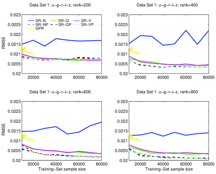
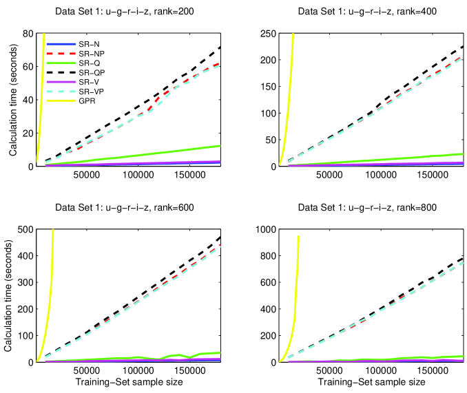
Figures 1 and 2 show the variation of RMSE and calculation time versus sample size. For the GP method (which is labeled GPR and is in yellow), this involved a full matrix inversion up to 20,000 training-set samples. The rest of the curves are from the other rank-reduction matrix inversion techniques and are labeled as described in the previous section. Several features are apparent:

1. The SR-N method does not perform well in comparison to any of the other techniques. However, it does invert its matrices much faster than the standard matrix inversion technique.

2. Except for the SR-N method, all of the other rank-reduction methods outperform the full matrix reduction in the range of 10,000–20,000 samples.

3. The rank-reduction methods with pivoting slightly outperform the non-pivoting methods in term of lower RMSE values. However, the pivoting methods take much more time to do the matrix inversions than the non-pivoting methods.

4. More training-set samples give lower RMSE values. By around 40,000 samples the curves start to level off regardless of the rank size.

5. Larger rank sizes clearly give better performance in terms of lower RMSE for a given sample size. This is described in more detail below.

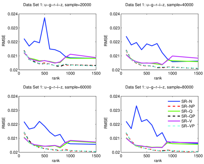
Figure 3 shows the variation of RMSE with rank for several different sample sizes. The rank is plotted from 100 to 1000 in increments of 100, but we also add rank=1500 to see if there is a large change in calculated RMSE for a much larger value. Some important features to note here:

1. As in Figure 1, the RMSE decreases for larger sample sizes, but as was noted earlier, there is not a large difference between sample sizes of 40,000 and above.

2. For the non-pivoting matrix inversion techniques (not including SR-N) SR-Q and SR-V the RMSE increases beyond rank=800. This suggests that there might be some instability associated with non-pivoting methods as rank size becomes large. For this reason, one should stick with the pivoting methods (SR-QP or SR-VP) if one wishes to use a rank of 800 or larger.

3. On average it appears that SR-VP and SR-QP outperform the other rank reduction methods. SR-VP also appears to outperform SR-QP, although the difference is marginal.

4. SR-VP with rank=800 and sample size=40000 appear to be optimal choices for our data when looking at Figures 1–3 given the accuracy of the result. The timings are much longer for these pivoting methods as shown above, but they outperform all other methods.

Figure 1: From Data Set 1 (see Table 1). Error bars are not plotted for reasons of clarity; however, they are of the same order as the scatter in the lines.

Figure 2: From Data Set 1 (see Table 1), but unlike in Figure 1 we show that the matrix inversion times are linear out to the full size (180,000 galaxies) of the data set.

Figure 3: From Data Set 1 (see Table 1) error bars are not plotted for reasons of clarity. They are of the same order as the scatter in the lines.

6 Results

6.1 SDSS Main Galaxy and LRG Results

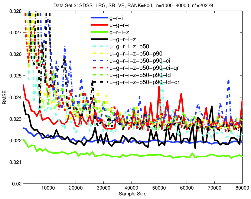
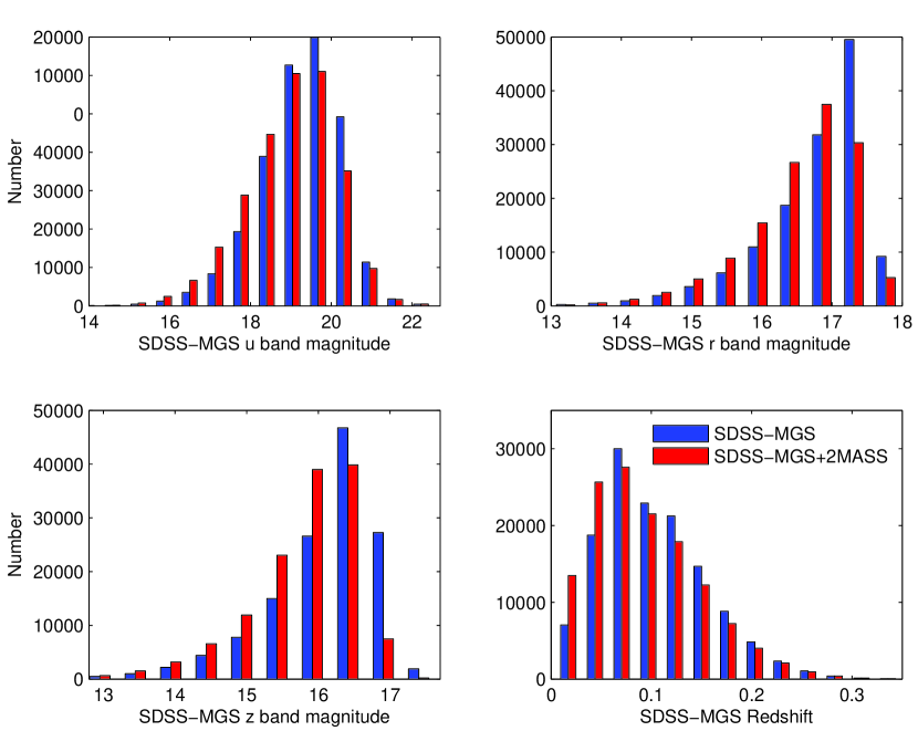
The SDSS MGS (Data Set 1) & LRG (Data Set 2) will give us different results because the LRG sample has far fewer SED types than are found in the SDSS MGS while the LRG sample goes to fainter magnitudes and hence deeper redshifts (see Figures 8 and 9). This will make the job of any regression algorithm quite different. This is evident in the two panels of Figure 4, which show the variation of RMSE versus sample size for the two different data sets. A number of points need to be stressed:

1. $MorphologicalInputs$. The morphological information (p50, p90, ci, fd, qr) may add some information that the regression algorithm can utilize. This includes the Petrosian 50% radii (p50), the Petrosian 90% (p90), the inverse concentration index (ci=p50/p90), the FracDev (fd) and Stokes $Q$ parameter (qr) all in the SDSS $r$ band. More details on these parameters are discussed in Paper I. Data Set 1 (Figure 4(a)) and the five SDSS filters $u$-$g$-$r$-$i$-$z$ (not including morphology inputs) clearly outperform all of the subsets of $u$-$g$-$r$-$i$-$z$ ($g$-$r$-$i$, $u$-$g$-$r$-$i$, and $g$-$r$-$i$-$z$) and the addition of morphological inputs. In Data Set 2 (Figure 4(b)) the morphological information appears to add noise for the most part making the fits worse than by using only combinations of the five SDSS $u$-$g$-$r$-$i$-$z$ bandpass filters.

2. $FewerSEDs$. As mentioned in the previous section, by the time sample sizes of $\sim$ 40,000 are reached in the SDSS–MGS of Data Set 1 (Figure 4(a)) the RMSE begins to level off. In the SDSS–LRG of Data Set 2 (Figure 4(b)) however this is already occurring for most of the inputs in the 10,000–20,000 range. This is clearly the advantage of having less SEDs to worry about in the SDSS–LRG sample versus the SDSS–MGS. In fact for Data Set 2 (SDSS–LRG) it is clear that only four of the five SDSS bandpasses are sufficient for the optimal fit ($g$-$r$-$i$-$z$). The SDSS $u$ bandpass is clearly superfluous in the SDSS–LRG data set when using GP fitting routines.

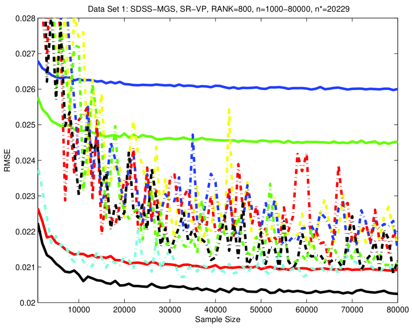
3. $Errors$. 90% confidence levels derived from the bootstrap resampling are roughly at the level of the variation in each of the inputs used as a function of sample size. It is clear that adding morphological information requires larger error estimates for these datasets.

Figure 4: From Data Sets 1 and 2 (see Table 1). We utilize the rank–reduction method termed SR-VP with a rank size of 800. The training sets ($n$ in the plot, following our earlier notation) range in size from 1000 to 80,000 in 1000 increments with 10 bootstraps (Efron & Tibshirani, 1993) per run. The testing sample size ($n^{*}$) was always 20,229. The mean value of the 10 bootstraps is plotted. 90% confidence levels from the bootstrap resampling are of order the vertical line variation. Clearly, the errors are much larger for those which include the morphological parameters.

6.2 Cross-Matching GALEX and SDSS Results

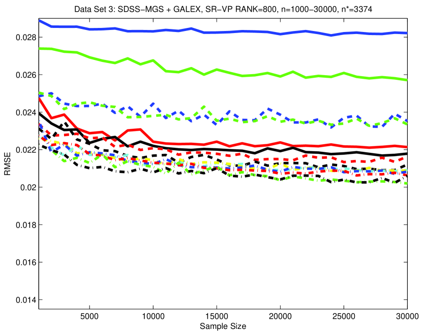
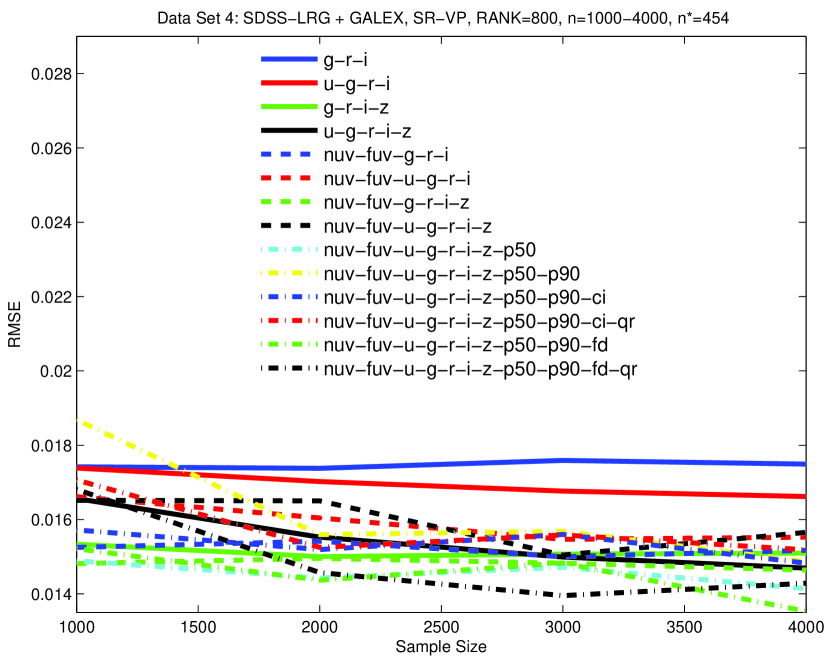
Figure 5 shows results from a cross-match of the SDSS and GALEX catalogs, which are listed as Data Sets 3 and 4 in Tables 1 and 2. Figure 7 shows the SDSS and SDSS + GALEX results for Data Sets 1–4, but without any SDSS morphological inputs included. This is to better quantify the differences between the SDSS and SDSS + GALEX GP fits. The following should be noted:

1. Comparing Figure 4(a) to Figure 5(a) one sees that those inputs that include SDSS morphological information are slightly improved when GALEX filters are included. The error bars on those with morphological inputs (errors not shown here) are also smaller in Figure 5(a) versus Figure 4(a). This would imply that the addition of GALEX filters helps make better use of the morphological inputs.

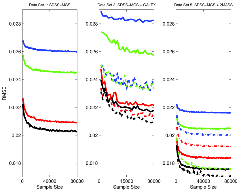
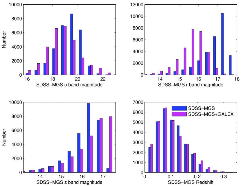
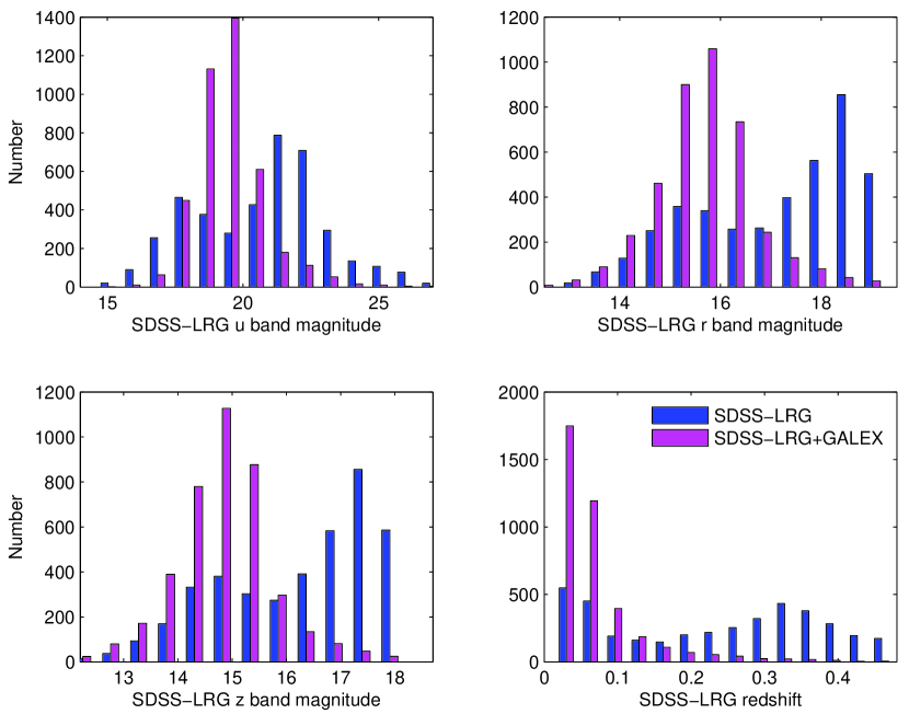
2. Figure 7(a) is made up of Figures 4(a), 5(a), and 6(a) without the SDSS morphological information included. One notices that Data Set 3 (SDSS–MGS + GALEX) in Figure 7(a) has higher RMSE values for the purely SDSS bandpasses ($g$-$r$-$i$, $u$-$g$-$r$-$i$, $g$-$r$-$i$-$z$, $u$-$g$-$r$-$i$-$z$) than Data Set 1 (SDSS–MGS only). Here the max size of the training data sets is different by a factor of 2.7 (80,000 versus 30,000) hence the difference may be attributed to a smaller data set size, although that is unlikely given how we subsample the data in Data Set 1. However, if one examines Figure 8 one sees clear differences and similarities in the magnitude and redshift distributions of these two catalogs. In particular the r-band magnitude distribution is quite distinct, the z-band less so. This seems to have made it harder for the GPs to obtain a good fit for the MGS galaxies. Within Data Set 3 of Figure 7(a) the GALEX bandpasses help with two of the SDSS only input options ($g$-$r$-$i$ and $g$-$r$-$i$-$z$) compared to Data Set 1. However, the two GALEX bandpasses do not help with the best inputs from Data Set 1 ($u$-$g$-$r$-$i$ and $u$-$g$-$r$-$i$-$z$). Hence for the MGS galaxies there appears no need to utilize the GALEX magnitudes to improve photo-z estimation over that already obtained from SDSS only magnitudes. The same applies to the the SDSS morphological information, which adds very little of substance. For example, compare u-g-r-i-z in Data Set 1 (Figure 4(a)) versus nuv-fuv-$u$-$g$-$r$-$i$-$z$-p50-p90-fd-qr in Data Set 3 (Figure 5(a)).

3. Comparing Figures 4(b) and 5(b), one sees that the LRG + GALEX cross-match catalog has lower RMSE values than the LRG only catalog regardless of the inputs used. Hence one would be led to believe that one should always use GALEX magnitudes where available for LRG galaxies to improve photo-$z$ estimation. However, there are two other things to take note of. First, one again sees that the max training data set size is a factor of 20 smaller (80,000 versus 4000) between Data Sets 4 and 2, although Data Set 2 does take a subsample at the level of Data Set 4. Therefore, sample size does not appear to be the issue here. Looking at Figure 9 it is clear that there are few similarities in the magnitude or redshift distributions for these two data sets. Clearly the GP algorithm is fitting a completely different set of data points and it finds Data Set 4 much easier than Data Set 2.

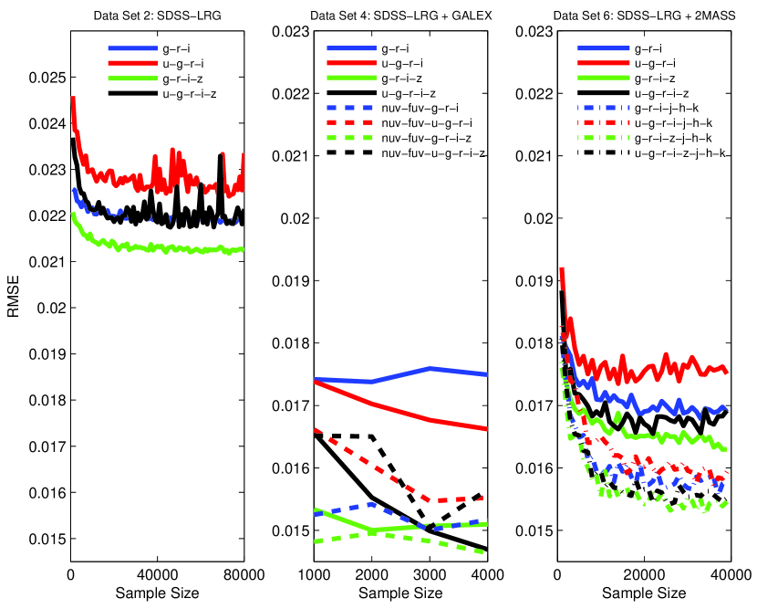
4. Looking at Figure 7(b) (made up of Figures 4(b), 5(b) and 6(b) without the SDSS morphological inputs included) the addition of the GALEX nuv–fuv filters within Data Set 4 seem to assist in photo-$z$ estimation when using SDSS filters $g$-$r$-$i$ and $u$-$g$-$r$-$i$, but has a little effect when added to the already superior $g$-$r$-$i$-$z$ and $u$-$g$-$r$-$i$-$z$.

As noted above, the RMSE differences between Figures 4(a) and 5(a) suggest that the underlying distribution of SDSS magnitudes and redshifts of Data Set 1 versus 3 are different as seen in Figure 8. The data set has shrunk in size between Data Sets 1 and 3, while the redshift distribution appears the same. However, the colors of the galaxies have changed enough that the GPs find it harder with the reduced sample size to obtain a good fit.

The explanation for the improvement seen between Figures 4(b) and 5(b) (Data Sets 2 and 4) is perhaps simpler. Figure 9 shows the $u$,$r$,$z$ and redshift distributions for these two data sets. Clearly, the centroid, spread, and shape of the distributions of the $u$,$r$,$z$ and redshift distributions are signficantly different. The LRG + GALEX redshift distribution in particular is strongly truncated beyond a redshift of about 0.2 while the magnitude distributions tend to be more Gaussian in shape. Certainly it is easier for GPs to come up with better fits for lower-redshift distributions.

The marked differences between the SDSS MGS and LRG results are because of the different galaxy SEDs that exist in each catalog. These differences also exist because the LRG samples go fainter than the MGS samples (see Eisenstein et al., 2001) and they have a different redshift and galaxy magnitude distribution (see Figures 8 and 9). The magnitude and redshift differences between the pure LRG and LRG+GALEX catalogs are much larger than they are between the corresponding MGS and MGS+GALEX catalogs. Clearly the additional GALEX inputs affect the SDSS MGS only ($u$-$g$-$r$-$i$-$z$) results negatively, while the GALEX inputs affect on the LRG sample is ambiguous at best. These differences suggest that one must be very careful in interpreting the improvement in RMSE results associated with any SDSS + GALEX cross-match catalogs.

Figure 5: From Data Sets 3 and 4 (see Table 1). We utilize the rank-reduction method termed SR-VP with a rank size of 800. On the left in plot (a), we use training sets ($n$ in the plot, following our earlier notation) ranging in size from 1000 to 30,000 in 1000 increments with 10 bootstraps per run. The testing sample size ($n^{*}$) is 3374. The mean value of 10 bootstraps resampling runs is plotted. 90% confidence levels from the bootstrap resampling are of order the vertical line variation. On the right, we use similar notation, but we have smaller training (1000–4000 in increments of 1000) and testing (454) sets.

Figure 6: From Data Sets 5 and 6 (see Table 1). We utilize the rank–reduction method termed SR-VP with a rank size of 800. For Data Set 5 the training sets (denoted as $n$) range in size from 1000 to 80,000 in 1000 increments with 10 bootstraps per run and a testing-set ($n^{*}$) size of 15,050. On the right, Data Set 6 training sets range from 1000 to 40,000 in increments of 1000 with 10 bootstraps per run and a testing-set size of 4420. Bootstrap 90% confidence levels are again of order the vertical line variation.

6.3 Cross-Matching 2MASS and SDSS Results

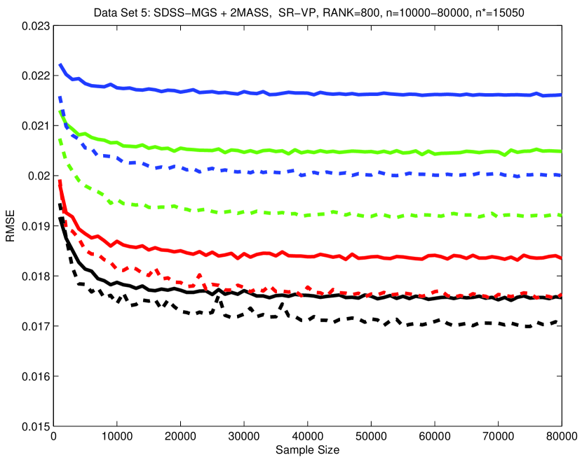
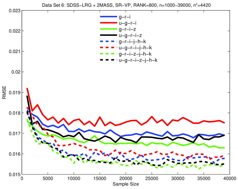
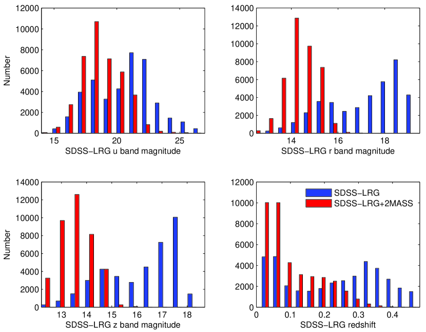
Figure 6 demonstrates our GPR results from a cross-match catalog containing the 2MASS extended source catalog with the SDSS MGS (Data Set 5) and the SDSS LRG sample (Data Set 6). When Figure 6 is compared with Figure 4, the results in Figure 6 are significantly better for both cases. While it might be tempting to attribute this improvement to the inclusion of additional bandpasses in the analysis in Figure 6, it is important to take note of a variety of other important differences between the RMSE estimates in these two figures.

Figure 7: From Data Sets 1–6 (see Table 1). The SDSS $u$-$g$-$r$-$i$-$z$ filter combinations alone along with those of GALEX nuv, fuv filters, and 2MASS $j$,$h$,$k$. This demonstrates how the addition of the GALEX and 2MASS filters influence the SDSS only magnitude fits via the GP SR-VP method.

1. For the SDSS only bandpasses ($u$-$g$-$r$-$i$-$z$) the RMSE drops significantly between Data Sets 1–5 (Figure 4(a) – 6(a)) and Data Sets 2–6 (Figures 4(b) – 6(b)); see Figure 7 for another viewpoint. This drop is because the 2MASS galaxies tend to be brighter and at lower redshift making the cross-match catalog between the 2MASS and SDSS also brigher and lower redshift than the SDSS only catalog especially for the case of the LRG cross-match samples (see Figures 10 and 11).

2. Figure 6(b) (Data Set 6) has lower RMSE values compared to Figure 4(b) (Data Set 2) regardless of input. It also appears to converge to a best fit RMSE very quickly in comparison to Data Set 5 (Figure 6(a)).

3. In Figure 7(a) (focusing on Data Sets 1 and 5) it is clear that adding the 2MASS fluxes improves the RMSE fit regardless of which SDSS filters are combined with the 2MASS $j$-$h$-$k$ bandpasses.

4. In Figure 6(b) (Data Set 6) adding the 2MASS fluxes can improve the RMSE fit, but the conditions under which this improvement occurs are significantly different from those in Figure 6(a) (Data Set 5). Upon close inspection it can be seen that equivalent best results are obtained as the training sample reaches $\sim$ 20,000 using $g$-$r$-$i$-$z$-$j$-$h$-$k$ (dashed green). This shows that for Data Set 6, the $u$ band adds little to the LRG sample. This is consistent with the behavior observed in Figure 4(b) (Data Set 2).

Figure 8: Overlapping histograms for Data Sets 1 and 3 (see Table 1) from three of the five SDSS magnitudes ($u$,$r$,$z$). Data Set 1 is in blue, and Data Set 2 in magenta. Of course, the SDSS+GALEX cross-match catalogs (Data Set 3) are smaller, so the SDSS only data (Data Set 1) was randomly resampled to be the same size as the cross-match catalog so that trends in the plots are directly comparable.

Figure 9: Overlapping histograms for Data Sets 2 and 4 (see Table 1) from three of the five SDSS magnitudes ($u$,$r$,$z$). Data Set 2 is in blue and Data Set 4 in magenta. Of course, the SDSS+GALEX cross-match catalogs (Data Set 4) are smaller, so the SDSS only data (Data Set 2) was randomly resampled to be the same size as the cross-match catalog so that trends in the plots are directly comparable.

Figure 10: Overlapping histograms for Data Sets 1 and 5 (see Table 1) from three of the five SDSS magnitudes ($u$,$r$,$z$). Data Set 1 is in blue and Data Set 5 in red. Of course, the SDSS+2MASS cross-match catalogs (Data Set 5) are smaller, so the SDSS only data (Data Set 1) was randomly resampled to be the same size as the cross-match catalog so that trends in the plots are directly comparable.

Figure 11: Same as Figure 10 except we use Data Sets 2 (blue) and 6 (red)

6.4 Systematics

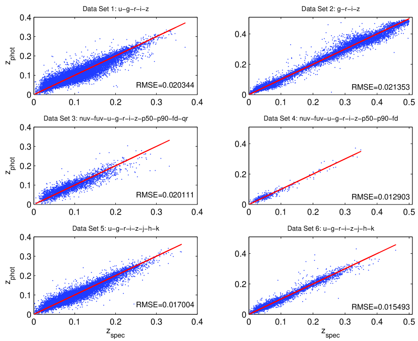
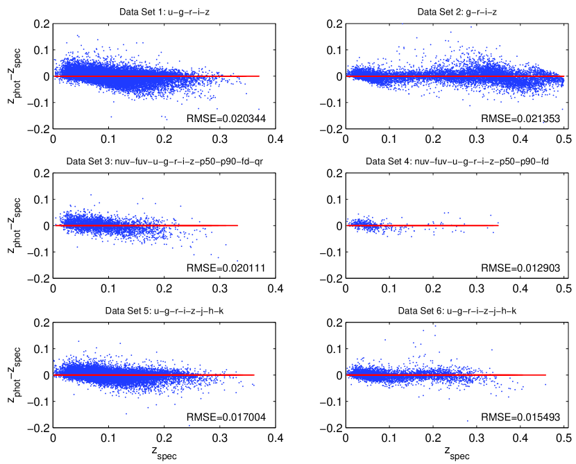
In Figures 12 and 13, we plot the redshifts and residuals, respectively, for those data sets that yield the lowest RMSE. The actual RMSE is also indicated in each plot. There appears to be a systematic shift above the regression line for redshifts less than 0.1 and below the regression line between 0.1$<$z$<$0.2 for Data Sets 1, 3 and 5. This effect has been seen or discussed in many papers on this topic (e.g. Collister & Lahav, 2004; D’Abrusco et al., 2007; Ball et al., 2008; Wang et al., 2009).

At low redshifts (z$<$0.1) the bias in the regression line seen in Figure 12 (Data Set 1) is probably caused by the lack of deep $u$-band data (see Figures 8 and 9). When supplemented by the GALEX data the bias looks to be slightly improved in Data Set 3 (see Figures 12 and 13). The bias seen in between redshifts of 0.1$<$z$<$0.2 for the SDSS-MGS data sets (Data Sets 1,3,5) is probably due to degeneracies in the spectral features of those galaxies. This bias appears to be less with the addition of GALEX or 2MASS magnitudes, but it is still present nonetheless.

Figure 12: Spectroscopic redshift plotted again predicted photometric redshift for the best performing input from each of the data sets in Table 1.

Figure 13: Residuals as a function of spectroscopic redshift for the best performing input from each of the Data Sets in Table 1.

6.5 Comparison with other work

In Paper I, we attempted to make comparisons between our more primitive version of GPs (limited to 1000 training samples) and several other well–known methods that we ran ourselves (see Paper I, Tables 4–6) which included linear and quadratic regression, the neural network ANNz package by Collister & Lahav (2004), and our own neural network type code called Ensemble Modeling (E-Model). In Table 3, we give the reader some appreciation of the abilities of our updated GP method. We compare our new GP method with a representative sample of recent work on two easily comparable data sets: Data Set 1 using $u$-$g$-$r$-$i$-$z$ inputs and Data Set 2 using only $u$-$g$-$r$-$i$-$z$ inputs.

Table 3: Photometric Redshift estimator comparisons for $u$-$g$-$r$-$i$-$z$ inputs

Method Name	$\sigma_{rms}$	Data Set	Source
CWW	0.0666	MGS SDSS-EDR	Csabai et al. (2003)
Bruzual-Charlot	0.0552	MGS SDSS-EDR	Csabai et al. (2003)
ClassX	0.0340	MGS SDSS-DR2	Suchkov et al. (2005)
Polynomial	0.0318	MGS SDSS-EDR	Csabai et al. (2003)
Kd-tree	0.0254	MGS SDSS-EDR	Csabai et al. (2003)
Support vector machine	0.0270	MGS SDSS-DR2	Wadadekar (2005)
Artificial neural network	0.0229	MGS SDSS-DR1	Collister & Lahav (2004)
Nearest neighbor	0.0207	MGS SDSS-DR5	Ball et al. (2008)
	0.0198	MGS SDSS-DR5	Ball et al. (2008)
Hybrid Bayesian	0.0275	MGS SDSS-DR5	Wray & Gunn (2008)
Linear regression	0.0283 0.0282 0.0284	MGS SDSS-DR3	Way & Srivastava (2006)
Quadratic regression	0.0255 0.0255 0.0255	MGS SDSS-DR3	Way & Srivastava (2006)
ANNz	0.0206 0.0205 0.0208	MGS SDSS-DR3	Way & Srivastava (2006)
Ensemble model	0.0201 0.0198 0.0205	MGS SDSS-DR3	Way & Srivastava (2006)
Gaussian process 1000	0.0227 0.0225 0.0230	MGS SDSS-DR3	Way & Srivastava (2006)
Gaussian process	0.0201 0.0200 0.0201	MGS SDSS-DR3	This work: Data Set 1
Nearest neighbor	0.0243	LRG SDSS-DR5	Ball et al. (2008)
	0.0223	LRG SDSS-DR5	Ball et al. (2008)
Hybrid	0.0300	LRG SDSS-DR3	Padmanabhan et al. (2005)
Linear regression	0.0289 0.0289 0.0289	LRG SDSS-DR5	This work: Data Set 2
Quadratic regression	0.0240 0.0240 0.0240	LRG SDSS-DR5	This work: Data Set 2
ANNz	0.0207 0.0205 0.0210	LRG SDSS-DR5	This work: Data Set 2
Ensemble Model	0.0221 0.0220 0.0221	LRG SDSS-DR5	This work: Data Set 2
Gaussian Process	0.0220 0.0217 0.0240	LRG SDSS-DR5	This work: Data Set 2

7 Conclusion

We have demonstrated that with new non-sparse matrix inversion techniques and a better choice of kernel (or transfer function if you prefer) that GPR is a competitive way to obtain accurate photometric redshifts for low-redshift surveys such as the SDSS. However, several caveats must be noted regarding the estimation of photometric redshifts from combined catalogs of the SDSS and 2MASS as well as the SDSS and GALEX as discussed in Section 6.

The SDSS + 2MASS and SDSS + GALEX cross-match results are astoundingly good in some cases, but this occurs even when the only bandpasses used are the $u$-$g$-$r$-$i$-$z$ of the SDSS cross-matched set. This is clearly a case where we are sampling a smaller range of redshifts and magnitudes, which makes the regression job easier regardless of the algorithm. This shows that one has to be careful when quoting “better” results from a cross-match of any catalog.

We also demonstrate that the addition of many SDSS morphological parameters does not systematically improve our regression results. For a low–redshift survey like the SDSS, it makes intuitive sense that the Petrosian radii would help given the angular–diameter–distance relation, but that does not appear to be the case here unlike that of other studies (e.g., Wadadekar, 2005).

References

- Abazajian et al. (2003) Abazajian, K., et al. 2003, AJ, 126, 2081
- Abazajian et al. (2004) Abazajian, K., et al. 2004, AJ, 128, 502
- Abazajian et al. (2005) Abazajian, K., et al. 2005, AJ, 129, 1755
- Adelman-McCarthy et al. (2007) Adelman-McCarthy, J.K. et al. 2007, ApJS, 172, 634
- Ball et al. (2008) Ball, N.M., Brunner, R.J., Myers A.D., Strand, N.E., Alberts, S.L., & Tcheng, D. 2008, ApJ, 683, 12
- Bernstein & Huterer (2009) Bernstein, G. & Huterer, D. 2009, arXiv:0909.2782v1
- Blanton et al. (2005) Blanton, M.R., et al 2005, AJ, 129, 2562
- Carliles et al. (2008) Carliles, S., et al. 2008, in ASP Conf. Ser. 394, Astronomical Data Analysis Software and Systems, ed. R.W. Argyle, P.S. Bunclark, & J.R. Lewis (San Francisco, CA: ASP), 521
- Collister & Lahav (2004) Collister, A.A. & Lahav, O. 2004, PASP, 116, 345
- Csabai et al. (2003) Csabai, I., et al. 2003, AJ, 125, 580
- D’Abrusco et al. (2007) D’Abrusco, R., Staiano, A., Giuseppe, L., Brescia, M., Paolillo, M. De Filippis, E. & Tagliaferri, R. 2007, ApJ, 663, 752
- Efron & Tibshirani (1993) Efron, B., & Tibshirani, R.J. 1993, An introduction to the bootstrap. New York, Chapman & Hall
- Eisenstein et al. (2001) Eisenstein et al. 2001, AJ, 122, 2267
- Fine & Scheinberg (2001) Fine, S. & Scheinberg, K. 2001, J. Mach. Learn. Res. 2, 243
- Foster et al. (2009) Foster, L., et al. 2009 J. Mach. Lear. Res. 10, 857 Research, 10, 857
- Giavalisco et al. (2004) Giavalisco, M. et al. 2004 ApJ, 600, L93
- Golub & Van Loan (1996) Golub, G.H. & Van Loan, C.F. 1996, Matrix Computations (3rd ed.; Baltimore, MD, USA: Johns Hopkins Univ. Press)
- Ivezic et al. (2008) Ivezic, Z., Tyson, J.A., Allsman, R., Andrew, J., Angel, R., et al 2008, arXiv:0805.2366v1
- Kaczmarczik et al. (2009) Kaczmarczik, M.C., Richards, G.T., Mehta, S.S. & Schlegel, D.J. 2009, AJ, 138, 19
- Kaiser et al. (2002) Kaiser, N. et al. 2002, Proc. SPIE, 4836, 154
- Kurtz et al. (2007) Kurtz, M.J., et al. 2007, AJ, 134, 1360
- Le Fèvre et al. (2004) Le Fèvre O. et al. 2004, A&A, 417, 839
- Martin et al. (2005) Martin, D. C., et al. 2005, ApJ, 619, L1
- Neal (1996) Neal R.M. 1996, Bayesian Learning for Neural Networks (New York: Springer)
- Padmanabhan et al. (2005) Padmanabhan, N. et al. 2005, MNRAS, 359, 327
- Petrosian (1976) Petrosian, V. 1976, ApJ, 209, L1
- Poggio & Giroso (1990) Poggio, T., & Girosi, F. 1990 Proc. IEEE, 78, 1481.
- Rasmussen & Williams (2006) Rasmussen, C.E. & Williams, C.K.I. 2006 Gaussian Processes for Machine Learning (Cambridge, MA: MIT Press)
- Seeger et al. (2003) Seeger, M., Williams, C., & Lawrence, N.D. 2003, in Proc. 9th Int. Workshop on Artificial Intelligence and Statistics, Fast Forward Selection to Speed Up Sparse Gaussian Process Regression, ed. C.M. Bishop & B.J. Frey (San Francisco, CA: Morgan Kaufmann)
- Sérsic (1968) Sérsic, J.L. 1968, Atlas de Galaxias Australes (Cordoba, Argentina: Observatorio Astronomico)
- Skrutskie et al. (2006) Skrutskie, M.F. et al. 2006, AJ, 131, 1163
- Stabenau et al. (2008) Stabenau, H.F., Connolly, A., & Bhuvnesh, J. 2008, MNRAS, 387, 1215
- Stoughton et al. (2002) Stoughton, C. et al. 2002, AJ, 123, 485
- Strauss et al. (2002) Strauss, M.A., et al. 2002, AJ, 124, 1810
- Suchkov et al. (2005) Suchkov, A.A., Hanisch, R.J., & Margon, B. 2005, AJ, 130, 2439
- Wadadekar (2005) Wadadekar, Y. 2005, PASP, 117, 79
- Wang et al. (2008) Wang, D., Zhang, Y., Liu, C. & Zhao, Y. 2008, ChJAA, 8, 119
- Wang et al. (2009) Wang, T., Huang, J. & Gu, Q. 2009, Res. Astron. Astrophys., 9, 390
- Way & Srivastava (2006) Way, M.J. & Srivastava, A.N. 2006, ApJ, 647, 102
- Whaba (1990) Wahba, G. 1990, Spline Models for Observational Data (Philadelphia, PA: SIAM)
- Wray & Gunn (2008) Wray, J.J. & Gunn, J.E. 2008, ApJ, 678, 144
- York et al. (2000) York, D.G., et al. 2000, AJ, 120, 1579