Nonequilibrium superconducting and magnetic phases in the
correlated electron system coupled to electrodes

Abstract

A theory is presented for a nonequilibrium phase transition in the two-dimensional Hubbard model coupled to electrodes. Nonequilibrium magnetic and superconducting phase diagram is determined by the Keldysh method, where the electron correlation is treated in the fluctuation exchange approximation. The nonequilibrium distribution function in the presence of electron correlation is evoked to capture a general feature in the phase diagram.

I Introduction

While our understanding of the physics of electron correlation has matured, there are still intriguing avenues that are yet to be fully explored. One such avenue is strongly correlated electron systems in nonequilibrium situations. While there are a body of intense studies on nonequilibrium states in strong AC fields such as strong light sources that can trigger photo-induced insulator-to-metal transitions (see Y. Tokura (2006) and refs therein), or nonequilibrium states in strong DC electric fields that can introduce pair-creation of electron and holes in dielectric breakdown Y. Taguchi T. Matsumoto and Y. Tokura (2000); T. Oka R. Arita and H. Aoki (2003), here we pursue yet another situation, where nonequilibrium states are conceived for an open, correlated electron system coupled to electrodes (Fig.2 (a) inset). Two effects are expected to arise from the bias voltage $V$ across the electrodes. One is bi-carrier doping, i.e., electrons and holes are simultaneously doped, since two Fermi energies exist due to the two electrodes. Naively one might guess that this can make the system superconducting with Cooper pairs formed by electrons or holes at half-filling, but this has to be tested. There is in fact the second effect, i.e., the electron-electron scattering in nonequilibrium that makes the originally sharp Fermi surface to be smeared. The smearing is expected to degrade magnetic orders A. Mitra, S. Takei, Y. B. Kim, and A. J. Millis (2006), which in our case implies that the smearing should act to reduce antiferromagnetic order. The natural question then is: will this also destroy the $d$-wave superconducting state?

Here we study this problem, which is motivated by two recent experimental developments. One is the fabrication of functional structures with oxides A. Ohtomo and H. Y. Hwang (2004); N. Reyren et al. (2007); K. Ueno et al. (2008). In refs. A. Ohtomo and H. Y. Hwang (2004); N. Reyren et al. (2007), properties such as superconducting transition in a clean electron gas formed at an interface of two insulating oxides was studied, while Ueno et al. have succeeded in controlling the superconducting transition in an electrolyte-SrTiO₃ system by changing the applied voltage. Nonlinear transport properties near the Mott transition at interfaces have also been theoretically studied in S. Okamoto and A. J. Millis (2004); T. Oka and N.  Nagaosa (2005); S. Okamoto (2008).

The second motivation comes from an experimental observation by Pothier et al. of a nonequilibrium electron distribution — the double-step Fermi distribution — in a mesoscopic copper wire attached to two electrodes H. Pothier, S. Gueron,  Norman O. Birge, D. Esteve,  and M. H. Devoret (1997). They showed that the step in the Fermi distribution is rounded due to electron scattering. Such a smearing effect is expected to be even stronger in correlated electron systems, so that it is theoretically imperative to develop a method for dealing with the nonequilibrium distribution of quasi-particles in a self-consistent manner in order to examine the nature of nonequilibrium phase transitions in correlated systems. Here we perform this by using the Keldysh method, while the interaction is treated within the fluctuation exchange approximation (FLEX) Bickers et al. (1989); Bickers and White (1991). The superconductivity transition is studied with the linearized Eliashberg equation.

We briefly comment on the past studies on superconductivity transition out of equilibrium. In a pioneering work by Chang and Scalapino J. J. Chang and D. J. Scalapino (1978) who have solved the electron-phonon model self-consistently, it was pointed out that nonequilibrium conditions such as irradiation of light can cause the quasiparticle distribution function to deform, and, under certain conditions, can lead to higher $T_{c}$ as observed in conventional $s$-wave superconductors A. F. G. Wyatt, V. M. Dmitriev, V. S. Moore, and F. W. Sheard (1966); T. Kommers and J. Clarke (1977). In more recent attempts, critical properties near an insulator-superconductor transition were studied in D. Dalidovich and P. Phillips (2004) followed by several authors Mitra (2008); Takei and Kim (2008).

Here we adopt the Hubbard model, a prototype in the study of magnetism, superconductivity and other phase transitions in correlated electron systems. In the two-dimensional square lattice near half-filling, the groundstate is the Mott insulator with an antiferromagnetic order M. Imada, A. Fujimori, and Y. Tokura (1998). When chemically doped with carriers (electrons or holes), it is believed that Cooper pairs are formed with $d$-wave symmetry and the system becomes superconducting, Bickers et al. (1989); Pao and Bickers (1994); Monthoux and Scalapino (1994); Dahm and Tewordt (1995a) as also discussed phenomenologically in Millis et al. (1990); Monthoux et al. (1991); KurokiAoki96 . So the question here is what happens in nonequilibrium.

II Keldysh+FLEX method

We consider a thin layer of strongly correlated material described by the two-dimensional Hubbard model which is coupled to electrodes. Here we have assumed for simplicity the top and bottom electrodes (Fig.2 (a) inset), since we want to single out the effect of different chemical potentials between the two electrodes, while a lateral attachment of the electrodes would cause a change in the spatial symmetry of the phases. The total Hamiltonian is then given by

$$H = H_{\rm sys}+H_{\rm sys-electrode}+H_{\rm electrode},$$ (1)

where

$$H_{\rm sys} = -t\sum_{\langle i,j\rangle,\sigma}(c^{\dagger}_{i\sigma}c_{j\sigma}+\mbox{h.c.})+U\sum_{i}n_{i\uparrow}n_{i\downarrow}$$ (2)

is the Hubbard Hamiltonian with the hopping integral $t$ (taken to be the unit of energy hereafter) and the repulsive interaction $U$, while

$$H_{\rm sys-electrode} = \sum_{i,\sigma,k,\gamma=1,2}\left(V^{k}_{\gamma}c^{\dagger}_{i\sigma}a_{ik\sigma\gamma}+\mbox{h.c.}\right)$$ (3)

is the system-electrode coupling where we label the top (bottom) electrodes with $\gamma=1(2)$, and $H_{\rm electrode}$ the electrode Hamiltonian. The electrode electrons (created by $a^{\dagger}$) are free fermions having correlators $\langle a_{\gamma}^{\dagger}a_{\gamma}\rangle=f_{\gamma}$ with $f_{\gamma}$ the Fermi distribution function with electrode-dependent chemical potential $\mu_{\gamma}$. The effect of the electrode can be taken into account with the Schwinger-Dyson equation, where the self-energy, $\Sigma^{\alpha}=\Sigma^{\alpha}_{\rm electrode}+\Sigma^{\alpha}_{\rm int},$ consists of the contributions from the electrodes and those from the interaction. Here $\alpha=r,a,<,>,K$ denote, respectively, the retarded, advanced, lesser, greater, and Keldysh components (see, e.g., Werner et al. (2009); J. Rammer (2007)). The electrode self-energy becomes

$$\Sigma^{K}_{\rm electrode}=2i\sum_{\gamma=1,2}\frac{\Gamma_{\gamma}}{2}\tanh\frac{\omega-\mu_{\gamma}}{2T},$$ (4)

$$\Sigma^{r}_{\rm electrode}=-i\sum_{\gamma=1,2}\frac{\Gamma_{\gamma}}{2},$$ (5)

where $\Gamma_{\gamma}$ is the coupling strength between the system and the electrodesA. Mitra, S. Takei, Y. B. Kim, and A. J. Millis (2006); Takei and Kim (2008), $\mu_{\gamma}$ the respective chemical potential of the electrodes, and the energy dependence in the density of states is neglected. Here the temperature $T$ of the two electrodes is kept to be the same, and we adopt $\Gamma_{\gamma}=0.001$. We note that if the coupling is too strong ($\Gamma_{\gamma}>\sim 0.1$), no ordering takes place.

Nonequilbrium phase transitions can be studied by combining the Keldysh formalism with the FLEX to examine instabilities of the nonequilbrium normal state against magnetic and superconducting states. The self-energy arising from the electron interaction is given, in nonequilbrium, by

$$\Sigma^{>,<}_{\rm int}(\mbox{\boldmath$p$},\omega)$$ (6)

$$=-i\int\frac{d\omega^{\prime}}{2\pi}\int d\mbox{\boldmath$k$}P_{\rm eff}^{>,<}(\mbox{\boldmath$k$},\omega^{\prime})G^{>,<}(\mbox{\boldmath$p$}-\mbox{\boldmath$k$},\omega-\omega^{\prime}),$$

where $\mbox{\boldmath$p$},\;\mbox{\boldmath$k$}$ are momenta, $\omega$ the frequency, and $N$ the number of $k$-points considered. The retarded component of the self-energy is determined from

$$\mbox{Im}\Sigma^{r}=\frac{1}{2i}\left(\Sigma^{>}-\Sigma^{<}\right),$$ (7)

where the real part is obtained via Kramers-Kronig’s relation. Such relations between the lesser, greater and retarded components exist for other quantities as well. The fluctuation-mediated interaction, $P^{>,<}_{\rm eff}$, is given by

$$P^{>,<}_{\rm eff}=U^{2}\mbox{Im}\left(\frac{3}{2}\chi_{s}^{>,<}+\frac{1}{2}\chi_{c}^{>,<}-\chi_{0}^{>,<}\right),$$ (8)

where $\chi_{s}^{\alpha}(\chi_{c}^{\alpha})$ represent the spin (charge) susceptibilities, whose retarded components are

$$\chi_{s}^{r} = \chi_{0}^{r}/(1-U\chi_{0}^{r}),$$ (9)

$$\chi_{c}^{r} = \chi_{0}^{r}/(1+U\chi_{0}^{r}).$$ (10)

Here $\chi_{0}$ is the irreducible susceptibility,

$$\chi_{0}^{<,>}(\mbox{\boldmath$q$},\omega)$$ (11)

$$=-i\int\frac{d\omega^{\prime}}{2\pi}\int d\mbox{\boldmath$k$}G^{<,>}(\mbox{\boldmath$k$},\omega^{\prime})G^{>,<}(\mbox{\boldmath$k$}+\mbox{\boldmath$q$},\omega+\omega^{\prime}).$$

The lesser and greater components of spin and charge susceptibilties $\chi_{s,c}^{\alpha}$ are determined by solving the Dyson equation. For $\chi_{s}$, it is expressed by

$$\chi_{s}^{r} = \chi_{s0}^{r}+U\chi_{s0}^{r}\chi_{s}^{r},$$ (12)

$$\chi_{s}^{>,<} = \chi_{s0}^{>,<}+U\chi_{s0}^{>,<}\chi_{s}^{a}+U\chi_{s0}^{r}\chi_{s}^{>,<}$$ (13)

obtained with aid of the Langreth rules and can be solved by

$$\chi_{s}^{r} = \chi_{s0}^{r}/(1-U\chi_{s0}^{r}),$$ (14)

$$\chi_{s}^{>,<} = \frac{\chi_{s0}^{>,<}}{(1-U\chi_{s0}^{r})(1-U\chi_{s0}^{a})}.$$ (15)

Similar expressions exist for $\chi_{c}$. Finally, Green’s function is determined from the self-energy through the Schwinger-Dyson equation,

$$(G^{r,a})^{-1}=(G_{0}^{r,a})^{-1}-\Sigma^{r,a},$$ (16)

for the retarded and advanced components, and

$$G^{>,<}=G^{r}\Sigma^{>,<}G^{a}$$ (17)

for the Keldysh componentA. P. Jauho, N. S. Wingreen and Y. Meir (1994) with the bare Green’s function

$$G_{0}^{r,a}=(\omega-\varepsilon_{\mbox{\boldmath$k$}}\pm i\delta)^{-1}.$$ (18)

The process is repeated until a self-consistent solution is obtained. The nonequilibrium distribution function $f_{\rm eff}$ can be extractedtsuji from the relation,

$$G^{K}=(1-2f_{\rm eff})(G^{r}-G^{a}).$$ (19)

We seek for a self-consistent solution of the above equations with iteration until the self-energy converges. In the calculation we take a 64 $\times$ 64 grid for the square Brillouin zone, while an almost logarithmic mesh Dahm and Tewordt (1995a, b) with 301 points for the $\omega$-axis is used. We shall see that the distribution function $f_{\rm eff}$ deviates significantly from its non-interacting form (double step Fermi function),

$$f_{\rm eff}^{0}=[\Gamma_{1}f_{\rm FD}(\omega-\mu_{1})+\Gamma_{2}f_{\rm FD}(\omega-\mu_{2})]/(\Gamma_{1}+\Gamma_{2}),$$ (20)

(with $f_{\rm FD}$ being the Fermi-Dirac distribution) as an effect of the strong interaction.

The superconducting transition is studied in terms of the linearized Eliashberg equation, here extended to nonequilibrium. To this end, we iteratively ($i=1,2,\ldots$) obtain the anomalous self-energy $(\phi^{\alpha}_{i})$ and anomalous Green’s function $(F_{i}^{\alpha})$ using $\Sigma^{\alpha}$, $\chi_{s,c}^{\alpha}$ obtained in the previous step. With a random initial guess for $\phi_{1}^{r}$, Green’s function is determined from the linearized Nambu-Gor’kov equation,

$$F^{r}_{i} = \frac{\phi^{r}_{i}}{(\omega Z)^{2}-(\varepsilon_{\mbox{\boldmath$k$}}+X)^{2}},$$ (21)

$$\omega Z = \omega-[\Sigma^{r}(\omega)-(\Sigma^{r}(-\omega))^{*}]/2,$$ (22)

$$X = [\Sigma^{r}(\omega)+(\Sigma^{r}(-\omega))^{*}]/2.$$ (23)

Then the Keldysh component is calculated with the generalized distribution function,

$$F^{K}_{i}=(1-2f_{\rm eff})(F^{r}_{i}-F^{a}_{i}).$$ (24)

We assume here that the distribution for the anomalous component is the same as that for the normal component. Finally, we plug this into the Eliashberg equation,

$$\phi^{>,<}_{i+1}(\mbox{\boldmath$p$},\omega)$$ (25)

$$=-i\int\frac{d\omega^{\prime}}{2\pi}\int d\mbox{\boldmath$k$}P_{\rm sing}^{>,<}(\mbox{\boldmath$k$},\omega^{\prime})F^{>,<}_{i}(\mbox{\boldmath$p$}-\mbox{\boldmath$k$},\omega-\omega^{\prime}),$$

where the effective interaction in the spin-singlet channel is

$$P^{>,<}_{\rm sing}=U^{2}\mbox{Im}\left(\frac{3}{2}\chi_{s}^{>,<}-\frac{1}{2}\chi_{c}^{>,<}\right).$$ (26)

The eigenvalue of the linearized Eliashberg equation is obtained as $\lambda=\lim_{i\to\infty}||\phi_{i+1}^{r}||/||\phi_{i}^{r}||$, where $||\phi_{i}^{r}||=(\int d\omega\int d\mbox{\boldmath$p$}\phi^{r}(\mbox{\boldmath$p$},\omega)|^{2})^{1/2}$ is the norm. The superconducting transition takes place when $\lambda$ exceeds unity.

Before moving on to the results, we comment on the applicability of the FLEX on the magnetic transition. In our formalism, we have used the RPA expression for the susceptibility combined with the FLEX following Ref.Bickers et al. (1989). In equilibrium, this approximation gives a phase diagram for magnetic and superconducting transitions where the superconducting phase cuts the AF dome. The formalism has limitations in that (a) it cannot describe the Mott physics or the pseudo-gap, and (b) the magnetic transition is not recovered when one uses the FLEX spin susceptibility instead of the RPA form (see Bickers and White (1991)). Thus the approach developed here should be considered to be limited to the weak-coupling regime.

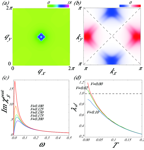
Figure 1: (Color online) Spin susceptibility $\mbox{Im}\,\chi_{s}(\mbox{\boldmath$q$},\omega)$ (a) and superconducting gap function $\mbox{Re}\,\phi(\mbox{\boldmath$k$},\omega=0)$ (b) are color-coded versus momentum for a bias $V=0.1$ above the critical value, with the doping level $\delta=0.14$, $U=4.5$, and $\mu=-0.35$. Dashed lines in (b) represent the nodes. (c) The peak value $\mbox{Im}\,\chi_{s}^{\rm peak}(\mbox{\boldmath$q$},\omega)$ versus $\omega$ for $V=0.1-0.2$ from top to bottom for $\mbox{\boldmath$q$}=(\pi,1.1\pi)$. $T=0.002$ for (a)-(c). (d) The temperature dependence of the Eliashberg eigenvalue $\lambda_{d}$ for the $d$-wave pairing for $V=0.0-0.1$ from top to bottom.

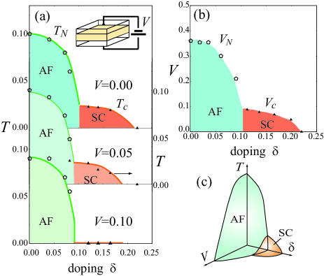
Figure 2: (Color online) (a) The phase diagrams for various values of the bias voltage $V$ with AF (antiferromagnetic) and SC (superconducting) phases with $U/t=4.5$. Origins of the three panels are shifted for clarity, and shadings representing different phases are only a guide to the eye. Inset: Schematic sample (shaded) configuration with two electrodes. (b) The zero-temperature phase diagram on the $(V,\delta)$ plane. (c) Schematic phase diagram in the $(T,V,\delta)$ space.

III Nonequilibrium phase transition

We have applied the above formalism to obtain the nonequilibrium phase diagram for the two-dimensional (square lattice) Hubbard model attached to two electrodes by numerically solving the equations self-consistently. In equilibrium the phase diagram within FLEX as obtained in Bickers et al. (1989) has an antiferromagnetic phase when the doping level $\delta=1-n$ is small, which is taken over by a $d$-wave superconductivity as $\delta$ is increased. So the interest is how the nonequilibrium situation modifies these. We first plot in Fig. 1(a) the spin susceptibility $\mbox{Im}\,\chi_{s}(\mbox{\boldmath$q$},\omega)$ for $V=0.1$ and a doping level $\delta=0.14$ The result shows that the antiferromagnetic fluctuation remains strong near half-filling, for which we have four incommensurate peaks around $\mbox{\boldmath$q$}=(\pi,\pi)$ in $k$-space, as in equilibrium. The effect of increased bias is that the peak height is reduced, and the peak position on energy axis shifts upwards as displayed in Fig. 1 (c), where $\mbox{Im}\,\chi_{s}^{\rm peak}(\mbox{\boldmath$q$},\omega)$ for $\mbox{\boldmath$q$}=(\pi,1.1\pi)$ is plotted. We notice that no features such as dip or hump appear around $\omega\sim V$. The dominant superconducting solution in Fig. 1(b) is again similar to the equilibrium case, that is, the $d$-wave gap has the largest $\lambda_{d}$ for the linearized Eliashberg equation. However, the critical temperature $T_{c}$ at which $\lambda_{d}$ reaches unity depends on $V$, as shown by the temperature dependence of $\lambda_{d}$ plotted in Fig. 1(d). So the bias $V$ reduces $T_{c}$, until finally the superconducting state no longer exists even at zero temperature when the bias becomes too strong. We define this as the critical bias $V_{c}$. For the region of the band filling for which the antiferromagnetic order dominates over the superconducting state, we can define the bias-dependent Néel temperature $T_{N}$ as the temperature at which the spin susceptibility divergesNeelDef . The spin susceptibility is reduced as the bias in increased, until the antiferromagnetic order vanishes even at zero temperature beyond the “critical Néel bias” $V_{N}$. The doping dependence of the Néel bias and the critical temperatures for a fixed bias is shown in Fig. 2 (a). We can see that, while the antiferromagnetic (AF) phase is relatively persistent, the superconducting (SC) region rapidly shrinks with the bias $V$ and disappears at $V\simeq 0.1$.

The phase diagram at zero-temperature is plotted on the $(V,\delta)$ plane in Fig. 2 (b). The Néel bias, peaked at the undoped point with $V_{N}\simeq 0.36$, decreases with the doping, and the AF phase is replaced with the SC phase around $\delta\simeq 0.1$ with a maximum critical bias for SC $V_{c}\simeq 0.1$. As we further increase the doping, the SC phase finally disappears. Figure 2 (c) schematically summarizes the phase transitions in the $(T,V,\delta)$ space.

IV Nonequilibrium distribution function

As was experimentally found in a tunneling measurement in a mesoscopic wire of copper by Pothier et al.,H. Pothier, S. Gueron,  Norman O. Birge, D. Esteve,  and M. H. Devoret (1997) the nonequilibrium electron distribution becomes smeared from the simple, double-step Fermi distribution $f_{\rm eff}^{0}$ due to electron scattering. In correlated materials with a strong electron-electron interaction, we expect a greater smearing effect to take place. Indeed, as we shall reveal below, the key feature to understand the nonequilibrium phase diagram for the open Hubbard model may be captured by the way in which the nonequilibrium distribution function is rounded by the interaction effect.

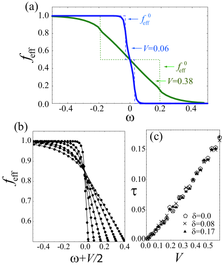
Figure 3: (Color online) (a) Nonequilibrium distribution function for two values of the bias, $V=0.06$ or $V=0.38$, at half filling ($\delta=0$). Dashed lines are the noninteracting distribution function $f_{\rm eff}^{0}$. (b) Nonequilibrium distribution function (dots) against $\omega$ in the $\omega<-V/2$ region for $V=0.08,\;0.19,\;0.32,\;0.47,\;0.63,\;0.80$ from the top, where curves represent a fit with eq.(30). (c) The smearing parameter $\tau$ against the bias $V$ for various values of $\delta$ and fixed $U=4.5$ and $T=0$. Fitting errors are smaller than the size of each symbol.

Figure 3 (a) plots the effective distribution $f_{\rm eff}$ defined in eq.(19) obtained self-consistently for two values of the bias $V$. The temperature in the electrodes, hence in $f_{\rm eff}^{0}$, is set to zero. If we compare the result with the corresponding noninteracting distribution function $f_{\rm eff}^{0}$ (eq.(20)) (dashed lines), $f_{\rm eff}$ is seen to significantly deviate from $f_{\rm eff}^{0}$. More importantly, we find here that the effective temperature approximation breaks down, that is, we cannot fit $f_{\rm eff}$ to $f_{\rm eff}^{0}$ with the temperature as a fitting parameter. Instead, the best fit to the data is given by

$$f_{\rm eff}^{\rm fit}=\left\{\begin{array}[]{cl}1-\alpha e^{(\omega+V/2)/\tau},&\omega<-V/2\\ -(1-2\alpha)\omega/V+1/2,&-V/2\leq\omega<V/2\\ \alpha e^{-(\omega-V/2)/\tau},&V/2\leq\omega\end{array}\right.$$ (30)

where $\alpha$ and $\tau$ are the fitting parameters. The parameter $\tau$ having the dimension of energy represents the extent to which the distribution is smeared from the double-step function. We have found in Fig. 3 (b) that the fitting function eq.(30) is adequate in the present open Hubbard model in that all the data for various values of the parameters ($V,\Gamma,U,\delta,\ldots$) are reproduced within the numerical errors. If we specifically plot the bias-dependence of the smearing parameter in Fig. 3 (c), we can see that they fall upon an universal curve. When $V$ is small, one can approximate this with a linear relation,

$$\tau\propto V.$$ (31)

The proportionality constant depends on the interaction strength $U$ and the coupling $\Gamma$ to the electrodes, but not on the filling $\delta$ as seen from the figure. The constant is reduced when the coupling to the electrode becomes stronger.

From the viewpoint of the smeared distribution, we can conceive the bias-driven phase transitions in the following way. We have seen in Fig. 2 (b) that the AF (SC) orders die out at $V\simeq 0.4$ ($V\simeq 0.1$) respectively. In terms of eq.(31), these values correspond to the smearing parameters $\tau\simeq 0.1$ ($\tau\simeq 0.02$). We can then note that these values are similar to the highest Néel (critical) temperatures in the zero bias phase diagram (Fig. 2 (a), upper panel). Thus, the transition takes place when the smearing parameter $\tau$ attains a value (depth of each phase in the phase diagram in Fig. 2 (c) as translated to $\tau$) that is similar to the transition temperature (height in the same phase diagram). AF spin fluctuations are suppressed in finite bias voltages in this manner, which is similar to what happens in itinerant electron magnets A. Mitra, S. Takei, Y. B. Kim, and A. J. Millis (2006).

V Discussion

We have obtained a nonequilibrium phase diagram for the two-dimensional Hubbard model, and pointed out the possibility of controlling the phases in strongly correlated heterostructures (i.e., electrode-system-electrode) by external bias. Both of AF and SC regions shrink with the bias $V$, which we attribute to the smearing of the nonequilibrium distribution function. While the smearing can be reduced if we make the system more strongly coupled to the electrodes (in e.g. a thinner sample), this will lead to the destruction of orders because a larger coupling $\Gamma$ to electrodes will make the spin fluctuations weaker. Thus we conclude the smearing of the distribution function is an important property characterizing correlated electron systems out of equilibrium, and an experimental verification of this should be interesting. We have to make a caution that FLEX employed here has limitations in that it ignores the vertex correction, and cannot address, due to its weak-coupling nature, the behavior close to the Mott insulator point, as mentioned. Effects of electrodes (on e.g. the pairing symmetry) when they are attached laterally are also intriguing. A more ambitious future problem is a possibility of bi-carrier induced superconductivity in nonequilibrium, for which the present formalism may serve as a starting point.

TO wishes to thank Thomas Dahm and Yoichi Yanase for helpful advices.

References

- Y. Tokura (2006) Y. Tokura, J. Phys. Soc. Jpn. 75, 011001 (2006).
- Y. Taguchi T. Matsumoto and Y. Tokura (2000) Y. Taguchi, T. Matsumoto, and Y. Tokura, Phys. Rev. B 62, 7015 (2000).
- T. Oka R. Arita and H. Aoki (2003) T. Oka, R. Arita, and H. Aoki, Phys. Rev. Lett. 91, 066406 (2003).
- A. Mitra, S. Takei, Y. B. Kim, and A. J. Millis (2006) A. Mitra, S. Takei, Y. B. Kim, and A. J. Millis, Phys. Rev. Lett. 97, 236808 (2006).
- A. Ohtomo and H. Y. Hwang (2004) A. Ohtomo and H. Y. Hwang, Nature 427, 423 (2004).
- N. Reyren et al. (2007) N. Reyren et al., Science 317, 1196 (2007).
- K. Ueno et al. (2008) K. Ueno et al., Nature Material 7, 855 (2008).
- S. Okamoto and A. J. Millis (2004) S. Okamoto and A. J. Millis, Nature 428, 630 (2004).
- T. Oka and N. Nagaosa (2005) T. Oka and N. Nagaosa , Phys. Rev. Lett. 95, 266403 (2005).
- S. Okamoto (2008) S. Okamoto, Phy. Rev. Lett. 101, 116807 (2008).
- H. Pothier, S. Gueron, Norman O. Birge, D. Esteve, and M. H. Devoret (1997) H. Pothier, S. Gueron, N. O. Birge, D. Esteve, and M. H. Devoret, Phys. Rev. Lett. 79, 3490 (1997).
- Bickers et al. (1989) N. E. Bickers, D. J. Scalapino, and S. R. White, Phys. Rev. Lett. 62, 961 (1989).
- Bickers and White (1991) N. E. Bickers and S. R. White, Phys. Rev. B 43, 8044 (1991).
- J. J. Chang and D. J. Scalapino (1978) J. J. Chang and D. J. Scalapino, J. Low Temp. 31, 1 (1978).
- A. F. G. Wyatt, V. M. Dmitriev, V. S. Moore, and F. W. Sheard (1966) A. F. G. Wyatt et al, , Phys. Rev. Lett. 16, 1166 (1966).
- T. Kommers and J. Clarke (1977) T. Kommers and J. Clarke, Phys. Rev. Lett. 38, 1091 (1977).
- D. Dalidovich and P. Phillips (2004) D. Dalidovich and P. Phillips, Phys. Rev. Lett. 93, 027004 (2004).
- Mitra (2008) A. Mitra, Phys. Rev. B 78, 214512 (2008).
- Takei and Kim (2008) S. Takei and Y. B. Kim, Phys.l Rev. B 78, 165401 (2008).
- M. Imada, A. Fujimori, and Y. Tokura (1998) M. Imada, A. Fujimori, and Y. Tokura, Rev. Mod. Phys. 70, 1039 (1998).
- Pao and Bickers (1994) C.-H. Pao and N. E. Bickers, Phys. Rev. Lett. 72, 1870 (1994).
- Monthoux and Scalapino (1994) P. Monthoux and D. J. Scalapino, Phys. Rev. Lett. 72, 1874 (1994).
- Dahm and Tewordt (1995a) T. Dahm and L. Tewordt, Phys. Rev. Lett. 74, 793 (1995a).
- Millis et al. (1990) A. J. Millis, H. Monien, and D. Pines, Phys. Rev. B 42, 167 (1990).
- Monthoux et al. (1991) P. Monthoux, A. V. Balatsky, and D. Pines, Phys. Rev. Lett. 67, 3448 (1991).
- (26) K. Kuroki and H. Aoki, Phys. Rev. Lett. 76, 4400 (1996); Phys. Rev. B 56, R14287 (1997).
- Werner et al. (2009) P. Werner, T. Oka, and A. J. Millis, Phys. Rev. B 79, 035320 (2009).
- J. Rammer (2007) J. Rammer, Quantum Field Theory of Non-equilibrium States (Cambridge Univ. Press, 2007).
- A. P. Jauho, N. S. Wingreen and Y. Meir (1994) A. P. Jauho, N. S. Wingreen, and Y. Meir, Phys. Rev. B 50, 5528 (1994).
- (30) See for example, N. Tsuji, T. Oka, and H. Aoki, Phys. Rev. Lett. 103, 047403 (2009).
- Dahm and Tewordt (1995b) T. Dahm and L. Tewordt, Phys. Rev. B 52, 1297 (1995b).
- (32) In numerical calculations the divergence is rounded, and we adopt an often employed criterion for the transition, Max[.