Classical and Thermodynamic work fluctuations

Mamata Sahoo    A.M Jayannavar Institute of Physics,  Sachivalaya Marg,   Bhubaneswar-751005, India
Abstract

Abstract:  We have studied the nature of classical work (Wcsubscript𝑊𝑐W_{c}) and thermodynamic work (W𝑊W) fluctuations in systems driven out of equilibrium both in transient and time periodic steady state. As the observation time of trajectory increases, we show that the number of trajectories which exhibit excursions away from the typical behaviour i.e., Wc<0subscript𝑊𝑐0W_{c}<0, W<ΔF𝑊Δ𝐹W<\Delta F and dissipated heat Q<0𝑄0Q<0 decreases as anticipated for macroscopic time scales. Analytical expressions for such trajectories are obtained. Trajectory for which Wc<0subscript𝑊𝑐0W_{c}<0 may not correspond to W<ΔF𝑊Δ𝐹W<\Delta F or Q<0𝑄0Q<0. The applicability of steady state fluctuation theorems are discussed in our linear as well as nonlinear models.

Key Words: Fluctuation phenomena, classical work and thermodynamic work
PACS numbers: 05.40.-a, 05.70.Ln, 05.40.Jc

Corresponding Author: A.M. Jayannavar
Email address : jayan@iopb.res.in

I Introduction

Over last decade, nonequilibrium fluctuation theorems have attracted much interest. They provide relations for physical quantities such as work, heat and entropy in driven nonequilibrium systems, independent of the nature of driving [1-17]. The fluctuation relations are statements about the symmetry of the distributions of the physical quantities around zero and not around the maximum. These distribution functions exhibit finite weight for negative values for physical quantities of interest, which are usually rare and are related to transient second law violating contributions at microscopic length scales. Fluctuation theorems quantify the probability of those non-equilibrium trajectories, taken individually, violate some of the inequalities of the thermodynamics. For average quantities, these theorems lead to inequalities consistent with the second law of thermodynamics. In our present study, we are mainly concerned with Jarzynski Equality (JE) [10,11] for thermodynamic work (W𝑊W) and Bochkov-Kuzovlev identity (BKI) for classical work (Wcsubscript𝑊𝑐W_{c})[14-17]. JE relates the nonequilibrium work done with equilibrium free energy difference (ΔF=FBFAΔ𝐹subscript𝐹𝐵subscript𝐹𝐴\Delta F=F_{B}-F_{A}) between two thermodynamic states. These two thermodynamic states are uniquely characterized by the initial (A) and final (B) values of the time dependent protocol. JE is given by

eβW=eβΔF,delimited-⟨⟩superscript𝑒𝛽𝑊superscript𝑒𝛽Δ𝐹\langle e^{-\beta W}\rangle=e^{-\beta\Delta F}, (1)

where W𝑊W is the thermodynamic work. The angular bracket delimited-⟨⟩\langle\cdots\rangle denotes the average over an ensemble of realizations, starting from initial equilibrium configurations. W𝑊W is defined as W=0τU(x,t)t𝑑t𝑊superscriptsubscript0𝜏𝑈𝑥𝑡𝑡differential-d𝑡W=\int_{0}^{\tau}\frac{\partial U(x,t)}{\partial t}dt, where U(x,t)𝑈𝑥𝑡U(x,t) is the effective potential of the system. Incidentally, the JE finds its counterpart in the relation known as Bochkov-Kuzovlev identity which has been proposed much earlier [14-17]

eβWc=1delimited-⟨⟩superscript𝑒𝛽subscript𝑊𝑐1\langle e^{-\beta W_{c}}\rangle=1 (2)

where Wcsubscript𝑊𝑐W_{c} is the classical work. If the potential is decomposed as U(x,t)=U0(x)+Up(x,t)𝑈𝑥𝑡subscript𝑈0𝑥subscript𝑈𝑝𝑥𝑡U(x,t)=U_{0}(x)+U_{p}(x,t), the classical work done over a time interval τ𝜏\tau is defined as Wc=0τUp(x,t)xx˙𝑑tsubscript𝑊𝑐superscriptsubscript0𝜏subscript𝑈𝑝𝑥𝑡𝑥˙𝑥differential-d𝑡W_{c}=-\int_{0}^{\tau}\frac{\partial U_{p}(x,t)}{\partial x}\dot{x}dt.   For the validity of BKI,  the initial equilibrium distribution must correspond to the time independent potential (Pe(x0)=NeU0(x0)kBTsubscript𝑃𝑒subscript𝑥0𝑁superscript𝑒subscript𝑈0subscript𝑥0subscript𝑘𝐵𝑇P_{e}(x_{0})=Ne^{-\frac{U_{0}(x_{0})}{k_{B}T}}, N𝑁N being the normalization constant). Seifert has shown that both JE and BKI are special cases of more general result, obtained within a framework that defines entropy production in nonequilibrium state [18,19]. When the internal energy of the system is defined by the bare Hamiltonian/potential, then classical work is defined as the work performed by the application of an external force that affects the system in a fixed landscape of the bare Hamiltonian. To define thermodynamic work, external time dependent perturbation is treated as the time dependent contribution to the internal energy of the system [20]. The work done by the system on the external bodies which produce a change in the Hamiltonian is known as thermodynamic work W𝑊W. It turns out that W𝑊W is more useful than Wcsubscript𝑊𝑐W_{c} for the reconstruction of free energy landscapes. Using Jensen’s inequality, from eqns. (1) and (2) it follows that WΔFdelimited-⟨⟩𝑊Δ𝐹\langle W\rangle\geq\Delta F, Wc0delimited-⟨⟩subscript𝑊𝑐0\langle W_{c}\rangle\geq 0, which are consistent with the physics at macroscopic scales. Observations of realizations wherein W<ΔF𝑊Δ𝐹W<\Delta F or Wc<0subscript𝑊𝑐0W_{c}<0 are treated as excursions away from the typical macroscopic behaviour. The finite time trajectories for which W<ΔF𝑊Δ𝐹W<\Delta F, are sometimes referred to as transient second law violating trajectories [21]. In our work, we have also studied decrease in the number of such trajectories as a function of time of observations and some pertinent questions are raised. Nature of the fluctuations in W𝑊W and Wcsubscript𝑊𝑐W_{c} are studied in a nonlinear system exhibiting stochastic resonance(SR) [22-29]. Finally we have analyzed the validity of SSFT for W𝑊W and Wcsubscript𝑊𝑐W_{c}.

II Driven linear systems

II.1 Model

We consider a linear model, i.e.,  a overdamped Brownian particle in a one dimensional harmonic potential U0(x)=12kx2subscript𝑈0𝑥12𝑘superscript𝑥2U_{0}(x)=\frac{1}{2}kx^{2} in the presence of an external time dependent potential Up=Ax(t)sin(ωt+ϕ)subscript𝑈𝑝𝐴𝑥𝑡𝜔𝑡italic-ϕU_{p}=-Ax(t)\sin(\omega t+\phi), where A𝐴A , ω𝜔\omega are the amplitude, frequency of the external drive respectively and ϕitalic-ϕ\phi is an initial phase. The dynamics of the particle is described by the Langevin’s equation [30]

γdxdt=U(x,t)x+ξ(t),𝛾𝑑𝑥𝑑𝑡𝑈𝑥𝑡𝑥𝜉𝑡\gamma\frac{dx}{dt}=-\frac{\partial U(x,t)}{\partial x}+\xi(t), (3)

where U(x,t)=U0(x)+Up(x,t)𝑈𝑥𝑡subscript𝑈0𝑥subscript𝑈𝑝𝑥𝑡U(x,t)=U_{0}(x)+U_{p}(x,t).  The random force field ξ(t)𝜉𝑡\xi(t) is a zero mean Gaussian white noise, i.e., ξ(t)ξ(t)=2Dδ(tt)delimited-⟨⟩𝜉𝑡𝜉superscript𝑡2𝐷𝛿𝑡superscript𝑡\langle\xi(t)\xi(t^{{}^{\prime}})\rangle=2D\delta(t-t^{{}^{\prime}}), D=γkBT𝐷𝛾subscript𝑘𝐵𝑇D=\gamma k_{B}T is the noise strength of the medium. Here γ𝛾\gamma is the friction coefficient, kBsubscript𝑘𝐵k_{B} is the Boltzmann constant and T𝑇T is the absolute temperature of the bath. In the following we use a dimensionless form of eqn.(3),  namely

dxdt=U(x,t)x+ξ(t),𝑑𝑥𝑑𝑡𝑈𝑥𝑡𝑥𝜉𝑡\frac{dx}{dt}=-\frac{\partial U(x,t)}{\partial x}+\xi(t), (4)

All the calculated quantities are in dimensionless form.

II.2 Thermodynamic work distributions:

Thermodynamic work(W𝑊W) done on the system by the external drive over a time t𝑡t is given

W=Aω0tx(t)cos(ωt+ϕ)𝑑t.𝑊𝐴𝜔superscriptsubscript0𝑡𝑥superscript𝑡𝜔superscript𝑡italic-ϕdifferential-dsuperscript𝑡W=-A\omega\int_{0}^{t}x(t^{{}^{\prime}})\cos(\omega t^{{}^{\prime}}+\phi)dt^{{}^{\prime}}. (5)

The formal solution of eqn.(4) is

x(t)=x0exp(kt)+0t𝑑texp(k(tt))[Asin(ωt+ϕ)+ξ(t)].𝑥𝑡subscript𝑥0𝑘𝑡superscriptsubscript0𝑡differential-dsuperscript𝑡𝑘𝑡superscript𝑡delimited-[]𝐴𝜔superscript𝑡italic-ϕ𝜉superscript𝑡x(t)=x_{0}\exp(-kt)+\int_{0}^{t}dt^{{}^{\prime}}\exp(-k(t-t^{{}^{\prime}}))[A\sin(\omega t^{{}^{\prime}}+\phi)+\xi(t^{{}^{\prime}})]. (6)

Where x0subscript𝑥0x_{0} is the initial coordinate of the particle. The initial distribution for x0subscript𝑥0x_{0} is assumed to be the equilibrium canonical distribution, Pe(x0)=kβ2πexp(kβ2(x0Aksin(ϕ))2)subscript𝑃𝑒subscript𝑥0𝑘𝛽2𝜋𝑘𝛽2superscriptsubscript𝑥0𝐴𝑘italic-ϕ2P_{e}(x_{0})=\sqrt{\frac{k\beta}{2\pi}}\exp(-\frac{k\beta}{2}(x_{0}-\frac{A}{k}\sin(\phi))^{2}). From eqns.(5) and (6), it follows that thermodynamic work done is a linear functional of the Gaussian variable ξ(t)𝜉𝑡\xi(t) . Hence the distribution P(W)𝑃𝑊P(W) of work W𝑊W is a Gaussian [31-33]. By a simple algebra one can evaluate P(W)𝑃𝑊P(W) analytically. The full probability distribution P(W)𝑃𝑊P(W) is given by

P(W)=12πσ2exp[(WW)22σ2]𝑃𝑊12𝜋superscript𝜎2superscript𝑊delimited-⟨⟩𝑊22superscript𝜎2\displaystyle P(W)=\frac{1}{\sqrt{2\pi\sigma^{2}}}\exp{\left[-\frac{(W-\langle W\rangle)^{2}}{2\sigma^{2}}\right]} (7)

where the analytical expressions for the mean thermodynamic work done(Wdelimited-⟨⟩𝑊\langle W\rangle) is given in Appendix-A. The variance σ2=W2W2superscript𝜎2delimited-⟨⟩superscript𝑊2superscriptdelimited-⟨⟩𝑊2\sigma^{2}=\langle W^{2}\rangle-\langle W\rangle^{2} is given by

W2W2delimited-⟨⟩superscript𝑊2superscriptdelimited-⟨⟩𝑊2\displaystyle\langle W^{2}\rangle-\langle W\rangle^{2} =\displaystyle= 2βW+A2kβsin2(ωt+ϕ).2𝛽delimited-⟨⟩𝑊superscript𝐴2𝑘𝛽superscript2𝜔𝑡italic-ϕ\displaystyle\frac{2}{\beta}\langle W\rangle+\frac{A^{2}}{k\beta}\sin^{2}(\omega t+\phi). (8)

The thermodynamic work done over a time interval τ𝜏\tau satisfies JE,

eβW=eβΔFdelimited-⟨⟩superscript𝑒𝛽𝑊superscript𝑒𝛽Δ𝐹\displaystyle\langle e^{-\beta W}\rangle=e^{-\beta\Delta F} (9)

where ΔF=A22ksin2(ωτ+ϕ)Δ𝐹superscript𝐴22𝑘superscript2𝜔𝜏italic-ϕ\Delta F=-\frac{A^{2}}{2k}\sin^{2}(\omega\tau+\phi),  is the free energy difference between two thermodynamic states with potentials U(x0)=12kx02Ax0sin(ϕ)𝑈subscript𝑥012𝑘superscriptsubscript𝑥02𝐴subscript𝑥0italic-ϕU(x_{0})=\frac{1}{2}kx_{0}^{2}-Ax_{0}\sin(\phi) and U(x,τ)=12kx2Ax(τ)sin(ωτ+ϕ)𝑈𝑥𝜏12𝑘superscript𝑥2𝐴𝑥𝜏𝜔𝜏italic-ϕU(x,\tau)=\frac{1}{2}kx^{2}-Ax(\tau)\sin(\omega\tau+\phi) respectively .

We furthur study the statistics of the thermodynamic work done, W𝑊W, in the time asymptotic regime (i.e, in the limit t𝑡t\rightarrow\infty). In this limit, probability distributions are time periodic with a period of magnitude 2πω2𝜋𝜔\frac{2\pi}{\omega}.  The average work done(Wτdelimited-⟨⟩subscript𝑊𝜏\langle W_{\tau}\rangle) over a time of observation τ𝜏\tau in the time periodic steady state is

Wτdelimited-⟨⟩subscript𝑊𝜏\displaystyle\langle W_{\tau}\rangle =\displaystyle= limt[W(t+τ)W(t)]subscript𝑡delimited-[]delimited-⟨⟩𝑊𝑡𝜏delimited-⟨⟩𝑊𝑡\displaystyle\lim_{t\rightarrow\infty}[\langle W(t+\tau)\rangle-\langle W(t)\rangle] (10)
=\displaystyle= A2ω2τ2(k2+ω2).superscript𝐴2superscript𝜔2𝜏2superscript𝑘2superscript𝜔2\displaystyle\frac{A^{2}\omega^{2}\tau}{2(k^{2}+\omega^{2})}.

The variance(στ2superscriptsubscript𝜎𝜏2\sigma_{\tau}^{2}) of Wτsubscript𝑊𝜏W_{\tau} averaged over a time of observation τ𝜏\tau is given by

στ2superscriptsubscript𝜎𝜏2\displaystyle\sigma_{\tau}^{2} =\displaystyle= Wτ2Wτ2delimited-⟨⟩superscriptsubscript𝑊𝜏2superscriptdelimited-⟨⟩subscript𝑊𝜏2\displaystyle\langle W_{\tau}^{2}\rangle-\langle W_{\tau}\rangle^{2} (11)
=\displaystyle= 2βWτ+Δ(τ)2𝛽delimited-⟨⟩subscript𝑊𝜏Δ𝜏\displaystyle\frac{2}{\beta}\langle W_{\tau}\rangle+\Delta(\tau)

The analytical expression for Δ(τ)Δ𝜏\Delta(\tau) is given in Appendix-C. The distribution for Wτsubscript𝑊𝜏W_{\tau} is Gaussian. However, it does not satisfy the fluctuation dissipation relation, namely στ2=2βWτsuperscriptsubscript𝜎𝜏22𝛽delimited-⟨⟩subscript𝑊𝜏\sigma_{\tau}^{2}=\frac{2}{\beta}\langle W_{\tau}\rangle [4]. Hence SSFT is not valid over small time of observation. However, Wτdelimited-⟨⟩subscript𝑊𝜏\langle W_{\tau}\rangle is an extensive quantity in τ𝜏\tau, whereas Δ(τ)Δ𝜏\Delta(\tau) saturates to a finite value for τ1kmuch-greater-than𝜏1𝑘\tau\gg\frac{1}{k}. For large τ𝜏\tau, 2βWτΔ(τ)much-greater-than2𝛽delimited-⟨⟩subscript𝑊𝜏Δ𝜏\frac{2}{\beta}\langle W_{\tau}\rangle\gg\Delta(\tau) and the contribution of Δ(τ)Δ𝜏\Delta(\tau) to the variance στ2superscriptsubscript𝜎𝜏2\sigma_{\tau}^{2} can be ignored in eqn.(11). Under this approximation SSFT holds. Here SSFT implies

P(Wτ)P(Wτ)=eβWτ𝑃subscript𝑊𝜏𝑃subscript𝑊𝜏superscript𝑒𝛽subscript𝑊𝜏\displaystyle\frac{P(W_{\tau})}{P(-W_{\tau})}=e^{\beta W_{\tau}} (12)

II.3 Classical work distributions:

Classical work (Wcsubscript𝑊𝑐W_{c}) done on the system by the external drive Asin(ωt+ϕ)𝐴𝜔𝑡italic-ϕA\sin(\omega t+\phi) over a duration of time t𝑡t is given by [14,15]

Wcsubscript𝑊𝑐\displaystyle W_{c} =\displaystyle= 0tAsin(ωt+ϕ)x˙(t)𝑑tsuperscriptsubscript0𝑡𝐴𝜔superscript𝑡italic-ϕ˙𝑥superscript𝑡differential-dsuperscript𝑡\displaystyle\int_{0}^{t}A\sin(\omega t^{{}^{\prime}}+\phi)\dot{x}(t^{{}^{\prime}})dt^{{}^{\prime}} (13)
=\displaystyle= W+[Asin(ωt+ϕ)x(t)Asin(ϕ)x(0)]𝑊delimited-[]𝐴𝜔𝑡italic-ϕ𝑥𝑡𝐴italic-ϕ𝑥0\displaystyle W+\left[A\sin(\omega t+\phi)x(t)-A\sin(\phi)x(0)\right]

Note that classical work (Wcsubscript𝑊𝑐W_{c}) differs from the thermodynamic work(W𝑊W) by a boundary term.  From eqns.(13) and (6) it follows that Wcsubscript𝑊𝑐W_{c} is a linear functional of a Gaussian variable ξ(t)𝜉𝑡\xi(t),  consequently P(Wc)𝑃subscript𝑊𝑐P(W_{c}) is a Gaussian and is given by

P(Wc)=12πσc2exp[(WcWc)22σc2]𝑃subscript𝑊𝑐12𝜋superscriptsubscript𝜎𝑐2superscriptsubscript𝑊𝑐delimited-⟨⟩subscript𝑊𝑐22superscriptsubscript𝜎𝑐2\displaystyle P(W_{c})=\frac{1}{\sqrt{2\pi\sigma_{c}^{2}}}\exp\left[-\frac{(W_{c}-\langle W_{c}\rangle)^{2}}{2\sigma_{c}^{2}}\right] (14)

where Wcdelimited-⟨⟩subscript𝑊𝑐\langle W_{c}\rangle is the mean classical work done over a time interval t𝑡t and σc2superscriptsubscript𝜎𝑐2\sigma_{c}^{2} is the fluctuation or variance of Wcsubscript𝑊𝑐W_{c}.   These quantities can be evaluated analytically. The expression for average or mean classical work(Wcdelimited-⟨⟩subscript𝑊𝑐\langle W_{c}\rangle) is given in Appendix-B.

The variance in classical work (σc2superscriptsubscript𝜎𝑐2\sigma_{c}^{2}) over a transient time t𝑡t is given by

σc2superscriptsubscript𝜎𝑐2\displaystyle\sigma_{c}^{2} =\displaystyle= Wc2Wc2delimited-⟨⟩superscriptsubscript𝑊𝑐2superscriptdelimited-⟨⟩subscript𝑊𝑐2\displaystyle\langle W_{c}^{2}\rangle-\langle W_{c}\rangle^{2} (15)
=\displaystyle= 2βWc2𝛽delimited-⟨⟩subscript𝑊𝑐\displaystyle\frac{2}{\beta}\langle W_{c}\rangle

To calculate Wcsubscript𝑊𝑐W_{c} and σc2superscriptsubscript𝜎𝑐2\sigma_{c}^{2},  we assumed initially the system to be in equilibrium with distribution Pe(x0)=(kβ2π)eβkx022P_{e}(x_{0})=\sqrt{(}\frac{k\beta}{2\pi})e^{-\beta\frac{kx_{0}^{2}}{2}}. The expression for P(Wc)𝑃subscript𝑊𝑐P(W_{c}) is consistent with BKI.

eβWc=1.delimited-⟨⟩superscript𝑒𝛽subscript𝑊𝑐1\langle e^{-\beta W_{c}}\rangle=1. (16)

The average classical work (Wcτdelimited-⟨⟩subscript𝑊𝑐𝜏\langle W_{c\tau}\rangle) done over a time of observation τ𝜏\tau in the time periodic steady state, is given by

Wcτ=A2ω2τ2(k2+ω2),delimited-⟨⟩subscript𝑊𝑐𝜏superscript𝐴2superscript𝜔2𝜏2superscript𝑘2superscript𝜔2\displaystyle\langle W_{c\tau}\rangle=\frac{A^{2}\omega^{2}\tau}{2(k^{2}+\omega^{2})}, (17)

which has the same magnitude as that of Wτdelimited-⟨⟩subscript𝑊𝜏\langle W_{\tau}\rangle and is independent of ϕitalic-ϕ\phi. The distribution P(Wcτ)𝑃subscript𝑊𝑐𝜏P(W_{c\tau}) is Gaussian. The variance (σcτ)\sigma_{c\tau)}) is given by

σcτ=2βWcτ+Δ1(τ)subscript𝜎𝑐𝜏2𝛽delimited-⟨⟩subscript𝑊𝑐𝜏subscriptΔ1𝜏\displaystyle\sigma_{c\tau}=\frac{2}{\beta}\langle W_{c\tau}\rangle+\Delta_{1}(\tau) (18)

An expression for Δ1(τ)subscriptΔ1𝜏\Delta_{1}(\tau) is given in Appendix-D. For τ1kmuch-greater-than𝜏1𝑘\tau\gg\frac{1}{k}, Δ1(τ)subscriptΔ1𝜏\Delta_{1}(\tau) saturates to a finite value. For large τ𝜏\tau, for which 2βWcτΔ1(τ)much-greater-than2𝛽delimited-⟨⟩subscript𝑊𝑐𝜏subscriptΔ1𝜏\frac{2}{\beta}\langle W_{c\tau}\rangle\gg\Delta_{1}(\tau) one can ignore Δ1(τ)subscriptΔ1𝜏\Delta_{1}(\tau) in eqn.(18). Under this condition the classical work satisfies SSFT.
Refer to caption
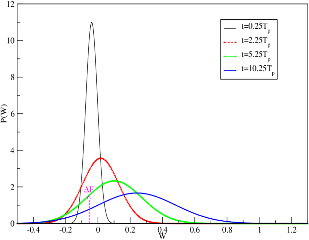
Figure 1: The distribution P(W)𝑃𝑊P(W) as a function of transient time t𝑡t (in units of Tpsubscript𝑇𝑝T_{p}) for parameters A=0.3𝐴0.3A=0.3, D=0.1𝐷0.1D=0.1, ω=0.1𝜔0.1\omega=0.1 and Tp=2πωsubscript𝑇𝑝2𝜋𝜔T_{p}=\frac{2\pi}{\omega}.

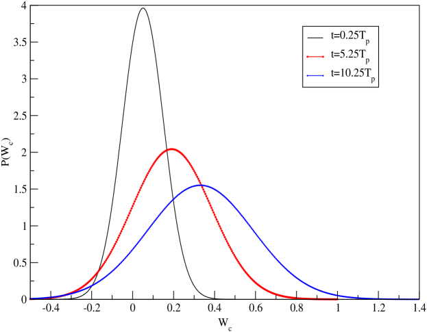
In fig(1) and (2), we have plotted the probability distributions of W𝑊W and Wcsubscript𝑊𝑐W_{c} for various values of time periods in the transient regime using our analytical results (eqns.(7),(14)). Other parameters are given in figure captions. For short time t=0.25Tp𝑡0.25subscript𝑇𝑝t=0.25T_{p} (Tpsubscript𝑇𝑝T_{p} being the time period of magnitude 2πω2𝜋𝜔\frac{2\pi}{\omega}), we notice that most of the weight of W𝑊W is located in the negative side. The weight towards negative side for values W<ΔF𝑊Δ𝐹W<\Delta F comes from the so called transient second law violating trajectories [21]. As we increase the time of observations, the total weight for W<ΔF𝑊Δ𝐹W<\Delta F (i.e., area under the curve P(W)𝑃𝑊P(W) between W=𝑊W=-\infty and W=ΔF𝑊Δ𝐹W=\Delta F) decreases (see fig(1)). We would like to emphasize that depending on the protocol and potential, one may obtain peak in P(W)𝑃𝑊P(W) at values W<ΔF𝑊Δ𝐹W<\Delta F, i.e., most probable value of W𝑊W is inconsistent with the classical macroscopic or thermodynamic results. However, W>ΔFdelimited-⟨⟩𝑊Δ𝐹\langle W\rangle>\Delta F is always satisfied. In contrast, Wcsubscript𝑊𝑐W_{c} does not exhibit a peak in the negative region. We have checked this separately for different systems for different protocols.
Refer to caption
Figure 2: The distribution P(Wc)𝑃subscript𝑊𝑐P(W_{c}) as a function of transient time t𝑡t (in units of Tpsubscript𝑇𝑝T_{p}) for parameters A=0.3𝐴0.3A=0.3, D=0.1𝐷0.1D=0.1, ω=0.1𝜔0.1\omega=0.1 and Tp=2πωsubscript𝑇𝑝2𝜋𝜔T_{p}=\frac{2\pi}{\omega}.

The physical quantities such as work (W𝑊W), heat (Q𝑄Q), total entropy (ΔStotΔsubscript𝑆𝑡𝑜𝑡\Delta S_{tot}) and internal energy (ΔUΔ𝑈\Delta U) can be calculated using the method of stochastic energetics [34]. For details, we refer to [26,27,28,35].
Refer to caption
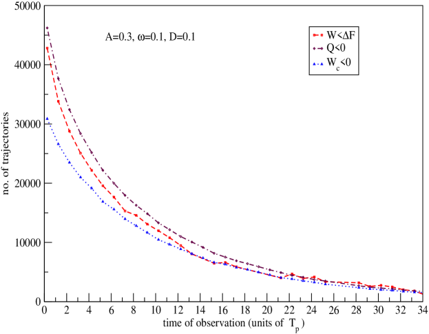
Figure 3: Number of trajectories for W<0𝑊0W<0, Q<0𝑄0Q<0 and Wcl<0subscript𝑊𝑐𝑙0W_{cl}<0 as a function of time t𝑡t (in units of Tpsubscript𝑇𝑝T_{p}). The physical parameters are same as in fig(1) and (2).

In fig(3) we have plotted number of trajectories which do not satisfy our conventional wisdom at macroscopic scale, namely W<ΔF𝑊Δ𝐹W<\Delta F, Wc<0subscript𝑊𝑐0W_{c}<0 and heat dissipated, Q<0𝑄0Q<0. For each individual trajectory, W𝑊W, Wcsubscript𝑊𝑐W_{c} and Q𝑄Q are calculated. In our simulation, we have generated 105superscript10510^{5} trajectories. Number of trajectories for which Wc<0subscript𝑊𝑐0W_{c}<0, W<ΔF𝑊Δ𝐹W<\Delta F and Q<0𝑄0Q<0 are all different. Trajectory for which Wc<0subscript𝑊𝑐0W_{c}<0 need not correspond to W<ΔF𝑊Δ𝐹W<\Delta F or Q<0𝑄0Q<0. It can be readily shown that if N𝑁N is the total number of observed trajectories for Wcsubscript𝑊𝑐W_{c}, then the number of trajectories Nsuperscript𝑁N^{{}^{\prime}} for which Wc<0subscript𝑊𝑐0W_{c}<0 are given by N=N2Erfc(Wc2σWc2)superscript𝑁𝑁2Erfcdelimited-⟨⟩subscript𝑊𝑐2superscriptsubscript𝜎subscript𝑊𝑐2N^{{}^{\prime}}=\frac{N}{2}\textrm{Erfc}(\frac{\langle W_{c}\rangle}{\sqrt{2\sigma_{W_{c}}^{2}}}). In the time asymptotic regime Wcdelimited-⟨⟩subscript𝑊𝑐\langle W_{c}\rangle scales with t𝑡t and the decay of Nsuperscript𝑁N^{{}^{\prime}} with time t𝑡t is given by N=atexp(ct)superscript𝑁𝑎𝑡𝑐𝑡N^{{}^{\prime}}=\frac{a}{\sqrt{t}}\exp(-ct), where a𝑎a and c𝑐c are constants. For our present problem a=2D(k2+γ2ω2)A2γω2π𝑎2𝐷superscript𝑘2superscript𝛾2superscript𝜔2superscript𝐴2𝛾superscript𝜔2𝜋a=\sqrt{\frac{2D(k^{2}+\gamma^{2}\omega^{2})}{A^{2}\gamma\omega^{2}\pi}} and c=A2γω28D(k2+γ2ω2)𝑐superscript𝐴2𝛾superscript𝜔28𝐷superscript𝑘2superscript𝛾2superscript𝜔2c=\frac{A^{2}\gamma\omega^{2}}{8D(k^{2}+\gamma^{2}\omega^{2})}. The number of trajectories for which W<ΔF𝑊Δ𝐹W<\Delta F in the large time limit, decay with the same functional form as that for Wc<0subscript𝑊𝑐0W_{c}<0. Hence there is no correlation amongst trajectories in regard to the transient violations in W𝑊W, Wcsubscript𝑊𝑐W_{c} and Q𝑄Q. For our simple linear problem and protocol (up to time periods 12absent12\approx 12), number of trajectories for which Q<0𝑄0Q<0 are greater than W<ΔF𝑊Δ𝐹W<\Delta F which in turn are greater than Wc<0subscript𝑊𝑐0W_{c}<0. This is not a general rule. Depending on the system and protocol, different possibilities exist. However, one common observation is that the number of trajectories which defy our general classical notion for W𝑊W, Wcsubscript𝑊𝑐W_{c} and Q𝑄Q decrease monotonically as time of observation is increased, leading to classical thermodynamic behaviour in the time asymptotic regime as is evident from fig(3).
Refer to caption
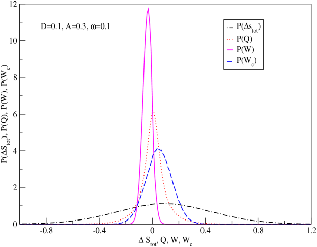
Figure 4: The distributions P(ΔStot)𝑃Δsubscript𝑆𝑡𝑜𝑡P(\Delta S_{tot}), P(W)𝑃𝑊P(W), P(Wc)𝑃subscript𝑊𝑐P(W_{c}) and P(Q)𝑃𝑄P(Q) for the parameters A=0.3𝐴0.3A=0.3, D=0.1𝐷0.1D=0.1, ω=0.1𝜔0.1\omega=0.1 and for t=Tp4𝑡subscript𝑇𝑝4t=\frac{T_{p}}{4}.

To put the probability distributions of physical quantities W𝑊W, Wcsubscript𝑊𝑐W_{c}, Q𝑄Q and ΔStotΔsubscript𝑆𝑡𝑜𝑡\Delta S_{tot} in the same perspective we have generated 105superscript10510^{5} trajectories of Brownian particle. Total entropy production ΔStotΔsubscript𝑆𝑡𝑜𝑡\Delta S_{tot} comprises of two parts namely system entropy and medium entropy. For details we refer to [18,19]. For each stochastic trajectory we calculate W𝑊W, Wcsubscript𝑊𝑐W_{c}, Q𝑄Q and ΔStotΔsubscript𝑆𝑡𝑜𝑡\Delta S_{tot} and using these values, the obtained P(W)𝑃𝑊P(W), P(Wc)𝑃subscript𝑊𝑐P(W_{c}), P(Q)𝑃𝑄P(Q) and P(ΔStot)𝑃Δsubscript𝑆𝑡𝑜𝑡P(\Delta S_{tot}) are plotted in fig (4). Areas under the curves for W<ΔF𝑊Δ𝐹W<\Delta F, Wc<0subscript𝑊𝑐0W_{c}<0, Q<0𝑄0Q<0 and ΔStot<0Δsubscript𝑆𝑡𝑜𝑡0\Delta S_{tot}<0 are different. In our linear problem the distribution for P(W)𝑃𝑊P(W), P(Wc)𝑃subscript𝑊𝑐P(W_{c}) and P(ΔStot)𝑃Δsubscript𝑆𝑡𝑜𝑡P(\Delta S_{tot}) are Gaussian, while that for P(Q)𝑃𝑄P(Q) is non Gaussian. It may be noted that by appropriately choosing the system and protocol most probable value of P(ΔStot)𝑃Δsubscript𝑆𝑡𝑜𝑡P(\Delta S_{tot}) can be shifted to the negative side, yet ΔStot>0delimited-⟨⟩Δsubscript𝑆𝑡𝑜𝑡0\langle\Delta S_{tot}\rangle>0. However, peak in P(Q)𝑃𝑄P(Q) corresponding to the most probable value occurs at positive values of Q𝑄Q only. Similar behaviour in regard to P(W)𝑃𝑊P(W) and P(Wc)𝑃subscript𝑊𝑐P(W_{c}) are pointed earlier. In the next section, we study the nature of fluctuations in W𝑊W and Wcsubscript𝑊𝑐W_{c} for a nonlinear driven system in the time periodic steady state.
Refer to caption
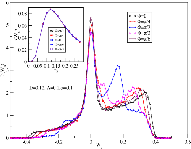
Figure 5: The distribution P(Ws)𝑃subscript𝑊𝑠P(W_{s}) over a single period for various values of initial phase ϕitalic-ϕ\phi. The other parameters are A=0.1𝐴0.1A=0.1, D=0.12𝐷0.12D=0.12 and ω=0.1𝜔0.1\omega=0.1. Inset shows plot of Wsdelimited-⟨⟩subscript𝑊𝑠\langle W_{s}\rangle vs D𝐷D for different value of ϕitalic-ϕ\phi for the same physical parameters.

III Driven nonlinear systems

To this end we consider the motion of a Brownian particle in a bistable system under the action of an external ac force.   The total potential is given by U(x,t)=U0(x)+Up(x,t)𝑈𝑥𝑡subscript𝑈0𝑥subscript𝑈𝑝𝑥𝑡U(x,t)=U_{0}(x)+U_{p}(x,t).  The static double well potential is U0(x)=12x2+14x4subscript𝑈0𝑥12superscript𝑥214superscript𝑥4U_{0}(x)=-\frac{1}{2}x^{2}+\frac{1}{4}x^{4} and the time dependent potential is Up(x,t)=Ax(t)cos(ωt+ϕ)subscript𝑈𝑝𝑥𝑡𝐴𝑥𝑡𝜔𝑡italic-ϕU_{p}(x,t)=-Ax(t)\cos(\omega t+\phi).  This system is shown to exhibit the well known phenomenon of stochastic resonance (SR) [22-28]. Theoretical study on thermodynamic work and heat have been shown to satisfy SSFT [26,27]. Experiments in connection with fluctuation theorems have been carried out in systems exhibiting SR [28,29].  We have numerically evaluated the classical work and thermodynamic work distributions over a single period/large number of periods.  For description of numerical method we refer to [26,27].
Refer to caption
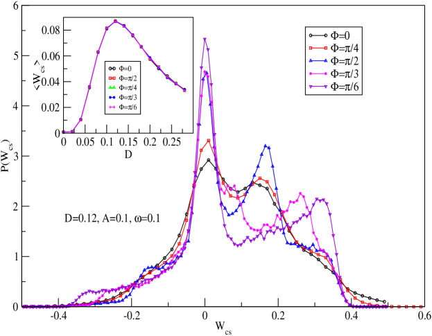
Figure 6: The distribution P(Wcs)𝑃subscript𝑊𝑐𝑠P(W_{cs}) over a single period for various values of initial phase ϕitalic-ϕ\phi. The other parameters are A=0.1𝐴0.1A=0.1, D=0.12𝐷0.12D=0.12 and ω=0.1𝜔0.1\omega=0.1. Inset shows plot of Wcsdelimited-⟨⟩subscript𝑊𝑐𝑠\langle W_{cs}\rangle vs D𝐷D for different values of ϕitalic-ϕ\phi for the same physical parameters.
Refer to caption
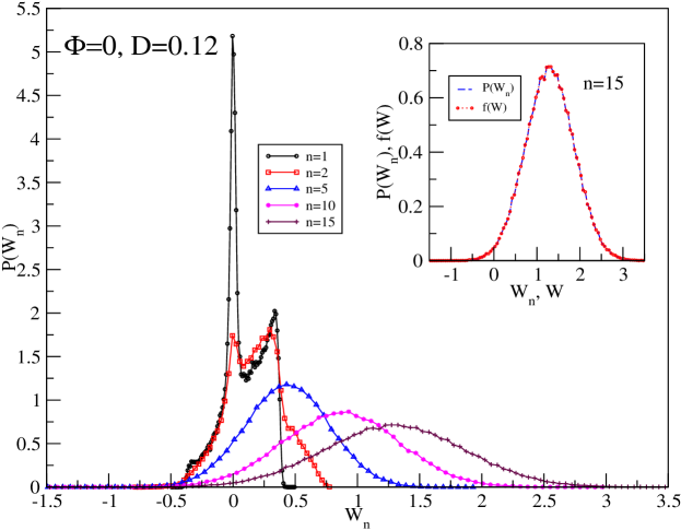
Figure 7: The distributions P(Wn)𝑃subscript𝑊𝑛P(W_{n}) for different periods (n𝑛n) in the time periodic steady state. In the inset P(Wn)𝑃subscript𝑊𝑛P(W_{n}) is plotted along with Gaussian fit f(W)𝑓𝑊f(W) for n=15𝑛15n=15. From the Gaussian fit f(W)𝑓𝑊f(W), the fluctuation ratio has been calculated as σ22βWn=1.022superscript𝜎22𝛽delimited-⟨⟩subscript𝑊𝑛1.022\frac{\sigma^{2}}{\frac{2}{\beta}\langle W_{n}\rangle}=1.022. Here D=0.12𝐷0.12D=0.12, A=0.1𝐴0.1A=0.1 and ω=0.1𝜔0.1\omega=0.1.

In fig(5) and (6) we have plotted probability distributions of thermodynamic work Wssubscript𝑊𝑠W_{s} and classical work Wcssubscript𝑊𝑐𝑠W_{cs} evaluated over a single period in the time periodic regime for various values of initial phases. For a given fixed phase, distributions P(Ws)𝑃subscript𝑊𝑠P(W_{s}) and P(Wcs)𝑃subscript𝑊𝑐𝑠P(W_{cs}) are different. Only for phase ϕ=π2italic-ϕ𝜋2\phi=\frac{\pi}{2}, both distributions are identical. For this particular phase, it can be readily seen that thermodynamic work and classical work are identical when evaluated over a period(s). The multipeaked structure in the distributions arise from the interwell and intrawell dynamics of the particle in a double well system. For details see Ref.[27,28]. Unlike the sensitivity of P(Wcs)𝑃subscript𝑊𝑐𝑠P(W_{cs}) and P(Ws)𝑃subscript𝑊𝑠P(W_{s}), Wsdelimited-⟨⟩subscript𝑊𝑠\langle W_{s}\rangle and Wcsdelimited-⟨⟩subscript𝑊𝑐𝑠\langle W_{cs}\rangle over a cycle do not depend on the initial phase and are identical, i.e., Wcs=Wsdelimited-⟨⟩subscript𝑊𝑐𝑠delimited-⟨⟩subscript𝑊𝑠\langle W_{cs}\rangle=\langle W_{s}\rangle. They are plotted in the inset of fig(5) and (6). Wsdelimited-⟨⟩subscript𝑊𝑠\langle W_{s}\rangle(=Wcsabsentdelimited-⟨⟩subscript𝑊𝑐𝑠=\langle W_{cs}\rangle) exhibits a peak as a function of noise strength D𝐷D. This phenomenon is referred to as SR [25,26,27]. At the value of noise strength corresponding to the peak value in Wcdelimited-⟨⟩subscript𝑊𝑐\langle W_{c}\rangle, the random hops of the Brownian particle between the two wells get synchronized with the external drive[22,28].
Refer to caption
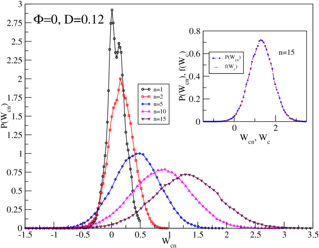
Figure 8: The distributions P(Wcn)𝑃subscript𝑊𝑐𝑛P(W_{cn}) for n𝑛n periods versus Wcnsubscript𝑊𝑐𝑛W_{cn} in the time periodic steady state. Inset shows the plot of P(Wcn)𝑃subscript𝑊𝑐𝑛P(W_{cn}) along with it’s Gaussian fit f(Wc)𝑓subscript𝑊𝑐f(W_{c}) for n=15𝑛15n=15. From the Gaussian fit f(Wc)𝑓subscript𝑊𝑐f(W_{c}), the fluctuation ratio has been calculated as σ22βWcn=1.005superscript𝜎22𝛽delimited-⟨⟩subscript𝑊𝑐𝑛1.005\frac{\sigma^{2}}{\frac{2}{\beta}\langle W_{cn}\rangle}=1.005. The other parameters are same as in fig(7).

In fig(7) and (8), we have plotted P(Wn)𝑃subscript𝑊𝑛P(W_{n}) and P(Wcn)𝑃subscript𝑊𝑐𝑛P(W_{cn}) versus thermodynamic work done over n𝑛n cycles, Wnsubscript𝑊𝑛W_{n} and classical work done over n𝑛n cycles, Wcnsubscript𝑊𝑐𝑛W_{cn} respectively. In both these cases, with increasing n𝑛n, multipeaked distributions become smoother and for large n𝑛n, they both evolve towards Gaussian distribution. Corresponding Gaussian fit for P(Wn)𝑃subscript𝑊𝑛P(W_{n}) and P(Wcn)𝑃subscript𝑊𝑐𝑛P(W_{cn}) for n=15𝑛15n=15 are shown in the inset of fig(7) and (8) respectively. For P(Wn)𝑃subscript𝑊𝑛P(W_{n}) and for n=15𝑛15n=15, from the Gaussian fit we get variance σ2=0.3206superscript𝜎20.3206\sigma^{2}=0.3206, Wn=1.30701delimited-⟨⟩subscript𝑊𝑛1.30701\langle W_{n}\rangle=1.30701 and the corresponding fluctuation ratio, σ22βWn=1.022superscript𝜎22𝛽delimited-⟨⟩subscript𝑊𝑛1.022\frac{\sigma^{2}}{\frac{2}{\beta}\langle W_{n}\rangle}=1.022, which is close to unity (within our numerical accuracy). The Gaussian nature of Wcnsubscript𝑊𝑐𝑛W_{cn} along with fluctuation ratio being 111 implies validity of SSFT. Similar conclusions can be made for P(Wcn)𝑃subscript𝑊𝑐𝑛P(W_{cn}) for n=15𝑛15n=15, where the Gaussian fit gives σ2=0.31525superscript𝜎20.31525\sigma^{2}=0.31525, and hence the fluctuation ratio (1.005) is close to unity. The presence of non-Gaussian tails at large value of Wcnsubscript𝑊𝑐𝑛W_{cn} and Wnsubscript𝑊𝑛W_{n} are not ruled out. However, numerically it is difficult to detect them. It may also be noted that time interval after which SSFT is obeyed for W𝑊W and Wcsubscript𝑊𝑐W_{c} may be different and depends of the physical parameters.

IV Conclusion

We have studied fluctuations in W𝑊W and Wcsubscript𝑊𝑐W_{c} analytically for both transient and time periodic steady states in case of a linear model. We have also shown that as the observation time of trajectories increases, the number of trajectories which exhibit atypical behaviour (namely Wcsubscript𝑊𝑐W_{c} and Q𝑄Q being negative, W𝑊W being less than ΔFΔ𝐹\Delta F) decreases. Thus in the limit of large time of observations, macroscopic thermodynamic behaviour results for physical quantities. We have discussed the validity of SSFT for both W𝑊W and Wcsubscript𝑊𝑐W_{c} in our linear as well as nonlinear models.

V Acknowledgment

One of us (AMJ) thanks DST,  India for financial support. MS thanks Mr. Sourabh Lahiri for his help in computation and Mr. Devashish Sanyal for useful discussions.

VI Appendix-A

Wdelimited-⟨⟩𝑊\displaystyle\langle W\rangle =\displaystyle= A2k4(k2+ω2)[cos(2(ωt+ϕ))cos(2ϕ)]superscript𝐴2𝑘4superscript𝑘2superscript𝜔2delimited-[]2𝜔𝑡italic-ϕ2italic-ϕ\displaystyle\frac{A^{2}k}{4(k^{2}+\omega^{2})}[\cos(2(\omega t+\phi))-\cos(2\phi)] (19)
+\displaystyle+ A2ω2t2(k2+ω2)+A2ω4(k2+ω2)[sin(2(ωt+ϕ)sin(2ϕ)]\displaystyle\frac{A^{2}\omega^{2}t}{2(k^{2}+\omega^{2})}+\frac{A^{2}\omega}{4(k^{2}+\omega^{2})}[\sin(2(\omega t+\phi)-\sin(2\phi)]
+\displaystyle+ A2ω(k2+ω2)2exp(kt)[kcos(ωt+ϕ)+ωsin(ωt+ϕ)](ksin(ϕ)ωcos(ϕ))superscript𝐴2𝜔superscriptsuperscript𝑘2superscript𝜔22𝑘𝑡delimited-[]𝑘𝜔𝑡italic-ϕ𝜔𝜔𝑡italic-ϕ𝑘italic-ϕ𝜔italic-ϕ\displaystyle\frac{A^{2}\omega}{(k^{2}+\omega^{2})^{2}}\exp(-kt)[-k\cos(\omega t+\phi)+\omega\sin(\omega t+\phi)](k\sin(\phi)-\omega\cos(\phi))
+\displaystyle+ A2ω(k2+ω2)2(ksin(ϕ)ωcos(ϕ))(kcos(ϕ)ωsin(ϕ))superscript𝐴2𝜔superscriptsuperscript𝑘2superscript𝜔22𝑘italic-ϕ𝜔italic-ϕ𝑘italic-ϕ𝜔italic-ϕ\displaystyle\frac{A^{2}\omega}{(k^{2}+\omega^{2})^{2}}(k\sin(\phi)-\omega\cos(\phi))(k\cos(\phi)-\omega\sin(\phi))
\displaystyle- A2ωsin(ϕ)k2+ω2[exp(kt){kcos(ωt+ϕ)\displaystyle\frac{A^{2}\omega\sin(\phi)}{k^{2}+\omega^{2}}[\exp(-kt)\{-k\cos(\omega t+\phi)
+\displaystyle+ ωsin(ωt+ϕ)}+(kcos(ϕ)ωsin(ϕ))]\displaystyle\omega\sin(\omega t+\phi)\}+(k\cos(\phi)-\omega\sin(\phi))]

VII Appendix-B

Wcdelimited-⟨⟩subscript𝑊𝑐\displaystyle\langle W_{c}\rangle =\displaystyle= A2k4(k2+ω2)[cos(2(ωt+ϕ))cos(2ϕ)]superscript𝐴2𝑘4superscript𝑘2superscript𝜔2delimited-[]2𝜔𝑡italic-ϕ2italic-ϕ\displaystyle\frac{A^{2}k}{4(k^{2}+\omega^{2})}[\cos(2(\omega t+\phi))-\cos(2\phi)] (20)
+\displaystyle+ A2ω2t2(k2+ω2)+A2ω4(k2+ω2)[sin(2(ωt+ϕ)sin(2ϕ)]\displaystyle\frac{A^{2}\omega^{2}t}{2(k^{2}+\omega^{2})}+\frac{A^{2}\omega}{4(k^{2}+\omega^{2})}[\sin(2(\omega t+\phi)-\sin(2\phi)]
+\displaystyle+ A2ω(k2+ω2)2exp(kt)[kcos(ωt+ϕ)+ωsin(ωt+ϕ)](ksin(ϕ)ωcos(ϕ))superscript𝐴2𝜔superscriptsuperscript𝑘2superscript𝜔22𝑘𝑡delimited-[]𝑘𝜔𝑡italic-ϕ𝜔𝜔𝑡italic-ϕ𝑘italic-ϕ𝜔italic-ϕ\displaystyle\frac{A^{2}\omega}{(k^{2}+\omega^{2})^{2}}\exp(-kt)[-k\cos(\omega t+\phi)+\omega\sin(\omega t+\phi)](k\sin(\phi)-\omega\cos(\phi))
+\displaystyle+ A2ω(k2+ω2)2(ksin(ϕ)ωcos(ϕ))(kcos(ϕ)ωsin(ϕ))superscript𝐴2𝜔superscriptsuperscript𝑘2superscript𝜔22𝑘italic-ϕ𝜔italic-ϕ𝑘italic-ϕ𝜔italic-ϕ\displaystyle\frac{A^{2}\omega}{(k^{2}+\omega^{2})^{2}}(k\sin(\phi)-\omega\cos(\phi))(k\cos(\phi)-\omega\sin(\phi))
+\displaystyle+ A2kk2+ω2sin2(ωt+ϕ)A2ω2(k2+ω2)sin(2(ωt+ϕ))superscript𝐴2𝑘superscript𝑘2superscript𝜔2superscript2𝜔𝑡italic-ϕsuperscript𝐴2𝜔2superscript𝑘2superscript𝜔22𝜔𝑡italic-ϕ\displaystyle\frac{A^{2}k}{k^{2}+\omega^{2}}\sin^{2}(\omega t+\phi)-\frac{A^{2}\omega}{2(k^{2}+\omega^{2})}\sin(2(\omega t+\phi))
+\displaystyle+ A2k2+ω2exp(kt)sin(ωt+ϕ)[ωcos(ϕ)ksin(ϕ)].superscript𝐴2superscript𝑘2superscript𝜔2𝑘𝑡𝜔𝑡italic-ϕdelimited-[]𝜔italic-ϕ𝑘italic-ϕ\displaystyle\frac{A^{2}}{k^{2}+\omega^{2}}\exp(-kt)\sin(\omega t+\phi)[\omega\cos(\phi)-k\sin(\phi)].

VIII Appendix-C

The expression for Δ(τ)Δ𝜏\Delta(\tau) is given by

Δ(τ)=2βWτ2A2ω2kβ(k2+ω2)2(k2cos2(ϕ)ω2sin2(ϕ))(1exp(kτ))Δ𝜏2𝛽delimited-⟨⟩subscript𝑊𝜏2superscript𝐴2superscript𝜔2𝑘𝛽superscriptsuperscript𝑘2superscript𝜔22superscript𝑘2superscript2italic-ϕsuperscript𝜔2superscript2italic-ϕ1𝑘𝜏\displaystyle\Delta(\tau)=\frac{2}{\beta}\langle W_{\tau}\rangle-\frac{2A^{2}{\omega^{2}}}{k\beta(k^{2}+\omega^{2})^{2}}(k^{2}\cos^{2}(\phi)-\omega^{2}\sin^{2}(\phi))(1-\exp(-k\tau)) (21)

IX Appendix-D

The analytical expression for Δ1(τ)subscriptΔ1𝜏\Delta_{1}(\tau) is given by

Δ1(τ)subscriptΔ1𝜏\displaystyle\Delta_{1}(\tau) =\displaystyle= 2βWcτ+2A2ω2kβ(k2+ω2)2(k2cos2(ϕ)ω2sin2(ϕ))(1+exp(kτ))2𝛽delimited-⟨⟩subscript𝑊𝑐𝜏2superscript𝐴2superscript𝜔2𝑘𝛽superscriptsuperscript𝑘2superscript𝜔22superscript𝑘2superscript2italic-ϕsuperscript𝜔2superscript2italic-ϕ1𝑘𝜏\displaystyle\frac{2}{\beta}\langle W_{c\tau}\rangle+\frac{2A^{2}\omega^{2}}{k\beta(k^{2}+\omega^{2})^{2}}(k^{2}\cos^{2}(\phi)-\omega^{2}\sin^{2}(\phi))(1+\exp(-k\tau)) (22)
\displaystyle- 4A2ω2kβ(K2+ω2)2+2A2kβsin2(ϕ)+2A2kβ(k2ω2)(k2+ω2)sin2(ϕ)exp(kτ)4superscript𝐴2superscript𝜔2𝑘𝛽superscriptsuperscript𝐾2superscript𝜔222superscript𝐴2𝑘𝛽superscript2italic-ϕ2superscript𝐴2𝑘𝛽superscript𝑘2superscript𝜔2superscript𝑘2superscript𝜔2superscript2italic-ϕ𝑘𝜏\displaystyle\frac{4A^{2}\omega^{2}k}{\beta(K^{2}+\omega^{2})^{2}}+\frac{2A^{2}}{k\beta}\sin^{2}(\phi)+\frac{2A^{2}}{k\beta}\frac{(k^{2}-\omega^{2})}{(k^{2}+\omega^{2})}\sin^{2}(\phi)\exp(-k\tau)

References

  • (1) C. Bustamante, J. Liphardt and F. Ritort, Physics Today 58, 45 (2005).
  • (2) D.J.Evans and D.J.Searls, Adv.Phys. 51, 1529 (2002).
  • (3) R. J. Harris and G. M. Schütz, J. Stat. Mech. , p07020 (2007).
  • (4) F. Ritort, Sem. Poincare 2, 63 (2003).
  • (5) F. Ritort, J. Phys. Condens. Matter 18, R531 (2006).
  • (6) J. Kurchan, J. Stat. Mech. , p07005 (2007). 
  • (7) D. J. Evans, E. G. D. Cohen and G. P. Morris, Phys. Rev. Lett. 71, 2401 (1993); 71, 3616 (1993) [errata].
  • (8) D. J. Evans and D. J. Searls, Phys. Rev. E 501645 (1994).
  • (9) G. Galvotti and E. G. D. Cohen, Phys. Rev. Lett. 74, 2694 (1995); J. Stat. Phys. 80, 31 (1995).
  • (10) C. Jarzynski, Phys. Rev. Lett. 78 2690(1997).
  • (11) C. Jarzynski, Phys. Rev. E 56 5018 (1997).
  • (12) O. Narayan and A. Dhar, J. Phys. A: Math Gen 37 63(2004).
  • (13) G. E. Crooks, Phys. Rev. E 60, 2721 (1999).
  • (14) G.N. Bochkov and Yu.E.Kuzovlev,  Zh.Eksp.Theor.Fiz. 72, 238 (1977).
  • (15) G.N. Bochkov and Yu.E.Kuzovlev,   Zh.Eksp.Theor.Fiz. 76, 1071 (1979).
  • (16) G.N. Bochkov and Yu.E.Kuzovlev, Physica A,106 443(1981).
  • (17) G.N. Bochkov and Yu.E.Kuzovlev, Physica A,106 480(1981).
  • (18) Udo Seifert, Phys. Rev. Lett. 95,040602 (2005).
  • (19) Udo Seifert, Eur. Phys. J. B 64, 423 (2008).
  • (20) C.Jarzynski, C.R. Physique 8, 495 (2007).
  • (21) C. Jarzynski, Eur. Phys. J. B 64, 331 (2008).
  • (22) L. Gammaitoni, P. Hanggi, P. Jung and F. Marchesoni, Rev.Mod. Phys.70 223(1998).
  • (23) T. Wellens, V. Shatokhin and A. Buchleitner, Rep. Prog. Phys. 67 45(2005).
  • (24) M.C. Mahato and A.M. Jayannavar, Physica A 248 138(1998).
  • (25) D. Dan and A.M. Jayannavar, Physica A 345 404 (2005).
  • (26) S. Saikia, R. Roy and A.M. Jayannavar, Physics Letters A 369 367 (2007).
  • (27) M.Sahoo, S.Saikia and A.M. Jayannavar, Physica A 387 6284(2008).
  • (28) P. Jop, A. Petrosyan and S. Ciliberto, Europhysics Lett. 81 50005(2008).
  • (29) A. Imparto, P. Jop, A. Petrosyan and S. Ciliberto, J. Stat. Mech. P10017 (2008).
  • (30) H. Risken, The Fokker-Planck Equation, Springer-Verlag, Berlin, (1984).
  • (31) R. van Zon and E.G.D. Cohen, Phys. Rev. E 67 046102(2002).
  • (32) A.M. Jayannavar and M. Sahoo, Phys. Rev. E 75 032102 (2007).
  • (33) A. M. Jayannavar and M. Sahoo, Pramana J.Phys. 70 201 (2008).
  • (34) K. Sekimoto, J. Phys. Soc. Jpn. 66 6335(1997).
  • (35) A.Saha, S.Lahiri and A.M. Jayannavar unpublished.