$(n+1)$-Dimensional Lorentzian Wormholes in an Expanding Cosmological Background

Abstract

We discuss $(n+1)$-dimensional dynamical wormholes in an evolving cosmological background with a throat expanding with time. These solutions are examined in the general relativity framework. A linear relation between diagonal elements of an anisotropic energy-momentum tensor is used to obtain the solutions. The energy-momentum tensor elements approach the vacuum case when we are far from the central object for one class of solutions. Finally, we discuss the energy-momentum tensor which supports this geometry, taking into account the energy conditions .

I Introduction

Wormholes are hypothetical objects which connect two distant parts of the same spacetime or two different spacetimes by a throat-like object which has the minimum radius of the spacetime. Although a wormhole solution first entered the physics literature in 1916 reff , the concept was first considered seriously in 1935 by Einstein and Rosen 1 which was later called Einstein-Rosen bridge but the word wormhole was first time coined by wheeler 2 in 1957. A more interesting analysis of wormholes was performed by Morris and Thorne in 1988 and they presented a new kind of wormhole (traversable wormhole) for the first time 3 . It was known from before that matter we need to support such a geometry violates the weak and strong energy conditions near the throat 4 ; 5 . Morris and Thorne reconsidered these conditions for a traversable wormhole 3 . Since the matter that supports this geometry doesn’t satisfy the common energy conditions they called it ’exotic’. An example of exotic matter is matter with negative energy density 3 .

Another property of these wormholes is the possibility of transforming them into time machines for backward time traveling 6 ; 7 and thereby, perhaps for causality violation by closed timelike curves. Teo 8 found that the null energy condition ($NEC$) is violated by stationary, axially symmetric, traversable wormholes but there can be classes of geodesics which do not cross energy condition violating regions. Another case of evolving wormholes may alter this situation9 ; 10 . It is known that we can have violations of weak energy condition ($WEC$) due to some quantum mechanical effects (such as Casimir effect) 11 . If we search for this effect in the history of evolving cosmos, we can find such a situation at the quantum cosmological era when quantum gravity is dominant. Following the inflation theory by A. Guth 12 it has been supposed that non-trivial topological objects such as microscopic wormholes may have been formed during that era and then enlarged to macroscopic objects with expansion of the universe 13 ; 14 ; 10 ; 15 . Although most studies have focused on four dimensions, with the advent of string theory that demands higher dimensional spacetimes, it is natural to examine the possibility of wormholes beyond the ordinary four dimensions. Euclidean wormholes in string theory have recently been studied 16 ; 17 ; 18 ; 19 ; 20 as solutions of supergravities. With this motivation, we are going to choose the generalized Friedmann-Robertson-Walker ($FRW$) metric in $(n+1)$-dimensions and investigate exact Lorentzian wormhole geometries with spherically symmetry.

This paper is organized in the following manner: In sec. II we present the ansatz metric and the resulting solutions in 4-dimensions. In section III, we extend the solutions to (n+1)-dimensions. In section IV, we investigate the corresponding energy-momentum tensor and determine the exoticity parameter. The last section is devoted to conclusions and closing remarks.

II Field Equations

It is very common today that we start studying cosmology with the so-called ’cosmological principle’. It states that the universe at large scale is homogeneous and isotropic. With this assumption, we find out that the metric we need to demonstrate such a spacetime in 4-dimensions is as follows

$$ds^{2}=-dt^{2}+R(t)^{2}\left[\frac{dr^{2}}{1-kr^{2}}+r^{2}(d\theta^{2}+sin^{2}\theta\,d\phi^{2})\right],$$ (1)

which is known as the Robertson-Walker (RW) metric 21 . The coordinate system $(r,\theta,\phi)$ used here is the so-called ’co-moving coordinate system’. $R(t)$ is the scale factor and the only dynamical parameter to determine. $k=0,\pm 1$ correspond to spatially flat, closed and open spacetimes respectively. This metric contains a high degree of symmetry which is demonstrated by its six killing vectors.

For our aim, we need to generalize this metric to $(n+1)$-dimensions and reduce its symmetry. We break its homogeneity by replacing $1/(1-kr^{2})$ with $1+a(r)$. This metric is still isotropic about $r=0$ but not necessarily homogeneous. We therefore write our ansatz metric as

$$ds^{2}=-dt^{2}+R(t)^{2}\left[(1+a(r))\,dr^{2}+r^{2}d\Omega_{n-1}^{2}\right],$$ (2)

where $a(r)$ is an unknown function. It is clear that the Robertson-Walker metric is a special case of this metric. With this ansatz metric, we look at our equations. We start with $n=4$ and then extend the solutions to arbitrary $n$. In the first step we write our ansatz metric for 5-dimensions (n=4)

$$ds^{2}=-dt^{2}+R(t)^{2}\left[(1+a(r))\,dr^{2}+r^{2}(d\theta^{2}+sin^{2}\theta\,(d\phi^{2}+sin^{2}\phi\,d\psi^{2})\right].$$ (3)

The non-vanishing components of the Einstein tensor for our ansatz metric read

$$\mathit{G_{t}^{t}}=-{\displaystyle\frac{6\,\mathrm{\dot{R}}^{2}}{\mathrm{R}^{2}}}-\frac{3}{2}{\displaystyle\frac{r\,\mathrm{a^{\prime}}+\mathrm{2a}(1+\mathrm{a})}{\mathrm{R}^{2}\,r^{2}\,(1+\mathrm{a})^{2}}},$$ (4)

$$\mathit{G_{r}^{r}}=-3(\frac{R\ddot{R}+\dot{R}^{2}}{R^{2}})-3\frac{a}{R^{2}r^{2}(1+a)},$$ (5)

$$\mathit{G_{\theta}^{\theta}}=-3(\frac{R\ddot{R}+\dot{R}^{2}}{R^{2}})-\frac{ra^{\prime}+a(1+a)}{R^{2}r^{2}(1+a)^{2}},$$ (6)

$$G_{\theta}^{\theta}=G_{\phi}^{\phi}=...,$$ (7)

in which ’dot’ is derivative with respect to $t$, while ’prime’ is derivative with respect to $r$.

Such a geometry is supported by an anisotropic, diagonal energy-momentum tensor:

$$\rho=-\frac{1}{8\pi G}T_{t}^{t}=\frac{1}{8\,{\pi\,G}}\,\left[{\displaystyle\frac{6\,\mathrm{\dot{R}}^{2}}{\mathrm{R}^{2}}}+\frac{3}{2}{\displaystyle\frac{r\,\mathrm{a^{\prime}}+\mathrm{2a}(1+\mathrm{a})}{\mathrm{R}^{2}\,r^{2}\,(1+\mathrm{a})^{2}}}\right],$$ (8)

$$P_{r}=\frac{1}{8\pi G}T_{r}^{r}=\frac{1}{8\pi G}\left[-3(\frac{R\ddot{R}+\dot{R}^{2}}{R^{2}})-3\frac{a}{R^{2}r^{2}(1+a)}\right],$$ (9)

$$P_{t}=\frac{1}{8\pi G}T_{\theta}^{\theta}=\frac{1}{8\pi G}\left[-3(\frac{R\ddot{R}+\dot{R}^{2}}{R^{2}})-\frac{ra^{\prime}+a(1+a)}{R^{2}r^{2}(1+a)^{2}}\right].$$ (10)

In these relations $P_{t}$ and $P_{r}$ are the transverse and radial pressures, respectively.

Here, we assume the following equation of state

$$\rho=-{\displaystyle\frac{\mathit{P_{r}}+\gamma\,\mathit{P_{t}}}{1+\gamma}},$$ (11)

where $\gamma$ depends on $n$ the dimension of the space. This equation reduces to the vacuum equation of state $P=-\rho$ when $P_{r}=P_{t}$.

Using equations (8-10) and relation (11) in 5-dimensions (n=4), we obtain:

$$\left[{\displaystyle\frac{6\,\mathrm{\dot{R}}^{2}}{\mathrm{R}^{2}}}+\frac{3}{2}{\displaystyle\frac{r\,\mathrm{a^{\prime}}+\mathrm{2a}(1+\mathrm{a})}{\mathrm{R}^{2}\,r^{2}\,(1+\mathrm{a})^{2}}}\right]+$$ (12)

$$\frac{1}{1+\gamma}\left[\left[-3(\frac{R\ddot{R}+\dot{R}^{2}}{R^{2}})-3\frac{a}{R^{2}r^{2}(1+a)}\right]+\gamma\left[-3(\frac{R\ddot{R}+\dot{R}^{2}}{R^{2}})-\frac{ra^{\prime}+a(1+a)}{R^{2}r^{2}(1+a)^{2}}\right]\right]=0.$$

Fortunately, this equation can be separated into radial and temporal equations.

$$6R\ddot{R}-6\dot{R}^{2}=\frac{(\gamma+3)ra^{\prime}+4\gamma a(1+a)}{r^{2}(1+\gamma)(1+a)^{2}}$$ (13)

This equation can be easily solved and has the following solutions:

$$R(t)=\frac{1}{2}\sqrt{\frac{-1}{C_{4}}}(e^{(\frac{t}{C_{2}})}+e^{(-\frac{t}{C_{2}})}),$$ (14)

$$1+a(r)=\frac{1}{1+\frac{C_{4}}{C^{2}_{2}}r^{2}+C_{1}r^{-(\frac{4\gamma}{3+\gamma})}}.$$ (15)

The energy-momentum tensor needed to support this geometry has the following components:

$$\rho=\frac{3}{4\pi GC_{2}^{2}}-\frac{3r^{-\frac{6(\gamma+1)}{\gamma+3}}C_{1}(\gamma-3)}{2\pi GC_{4}(e^{(\frac{t}{C_{2}})}+e^{(-\frac{t}{C_{2}})})^{2}(\gamma+3)},$$ (16)

$$P_{r}=-\frac{3}{4\pi GC_{2}^{2}}-\frac{3r^{-\frac{6(\gamma+1)}{\gamma+3}}C_{1}}{2\pi GC_{4}(e^{(\frac{t}{C_{2}})}+e^{(-\frac{t}{C_{2}})})^{2}},$$ (17)

and

$$P_{t}=-\frac{3}{4\pi GC_{2}^{2}}+\frac{3r^{-\frac{6(\gamma+1)}{\gamma+3}}C_{1}(\gamma-1)}{2\pi GC_{4}(e^{(\frac{t}{C_{2}})}+e^{(-\frac{t}{C_{2}})})^{2}(\gamma+3)}.$$ (18)

III $(n+1)$-Dimensional solutions

The solutions we obtained in 5-dimensional spacetime can be easily extended to $(n+1)$-dimensions. The resulting solutions in (n+1)-dimensions read

$$R(t)=\frac{1}{2}\sqrt{\frac{-1}{C_{4}}}(e^{(\frac{t}{C_{2}})}+e^{(-\frac{t}{C_{2}})}),$$ (19)

$$1+a(r)=\frac{1}{1+\frac{C_{4}}{C^{2}_{2}}r^{2}+C_{1}r^{(\frac{2\gamma(-n+2)}{n+\gamma-1})}}.$$ (20)

Following these solutions, the energy-momentum tensor which supports this structure in (n+1)-dimensions will be:

$$\rho=\frac{A}{\pi GC_{2}^{2}}-\frac{Br^{-\frac{(2n-2)(\gamma+1)}{\gamma+n-1}}C_{1}(\gamma-n+1)}{\pi GC_{4}(e^{(\frac{t}{C_{2}})}+e^{(-\frac{t}{C_{2}})})^{2}(\gamma+n-1)},$$ (21)

$$P_{r}=-\frac{A}{\pi GC_{2}^{2}}-\frac{Br^{-\frac{(2n-2)(\gamma+1)}{\gamma+n-1}}C_{1}}{\pi GC_{4}(e^{(\frac{t}{C_{2}})}+e^{(-\frac{t}{C_{2}})})^{2}},$$ (22)

$$P_{t}=-\frac{A}{\pi GC_{2}^{2}}+\frac{Br^{-\frac{(2n-2)(\gamma+1)}{\gamma+n-1}}C_{1}(\gamma-n+3)}{\pi GC_{4}(e^{(\frac{t}{C_{2}})}+e^{(-\frac{t}{C_{2}})})^{2}(\gamma+n-1)}.$$ (23)

As a check for the correctness of these solutions one can see that they reduce to the solutions of 15 for n=3 with proper definition for the integration constants.

III.1 Properties of the Solutions

Now let us have a look at radial behavior of the solutions. In the paper by Morris and Thorne 3 , the metric of the wormhole is written in the form:

$$\mathit{\ ds}^{2}=-\mathit{\ d}\,t^{\mathit{2\ }}+{\displaystyle\frac{\mathit{\ d}\,r^{\mathit{2\ }}}{1-{\displaystyle\frac{\mathrm{b}(r)}{r}}}}+r^{2}\,(\mathit{\ d}\,\theta^{\mathit{2\ }}+\mathrm{sin}(\theta)^{2}\,\mathit{\ d}\,\phi^{\mathit{2\ }}).$$ (24)

In which $b(r)$ is the shape function and the throat radius satisfies $b(r_{0})=r_{0}$. If the equation $d(r)=r-b(r)$ has any root $r_{0}$ and simultaneously $d(r)>0$ for $r>r_{0}$ then we will have a wormhole and $r_{0}$ gives the throat radius of the wormhole. In our solutions, with choosing $\gamma=n-1$ the condition for the existence of wormholes will be

$$\mathrm{d}(r)=r+\alpha r^{3}+\beta r^{3-n}=0\ \ {\rm at}\ \ r=r_{0},$$ (25)

and

$$\mathrm{d}(r)=r+\alpha r^{3}+\beta r^{3-n}>0\ \ {\rm for}\ \ r>r_{0},$$ (26)

where $\alpha$ and $\beta$ are constants related to the integration constants:

$$\alpha=\frac{C_{4}}{C_{2}^{2}},\ \ \beta=C_{1}.$$ (27)

Solving equation (25) analytically is not possible except for special values of n, as presented in 15 for n=3. Then for investigating the properties of the solutions, we plot $d(r)$ against $r$ in Figure (1-2). We classify the solutions in the following manner:

Figure 1: The behavior of $1+a(r)$ and $d(r)$ for $\gamma=3$ and (a) $\alpha=1,\beta=-1,n=4$, (b) $\alpha=-0.23,\beta=-1,n=4$, (c) $\alpha=-1,\beta=1,n=4$

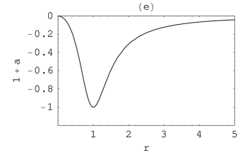
Figure 2: The behavior of $1+a(r)$ and $d(r)$ for $\gamma=3$ and (d) $\alpha=-1,\beta=0,n=4$, (e) $\alpha=-1,\beta=-1,n=4$, (f) $\alpha=1,\beta=1,n=4$, (g) $\gamma=-5,\alpha=1,\beta=-1,n=4$

In the case (a), $\alpha=1$ and $\beta=-1$, we see from Fig.1 that we have a lower limit on $r$ which corresponds to the throat radius of the wormhole and we see also that there is no upper limit on $r$ which reminds us that we have an open spacetime.

For the choice (b), $\alpha=-0.23$ and $\beta=-1$, we have lower and upper limits on $r$. The lower limit corresponds to the throat radius of the wormhole and the upper limit signifies a closed spacetime.

In the cases (a) and (b), the Kretschman scalar blows up at $r=0$ but, this point is not included in our physical spacetime with proper signature.

Case (c), $\alpha=-1$ and $\beta=1$ represents a naked singularity in a closed cosmological background, because the Kretschman scalar blows up at the origin ($r=0$).

Case (d), $\beta=0$ and $\alpha=\pm 1$ leads to $1+a(r)=1/(1\pm r^{2})$, which corresponds to the $k=\mp 1$ $FRW$ metric.

Case (e), $\alpha=-1$ and $\beta=-1$, $1+a(r)$ becomes negative and the metric’s signature is not of cosmological interest.

And finally, (f), $\alpha=1$ and $\beta=1$, $1+a(r)$ is regular everywhere and represent a naked singularity, again but in an open universe.

We can also have a discussion on the cases which include $\gamma<0$. For case $\gamma=-5$, from (20) we obtain

$$d(r)=r+\alpha r^{3}+\beta r^{\frac{11n-26}{n-6}}.$$ (28)

This equation with $\alpha=1$ and $\beta=-1$, leads to a wormhole centered, open universe which is illustrated in Fig.2 part (g).

It is worth having a look at the Ricci scalar ($\cal R$). In (n+1)-dimensional spacetime $\cal R$ is:

$${\cal R}=\frac{n(n+1)}{C_{2}^{2}}-\frac{Wr^{(\frac{-(2n-2)(1+\gamma)}{\gamma+n-1})}C_{1}(\gamma-n+1)}{(e^{(\frac{t}{C_{2}})}+e^{(-\frac{t}{C_{2}})})^{2}C_{4}(\gamma+n-1)}.$$ (29)

We can see that choosing $C_{1}=0$ or $\gamma=n-1$, constant curvature spacetime is retrieved. In the case $C_{1}=0$, we have a maximally symmetric de Sitter spacetime. We expect this result because, we see that the constant part of the Ricci scalar reminds us a maximally symmetric spacetime curvature.

The wormholes discussed in this paper are traversable. We present two reasons here. The first reasoning is based on the redshift of a signal emitted at the comoving coordinate $r_{1}$ and received by a distant observer. Using the metric (3) and for a radial beam, we obtain

$$\frac{dt}{R(t)}=(1+a(r))dr.$$ (30)

Using this relation for two signals separated by $\tau_{0}$ in time when emitted (and $\tau$ when detected), we obtain

$$\frac{\tau}{\tau_{0}}=1+z=\frac{R(t_{0})}{R(t_{1})},$$ (31)

in which $R(t_{0})$ is the scale factor at the time of observation, and $R(t_{1})$ is the scale factor at the time of emission. This leads to the exactly same relation as the cosmological redshift relation which shows that the wormhole does not introduce extra (local) redshift. Light signals, therefore can travel to the both sides of the throat and there is no horizon.

The second is based on the geodesic equation, which -for the metric (3)- leads to

$$\frac{d^{2}r}{d\lambda^{2}}+\frac{1}{2}\frac{a^{\prime}(r)}{1+a(r)}\left(\frac{dr}{d\lambda}\right)^{2}+2\frac{\dot{R}}{R}\frac{dt}{d\lambda}\frac{dr}{d\lambda}=0$$ (32)

and

$$\frac{d^{2}t}{d\lambda^{2}}+R\dot{R}(1+a(r))\left(\frac{dr}{d\lambda}\right)^{2}=0,$$ (33)

in which $\lambda$ is an affine parameter along the geodesic.

The first equation has the following first integral

$$\frac{dr}{d\lambda}=\frac{C}{R^{2}\sqrt{1+a(r)}}.$$ (34)

Since the proper distant element is $\delta l=R\sqrt{1+a}\delta r$, we see that there is no radial turning point and any particle can move in either radial directions at any point near to the wormhole, which clearly shows that the wormhole is traversable.

Let us have a brief discussion on the observational consequences of these solutions. We can have a variety of geodesics in a wormhole spacetime Riazinasr . Geodesics can pass through the throat right to the other part of the spacetime (the parallel universe), or be deflected back to the same universe. As pointed out by Cramer et. al. cramer , it should be possible -in principle- to detect wormholes via the gravitational lensing they cause. This, however, depends on the wormhole being stable, which is not addressed in the present paper.

IV Energy-Momentum Tensor and Exoticity Parameter

The $(n+1)$-dimensional version of diagonal elements of the energy- momentum tensor are were given in equations (21-23).

Some points are interesting to mention about the energy-momentum tensor. Since we are looking for spherical structures in a cosmological background, $P_{t}$, $P_{r}$ and $\rho$ should become almost $r$-independent at large $r$. In particular, for suitable values of $\gamma$, the solutions approach $P_{r}=P_{t}=-\rho=constant$ which correspond to dark energy (cosmological constant). The second point is the conservation equation of the energy-momentum tensor:

$$\ D_{\mu}T^{\mu\nu}=0$$ (35)

which leads to

$$\partial_{t}\rho+n\rho+P_{r}+(n-1)P_{t}=0.$$ (36)

Our solutions satisfy this equation, as expected.

Let us now investigate the exoticity parameter. For an isotropic fluid, the energy-momentum tensor is in the form $T_{\nu}^{\mu}={\rm diag}(-\rho,P,...,P)$ and the exoticity parameter is defined according to

$$\xi=-\frac{\rho+P}{\rho},$$ (37)

where $\xi>0$ corresponds to the exotic matter and $\xi<0$ to the non-exotic matter. Since we have an anisotropic medium, the energy-momentum tensor has the form $T_{\nu}^{\mu}={\rm diag}(-\rho,P_{r},P_{t},...,P_{t})$. We therefore take the average pressure

$$\bar{P}=\frac{1}{n}(P_{r}+(n-1)P_{t}).$$

Taking this into account, we adopt the following, more general definition for $\bar{P}$:

$$\bar{P}=\frac{P_{r}+\gamma P_{t}}{\gamma+1},$$

and modify (37) according to

$$\bar{\xi}=-\frac{\rho+\bar{P}}{\rho}.$$ (38)

From (11) we see that the modified exoticity parameter is everywhere zero and for all cases, which shows that we are on the border line between exotic and non-exotic matter according to the criterion. The weak energy condition $(WEC)$ requires

$$T_{\mu\nu}u^{\mu}u^{\nu}\geq 0$$ (39)

for every nonspacelike $u^{\mu}$ which leads to 22

$$\rho\geq 0,\ \ \rho+P_{r}\geq,\ \rho+P_{t}\geq 0.$$ (40)

These equations and relations (21-23) lead to

$$\rho\geq 0\Rightarrow{\displaystyle\frac{A}{G\,\pi\,\mathit{C_{2}}^{2}}}-{\displaystyle\frac{B\,r^{(-\frac{(2\,n-2)\,(\gamma+1)}{\gamma+n-1})}\,\mathit{C_{1}}\,(\gamma+1-n)}{\mathit{C_{4}}\,\pi\,G\,(\gamma+n-1)\,(e^{(\frac{t}{\mathit{C_{2}}})}+e^{(-\frac{t}{\mathit{C_{2}}})})^{2}}}\geq 0,$$ (41)

$$\rho+P_{r}\geq 0\Rightarrow-\frac{2\,B\,C_{1}\,\gamma\,r^{-\frac{(2n-2)(\gamma+1)}{\gamma+n-1}}}{C_{4}\pi G(\gamma+n-1)(e^{(\frac{t}{C_{2}})}+e^{(-\frac{t}{C_{2}})})^{2}}\geq 0,$$ (42)

$$\rho+P_{t}\geq 0\Rightarrow\frac{2\,B\,C_{1}\,r^{-\frac{(2n-2)(\gamma+1)}{\gamma+n-1}}}{C_{4}\pi G(\gamma+n-1)(e^{(\frac{t}{C_{2}})}+e^{(-\frac{t}{C_{2}})})^{2}}\geq 0.$$ (43)

These relations show that, with the choice $\gamma\geq 0$, we can’t have any wormhole without violating $WEC$, or at least the border line at which we have the equality relation in (42) and (43). In the case $\gamma<0$ the relations (42) and (43) are both simultaneously satisfied and we have to investigate the relation (41) in order to see wether $WEC$ is satisfied. It is interesting to note that for particular ranges of constants we have wormhole solutions which satisfy $WEC$ throughout the spacetime. As an example of these solutions one can see case (g) in Fig.2.

V Summary and conclusion

We introduced time-dependent wormholes in an $(n+1)$-dimensional expanding cosmological background. We presented an ansatz metric and a linear relation between the diagonal elements of the energy-momentum tensor. With these assumptions, we separated and solved the field equations. Solutions were classified into different categories with distinct geometries for the central object. We distinguished two classes of solutions which represented Lorentzian wormholes with expanding throat in closed and open universes. We also found two classes of solutions that contain an intrinsic singularity in open and closed universes. The other interesting solution was the familiar maximally symmetric de Sitter spacetimes. The Ricci scalar was calculated and the constant curvature class of solutions were discussed. The issue of the traversability of the wormhole solutions was considerd. We investigated the energy-momentum tensor required to support these solutions. Our solutions led to an energy-momentum tensor which approaches the cosmological constant case far from the wormhole for $\gamma\geq 0$. Finally, we investigated the exoticity parameter. The exoticity parameter for the linear equation of state is zero everywhere which is border line between exotic and non-exotic matter. We also checked the weak energy condition and found that the weak energy condition in the choice $\gamma\geq 0$ is violated except for the border line case. For the case $\gamma<0$, $WEC$ is satisfied for suitable values of constants.

References

• (1) Ludwig Flamm, Physik. Zeitschr. 17, 448 (1916).
• (2) A. Einstein, N. Rosen, Phys.Rev. 48,73 (1935).
• (3) J. A. Wheeler, Ann. Phys. 2,604 (1957).
• (4) M. S. Morris, K. S. Thorne , Am.J. Phys. 56 (1988) 395.
• (5) A. Borde, Class. Gravitation 4, 343 (1987).
• (6) S. W. Hawking, Phys.Rev. D 46, 603 (1992).
• (7) M. S. Morris, K. S. Thorne and U. Yurtsever, Phys. Rev. Lett. 61, 1446 (1988).
• (8) V. P. Frolov and I. D. Novikov, Phys. Rev. D 42, 1057 (1990).
• (9) E. Teo, Phys.Rev. D 58, 024014 (1998).
• (10) S. Kar, D. Sahdev , gr-qc/9506094v3.
• (11) N. Riazi, B. Nasr, Astrophys. Space Sci. 271,237(2000).
• (12) H. Epstein, V. Glaser, A. Jaffe, Nuvo Cimento 36, 1016 (1965).
• (13) A. H. Guth, Phys.Rev. D 23, 347 (1981).
• (14) T. A. Roman, Phys. Rev. D 47, 1370 (1993).
• (15) N. Riazi, J. Korean Astron. Soc.29, S283 (1996).
• (16) N. Riazi, Astrophys. Space Sci. 283, 231 (2003).
• (17) J.M. Maldacena and L. Maoz, JHEP 0402, 053 (2004).
• (18) E. Bergshoeff, A. Collinucci, A. Ploegh, S. Vandoren and T. Van Riet, JHEP 0601, 061 (2006).
• (19) N. Arkani-Hamed, J. Orgera and J. Polchinski, JHEP 0712, 018 (2007).
• (20) A. Bergman and J. Distler, hep-th/0707.3168.
• (21) E. Bergshoeff, W. Chemissany, A. Ploegh, M. Trigiante and T. Van Riet, hep-th/0806.2310.
• (22) S. Weinberg, Gravitation and Cosmology, John Wiley and Sons, USA (1972).
• (23) N. Riazi, B. Nasr, Iranian Journal of Science and Technology , 24, No.2, Trans.A, 139 (2000).
• (24) John G. Cramer, Robert L. Forward, et. al, Phys. Rev. D 51, 3117 (1995).
• (25) S. Carroll, Spacetime and Geometry : An Introduction to General Relativity, Addison Wesley, USA (2004).