Nuclear fusion reaction rates for strongly coupled ionic mixtures

Abstract

We analyze the effect of plasma screening on nuclear reaction rates in dense matter composed of atomic nuclei of one or two types. We perform semiclassical calculations of the Coulomb barrier penetrability taking into account a radial mean field potential of plasma ions. The mean field potential is extracted from the results of extensive Monte Carlo calculations of radial pair distribution functions of ions in binary ionic mixtures. We calculate the reaction rates in a wide range of plasma parameters and approximate these rates by an analytical expression that is expected to be applicable for multicomponent ions mixtures. Also, we analyze Gamow-peak energies of reacting ions in various nuclear burning regimes. For illustration, we study nuclear burning in ¹²C–¹⁶O mixtures.

I Introduction

Nuclear fusion in dense stellar matter is most important for the evolution of all stars. The main source of energy for main-sequence stars is provided by hydrogen and helium burning. Subsequent burning of carbon and heavier elements clayton83 drives an ordinary star along the giant/red-giant branch to its final moments as a normal star. Nuclear burning is also important for compact stars. It is the explosive burning of carbon and other elements in the cores of massive white dwarfs; it triggers type Ia supernova explosions (see, e.g., hoeflich06 and references therein). Explosive burning in the envelopes of neutron stars can produce type I X-ray bursts sb06 and superbursts (that are observed from some X-ray bursters; e.g., Refs. cummingetal05 ; guptaetal06 ). Accreted matter which penetrates into deeper layers of the neutron star crust undergos pycnonuclear reactions. They can power thermal radiation observed from neutron stars in soft X-ray transients in quiescent states (see, e.g., Refs. YL03 ; Transient03 ; Transient04 ; YLG05 ; guptaetal06 ; pgw06 ; lh07 ; shternin07 ; YakPycno06 ). Thus, nuclear reactions are important in stars at all evolutionary stages.

It is well known that nuclear reaction rates in dense matter are determined by astrophysical $S$-factors, which characterize nuclear interaction of fusing atomic nuclei, and by Coulomb barrier penetration preceding the nuclear interaction. We will mostly focus on the Coulomb barrier penetration problem. Fusion reactions in ordinary stars proceed in the so called classical thermonuclear regime in which ions (atomic nuclei) constitute a nearly ideal Boltzmann gas. In this case the Coulomb barrier between reacting nuclei is almost unaffected by plasma screening effects produced by neighboring plasma particles. The Coulomb barrier penetrability is then well defined.

However, in dense matter of white dwarf cores and neutron star envelopes the ions form a strongly non-ideal Coulomb plasma, where the plasma screening effects can be very strong. The plasma screening greatly influences the barrier penetrability and the reaction rates. Depending on density and temperature of the matter, nuclear burning can proceed in four other regimes svh69 . They are the thermonuclear regime with strong plasma screening, the intermediate thermo-pycnonuclear regime, the thermally enhanced pycnonuclear regime, and the pycnonuclear zero-temperature regime. The reaction regimes will be briefly discussed in Sec. II.1. In these four regimes the calculation of the Coulomb barrier penetration is complicated. There have been many attempts to solve this problem using several techniques but the exact solution is still a subject of debates (see Gasques_etal05 ; YGABW06 ; OCP_react and reference therein).

In our previous paper OCP_react we studied nuclear reactions in a one component plasma (OCP) of ions. Now we extend our consideration to binary ionic mixtures(BIMs). In Sec. II we discuss physical conditions and reaction regimes. In Sec. III we describe the results of our most extensive and accurate Monte Carlo calculations, analyze them and use to parameterize the mean-field potential. In Sec. IV this potential is employed to calculate the enhancement factors of nuclear reaction rates. We study the Gamow peak energies and the effects of plasma screening on astrophysical $S$-factors in Sec. V. Section VI is devoted to the analysis of the results. We conclude in Sec. VII. In the Appendix we suggest a simple generalization of our results to the cases of weak and moderate Coulomb coupling of ions.

II Physical conditions and reaction regimes

II.1 Nuclear reaction regimes

We consider nuclear reactions in dense matter of white dwarf cores and outer envelopes of neutron stars. This matter contains atomic nuclei (ions, fully ionized by electron pressure) and strongly degenerate electrons, which form an almost uniform background of negative charge. For simplicity, we will not consider the inner crust of neutron stars (with density higher than the neutron drip density $\sim 4\times 10^{11}$ g cm^-3 NV73 ), which contains also free degenerate neutrons.

We will generally study a multicomponent mixture of ions $j=1,2,\ldots$ with atomic mass numbers $A_{j}$ and charge numbers $Z_{j}$. The total ion number density can be calculated as $n_{\mathrm{i}}=\sum_{j}\,n_{j}$, where $n_{j}$ is a number density of ions $j$. It is useful to introduce the fractional number $x_{j}=n_{j}/n_{\mathrm{i}}$ of ions $j$. Let us also define the average charge number $\langle Z\rangle=\sum_{j}\,x_{j}Z_{j}$ and mass number $\langle A\rangle=\sum_{j}\,x_{j}A_{j}$ of ions. The charge neutrality implies that the electron number density is $n_{e}=\langle Z\rangle n_{\mathrm{i}}$. The electron contribution to the mass density $\rho$ can be neglected, so that $\rho\approx\langle A\rangle m_{\mathrm{u}}n$, where $m_{\mathrm{u}}\approx 1.66054\times 10^{-24}$ g is the atomic mass unit.

The importance of the Coulomb interaction for ions $j$ can be described by the coupling parameter $\Gamma_{j}$

$$\Gamma_{j}=\Gamma_{jj}=\frac{Z_{j}^{2}\,e^{2}}{a_{j}k_{\mathrm{B}}T},\quad a_{j}=Z_{j}^{1/3}a_{\mathrm{e}},\quad a_{\mathrm{e}}=\left(\frac{3}{4\pi n_{\mathrm{e}}}\right)^{1/3},$$ (1)

where $a_{j}$ and $a_{\mathrm{e}}$ are the ion-sphere and electron-sphere radii, $k_{\mathrm{B}}$ is the Boltzmann constant, and $T$ is the temperature. Note, that the electron charge within an ion sphere exactly compensates the ion charge $Z_{j}e$; $\Gamma_{j}$ gives the ratio of characteristic electrostatic energy $Z_{j}^{2}e^{2}/a_{j}$ to the thermal energy $k_{\mathrm{B}}T$.

If $\Gamma_{j}\ll 1$, the ions constitute an almost ideal Boltzman gas, while for $\Gamma_{j}\gtrsim 1$ they are strongly coupled by Coulomb forces and constitute either a Coulomb liquid or solid. The transformation from the gas to the liquid at $\Gamma_{j}\sim 1$ is smooth, without any phase transition. According to highly accurate Monte Carlo calculations, a classical OCP of ions solidifies at $\Gamma\approx 175$ (see, e.g. DWSBY2001 ).

We will discuss fusion reactions

$$(A_{i},\ Z_{i})+(A_{j},\ Z_{j})\rightarrow(A^{\mathrm{comp}}_{ij},\ Z^{\mathrm{comp}}_{ij}),$$ (2)

where $A^{\mathrm{comp}}_{ij}=A_{i}+A_{j}$ and $Z^{\mathrm{comp}}_{ij}=Z_{i}+Z_{j}$ refer to a compound nucleus. The reaction rate is determined by an astrophysical $S$-factor. For a non-resonant reaction, it is a slowly varying function of energy (see, e.g., Ref. YGABW06 ). It is determined by the short-range nuclear interaction of fusing nuclei and by the Coulomb barrier penetration problem. The latter task can be reduced to the calculation of the contact probability $g_{ij}(0)$, which is the value of the quantum-mechanical pair correlation function of reacting nuclei $i$ and $j$ at small interionic distances $r\rightarrow 0$. Finally, the reaction rate can be written as (see Sec. V and ichimaru93 )

$$R_{ij}=\frac{2\,a_{ij}^{\mathrm{B}}}{\left(1+\delta_{ij}\right)\pi\hbar}\,\,n_{i}\,n_{j}S_{ij}\left({E^{\mathrm{pk}}_{ij}}^{\prime}\right)g_{ij}(0),$$ (3)

where

$$S_{ij}(E)=\sigma_{ij}(E)E\exp(2\pi\eta_{ij})$$ (4)

is the astrophysical factor. It should be taken at an appropriate energy $E={E^{\mathrm{pk}}_{ij}}^{\prime}$, which is the “Gamow peak energy”, corrected for the plasma screening (see Sec. V and Fig. 6); $\delta_{ij}$ is Kronecker delta, that excludes double counting of the same collisions in reactions of identical nuclei ($i=j$). For these reactions, $a_{ij}^{\mathrm{B}}=\hbar^{2}/\left(2\mu_{ij}\,Z_{i}\,Z_{j}\,e^{2}\right)$ reduces to the ion Bohr radius. Furthermore, $\mu_{ij}=m_{\mathrm{u}}\,A_{i}A_{j}/A^{\mathrm{comp}}_{ij}$ is the reduced mass of the nuclei and $\sigma_{ij}(E)$ is the fusion cross section. Finally, $\eta_{ij}=Z_{i}Z_{j}e^{2}\,\sqrt{\mu_{ij}/(2E\hbar^{2})}$ determines the penetrability of the Coulomb barrier.

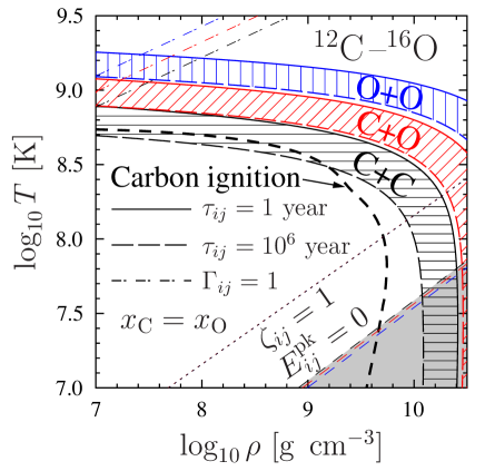
Figure 1: (Color online) Temperature-density diagram for ¹²C+¹⁶O mixture with equal number densities of ¹²C and ¹⁶O. The dash-dot lines correspond (from top to bottom) to $\Gamma_{\mathrm{OO}}$, $\Gamma_{\mathrm{CO}}$, $\Gamma_{\mathrm{CC}}=1$. For temperatures below these lines, the effects of plasma screening on corresponding reaction rates become strong. The dotted line is $\zeta_{ij}=1$. This line is the same for all $i$ and $j$ because of the same $A/Z=2$ ratio. The reacting nuclei become bound along the dashed straight lines (the Gamow-peak energy passes through zero, see Sec. V). For lower temperatures (gray region) the mean field model (used in this paper) becomes inadequate. The shaded regions are bound by solid and long-dashed lines of constant burning times ($1$ yr and $10^{6}$ yr). The thick dash line is the carbon ignition curve (Sec. VI).

Figure 1 is the temperature-density diagram for a ¹²C+¹⁶O mixture with equal number densities of both species. Also, we present the lines of constant dimensionless parameters (see Sec. II.2) $\Gamma_{ij}=1$ (dash-dot lines) and $\zeta_{ij}=1$ (the dotted line). The dash-dot lines (from top to bottom) correspond to $\Gamma_{\mathrm{OO}}=1$, $\Gamma_{\mathrm{CO}}=1$, and $\Gamma_{\mathrm{CC}}=1$. The $\zeta_{ij}=1$ line is the same for all combinations of ions because of equal $A/Z=2$ rations for ¹²C and ¹⁶O ions. The shaded regions are bounded by the solid and long-dashed lines of constant burning times of $1$ and $10^{6}$ yr, respectively. The region for the O+O reaction is highest, for C+O intermediate, and for C+C lowest (as regulated by the height of the Coulomb barrier). The lines of constant burning time are similar. At $\rho\lesssim 10^{9}$ g cm^-3 they mainly depend on temperature because of exponentially strong temperature dependence of the reaction rates. These parts of the lines correspond to thermonuclear burning (with weak or strong plasma screening). With growing density, the curves bend and become nearly vertical (that corresponds to the pycnonuclear burning due to zero-point vibrations of atomic nuclei; see svh69 ; vhs67 ; sk90 ; YGABW06 ). The pycnonuclear reaction rate is a rapidly varying function of density, which is either slightly dependent or almost independent of temperature.

The carbon ignition curve (discussed in Sec. VI) is shown by the thick dashed line.

II.2 Dimensionless parameters

Let us consider a binary mixture of ions with mass numbers $A_{1}$ and $A_{2}$, charge numbers $Z_{1}$ and $Z_{2}$, and fractional numbers $x_{1}=n_{1}/n_{\mathrm{i}}$ and $x_{2}=1-x_{1}$. Following Itoh et al. ikm90 , in addition to the ion radii $a_{i}=a_{ii}$ we introduce an effective radius

$$a_{12}=\frac{a_{1}+a_{2}}{2}=\frac{Z_{1}^{1/3}+Z_{2}^{1/3}}{2}\,a_{\mathrm{e}}$$ (5)

It is also convenient to define the parameter

$$\Gamma_{\mathrm{e}}=e^{2}/(a_{\mathrm{e}}\,k_{\mathrm{B}}\,T),$$ (6)

The coupling parameters for ions can be written as

$$\Gamma_{i}=\Gamma_{ii}=\Gamma_{\mathrm{e}}\,Z_{i}^{5/3}.$$ (7)

In addition, we introduce an effective Coulomb coupling parameter

$$\Gamma_{\mathrm{12}}=Z_{1}Z_{2}e^{2}/(a_{12}k_{\mathrm{B}}\,T),$$ (8)

to be used later for studying a reaction of the type $(A_{1},Z_{1})+(A_{2},Z_{2})$.

Furthermore, we introduce the corresponding ion radius and the Coulomb coupling parameter for a compound nucleus $(A_{i}+A_{j},Z_{i}+Z_{j})=(A_{ij}^{\mathrm{comp}},Z_{ij}^{\mathrm{comp}})$,

$$a^{\mathrm{comp}}_{ij}=a_{\mathrm{e}}\,\left(Z^{\mathrm{comp}}_{ij}\right)^{1/3},\quad\Gamma^{\mathrm{comp}}_{ij}=\Gamma_{\mathrm{e}}\left(Z^{\mathrm{comp}}_{ij}\right)^{5/3}.$$ (9)

The Coulomb barrier penetrability in the classical thermonuclear regime (neglecting plasma screening) is characterized by the parameter

$$\tau_{ij}=\left(\frac{27\pi^{2}\mu_{ij}Z_{i}^{2}Z_{j}^{2}e^{4}}{2k_{\mathrm{B}}T\hbar^{2}}\right)^{1/3}.$$ (10)

The Gamow peak energy in this regime is

$$E_{ij}^{\mathrm{pk}}=k_{\mathrm{B}}T\,\tau_{ij}/3.$$ (11)

The effects of plasma screening on the Gamow peak energy and tunneling range are discussed in Sec. V.

Also, we introduce a dimensionless parameter

$$\zeta_{ij}=3\,\Gamma_{ij}/\tau_{ij}.$$ (12)

In an OCP, $\zeta_{ii}$ reduces to the parameter $\zeta$ defined in Ref. OCP_react and has a simple meaning – it is the ratio of the tunneling length of nuclei with the Gamow peak energy (calculated neglecting of the plasma screening effects) to the ion sphere radius $a_{ij}$.

III Mean field potential

Direct calculation of the contact probability $g_{ij}(0)$ is very complicated even in OCP. In principle, it can be done by Path Integral Monte Carlo (PIMC) simulations, but it requires very large computer resources. PIMC calculations performed so far are limited to a small number of plasma ions (current OCP results are described in ogata97 ; pm04 ; mp05 ). In BIMs one needs a larger number of ions, $N_{1}$ and $N_{2}$, to get good accuracy.

We will use a simple mean-field model, summarized in this section. It can be treated as a first approximation to the PIMC approach aj78 . Previously we showed OCP_react it is in good agreement with PIMC calculations of Militzer and Pollock mp05 for OCP.

A classical pair correlation function, calculated by the classical Monte Carlo (MC) method, can be presented as

$$g^{\mathrm{MC}}_{ij}(r)=\exp\left[\frac{1}{k_{\mathrm{B}}T}\,\left(\frac{Z_{i}Z_{j}e^{2}}{r}-H_{ij}(r)\right)\right],$$ (13)

where $H_{ij}(r)$ is the mean field potential to be determined.

The Taylor expansion of $H_{ij}(r)$ in terms of $r$ for a strongly coupled ion system should contain only even powers widom63 . The first two terms can be derived analytically in the same technique as proposed by Jancovici jancovici77 for OCP. The mean field potential at low $r\ll a_{ij}$ takes form oii91

$$H_{ij}(r)\approx\,k_{\mathrm{B}}Th_{ij}^{0}-\frac{Z_{i}Z_{j}e^{2}}{2a^{\mathrm{comp}}_{ij}}\left(\frac{r}{a^{\mathrm{comp}}_{ij}}\right)^{2},$$ (14)

where

$$h_{ij}^{0}=f_{0}(\Gamma_{i})+f_{0}(\Gamma_{j})-f_{0}(\Gamma_{ij}^{\mathrm{comp}}),$$ (15)

and $f_{0}(\Gamma)$ is the Coulomb free energy per ion in OCP. Here, the linear mixing rule is assumed. In principle, $h_{ij}^{0}$ can be extrapolated from MC $H_{ij}(r)$ data (e.g., Ref. ds99 ), but the problem is delicate rosenfeld96 and we expect that using linear mixing rule is preferable. The linear mixing rule is confirmed with high accuracy dsc96 ; ds03 but its uncertainties were a subject of debates; see Ref. Potekhin_Mixt for recent results.

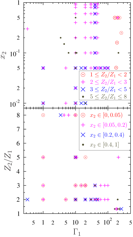
Figure 2: (Color online) Every BIM MC run is shown on both panels. Up: $x_{2}$ versus $\Gamma_{\mathrm{1}}$. Circles, pluses, crosses and dots refer to runs with different ratios of $Z_{2}/Z_{1}$: $1\leq Z_{2}/Z_{1}<2$, $2\leq Z_{2}/Z_{1}<3$, $3\leq Z_{2}/Z_{1}<5$, $5\leq Z_{2}/Z_{1}\leq 8$, respectively. Down: $Z_{2}/Z_{1}$ versus $\Gamma_{\mathrm{1}}$. Circles, pluses, crosses and dots refer to runs with different fractions $x_{2}$: $x_{2}<0.05$, $0.05\leq x_{2}<0.2$, $0.2\leq x_{2}<0.4$, $0.4\leq Z_{2}/Z_{1}\leq 1$.

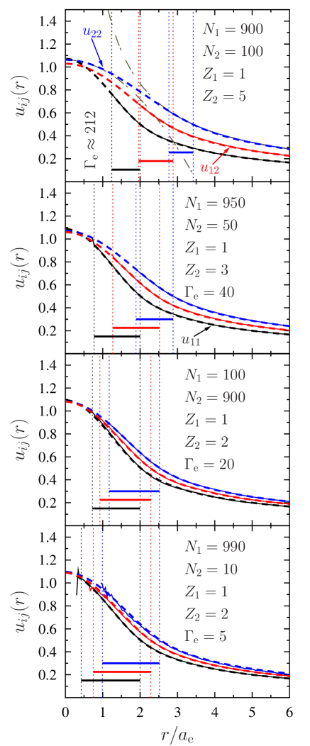
Figure 3: (Color online) Mean field potential $u_{ij}$ versus $r/a_{\mathrm{e}}$ for four MC runs. Solid lines are extracted from MC data, dashed lines are given by the fit (III). On each plot the lines, which are upper at $r\gtrsim 2\,a_{\mathrm{e}}$, correspond to $u_{22}(r)$; lower lines are $u_{12}$ and lowest lines give $u_{11}$. Thin vertical dotted lines connected by thick solid lines show the ranges of $r$, which are used in the fitting.

To determine the mean field potential in BIMs we performed extensive MC calculations of $H_{ij}(r)$. We did 129 MC runs. In each run we calculated pair correlation functions $g_{11}$, $g_{12}$ and $g_{22}$ for a given set of the parameters $Z_{1}$, $Z_{2}$, $N_{1}$, $N_{2}$, and $\Gamma_{1}$. In Fig. 2 each set is shown by a symbol. The top panel demonstrates a fraction of particles 2, $x_{2}$, versus $\Gamma_{1}$. Circles, pluses, crosses and dots refer to different ratios of $Z_{2}/Z_{1}$: $1\leq Z_{2}/Z_{1}<2$, $2\leq Z_{2}/Z_{1}<3$, $3\leq Z_{2}/Z_{1}<5$, $5\leq Z_{2}/Z_{1}\leq 8$, respectively. In the bottom panel we show the $Z_{2}/Z_{1}$-ratio versus $\Gamma_{1}$. Circles, pluses, crosses and dots correspond to different values of $x_{2}$: $x_{2}<0.05$, $0.05\leq x_{2}<0.2$, $0.2\leq x_{2}<0.4$, $0.4\leq x_{2}\leq 1$. For some parameter sets (e.g., for $\Gamma_{1}=180$, $x_{2}\approx 0.05$, $Z_{2}/Z_{1}=4/3$) we use a number of MC runs with different initial configurations (random or regular lattice) and/or different simulation times. We did not find any significant dependence of the mean field potential (for $r<2a_{ij}$) on the initial parameters. From all our simulations we extract $H_{11}(r)$, $H_{12}(r)$ and $H_{22}(r)$ and remove some low-$r$ points with large MC noise. We then fit these functions at $r\lesssim 2a_{ij}$ by a simple universal analytical expression

$$H_{ij}(r) = k_{\mathrm{B}}T\,\Gamma_{ij}^{\mathrm{eff}}$$

$$\times \sqrt{\frac{U_{0}^{2}+U_{1}\,x^{4}+U_{2}\,x^{8}}{1+U_{3}\,x+U_{4}\,x^{2}+U_{5}\,x^{4}+U_{6}\,x^{6}+U_{2}\,x^{10}}},$$

where $x=r/a^{\mathrm{eff}}_{ij}$, $U_{0}=h_{ij}^{0}/\Gamma^{\mathrm{eff}}_{ij}$, $U_{1}=0.0319$, $U_{2}=0.0024$, $U_{3}=0.22\left(\Gamma^{\mathrm{eff}}_{ij}\right)^{-0.7}$, $U_{4}=2^{-1/3}\left(a^{\mathrm{eff}}_{ij}/a^{\mathrm{comp}}_{ij}\right)^{2}/U_{0}$, $U_{5}=0.111$, and $U_{6}=0.0305$. Note, that $U_{0}$ and $U_{4}$ are fixed by the low-$r$ asymptote of $H_{ij}(r)$ at strong Coulomb coupling, $\Gamma_{ij}\gg 1$, Eq. (14). For a better determination of $H_{12}(r)$, we introduce the effective ion sphere radius $a^{\mathrm{eff}}_{ij}$ and the Coulomb coupling parameter $\Gamma^{\mathrm{eff}}_{ij}$:

$$a^{\mathrm{eff}}_{ij}=\left(\frac{a_{i}^{p}+a_{j}^{p}}{2}\right)^{1/p},\quad\Gamma^{\mathrm{eff}}_{ij}=\frac{Z_{i}Z_{j}e^{2}}{k_{\mathrm{B}}Ta^{\mathrm{eff}}_{ij}}.$$ (17)

Here, $p$ is an additional fit parameter which is found to be $p=1.6$. Note, that $a^{\mathrm{eff}}_{ii}=a_{ii}=a_{i}$ for reactions with identical nuclei ($i=j$). If, however, $i\neq j$ the parameters $a^{\mathrm{eff}}_{ij}$ and $a_{ij}$ differ by a few percent and this difference is very important. Using $a_{ij}$ to define $x$ in Eq. (III) and using $H_{ij}(r)$ to reproduce the pair correlation function $g_{ij}(r)$ through Eq. (13), we find the first peak of $g_{ij}$ to be unrealistically deformed for large $Z_{2}/Z_{1}\gtrsim 5$.

Let us mention that in the OCP case our fit expression (III) is not the same as we used previously OCP_react . Equation (III) seems to be better because it better describes the first peak of $g(r)=g_{ii}(r)$, especially at very large $\Gamma\gtrsim 200$. For an OCP at $\Gamma\lesssim 200$, the old and new fit expressions give approximately the same accuracy of $H(r)=H_{ii}(r)$.

Four examples of MC runs are shown in Fig. 3. For each run (on each plot) we show dimensionless mean field potential $u_{ij}=H_{ij}(r)/(k_{\mathrm{B}}T\Gamma_{ij})$ versus $r/a_{\mathrm{e}}$. Solid lines are MC data, dashed lines are derived from the fit expression (III). One can see numerical noise of MC data at low $r$; it is especially strong in the lowest plot for $\Gamma_{\mathrm{e}}=5$. During fitting procedure we removed some low-$r$ points with high MC noise. Our fitting ranges are shown by pairs of thin dotted lines connected by a thick solid line. The low-$r$ bound of the fitting region is different for $H_{11}$, $H_{12}$, and $H_{22}$ and for each MC run. The high-$r$ bound was taken to be $2a_{ij}$ for all data. Thus, all our fits include the vicinity of the first peak of a pair correlation function at $r\sim 1.8a_{ij}$. Although we have no MC data at low $r$, we expect that our approximation is well established because it satisfies the accurate low-$r$ asymptote (14). Also, it satisfies the large-$r$ asymptote $u_{ij}(r\rightarrow 1)=a_{ij}/r$, which corresponds to the fully screened Coulomb potential. Both asymptotes for $u_{22}$ are shown on the upper plot by dash-dot lines. One can see, that they nicely constrain the mean field potential.

A poor MC statistics at low $r$ can be, in principle, increased using specific MC schemes cg03 but this is beyond the scope of the present paper.

Previously the mean field approximations was used by Itoh et al. ikm90 and Ogata et al. oiv93 . While we use the correct form of the linear mixing rule (15) to calculate $u_{12}(0)$, the cited authors restricted themselves by OCP results, which depend only on $\Gamma_{12}$ (but not on $Z_{2}/Z_{1}$). The results of this simplification are discussed in Sec. IV; they are visible in Fig. 4. In addition, our approximation is based on a more representative set of MC runs (see Fig. 2), and each run was done with better accuracy. For example, where is no visible noise $g_{ij}(r)$-noise in the vicinity of the first peak in out data, whereas this noise is obvious in Fig. 1 of Ref. oiv93 . We have also checked that our approximation (III) better reproduces all our MC data than approximations of both groups ikm90 ; oiv93 . As noted by Ogata et al. oiv93 , the height of the first $g_{ij}(r)$-peak depends on the fraction of ions with larger charge (the peaks become higher with increasing this fraction). Our data confirm this statement for a not very large Coulomb coupling parameter, $\Gamma_{1}\lesssim 10$. Ogata et al. oiv93 added a correction for this feature in their approximation of $u_{11}$. It helps to describe the first $g_{11}(r)$-peak for some of our runs (e.g., for $\Gamma_{1}=10$, $Z_{2}/Z_{1}=5$ and $x_{2}=0.2$). However, we think that we still do not have enough data to quantitatively describe this correction to the linear mixing with good accuracy, and we use the mean field potential (III) based on the linear mixing rule throughout the paper. In the Appendix we describe the corrections to the linear mixing on a phenomenological level.

IV Enhancement of nuclear reaction rates

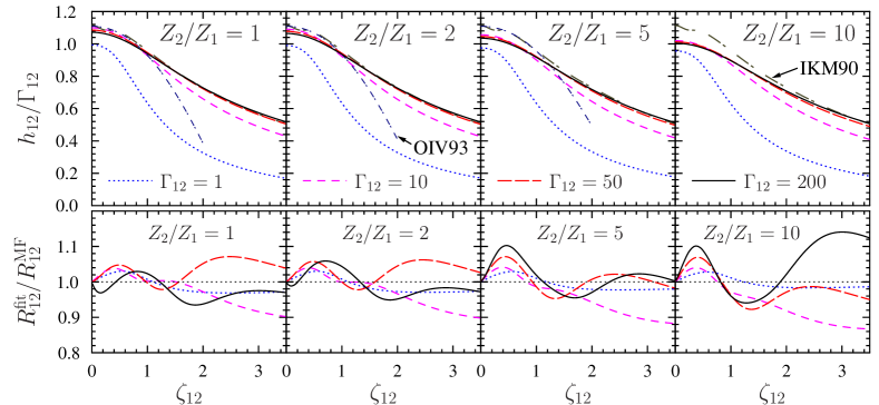
Figure 4: (Color online) Top: Enhancement factors $h_{ij}/\Gamma_{12}$ for several $\Gamma_{12}$ (=1, 10, 50, 200; each shown by a line on every panel) and $Z_{2}/Z_{1}$ (=1, 2, 5, 10; each on its own panel). The long dash-dot line presents the fit expression by Itoh et al. ikm90 (IKM90); the short dash-dot lines are the results by Ogata et al. oiv93 (OIV93), calculated for $\Gamma_{12}=50$, as an example (the latter lines are shown only for $\zeta_{12}<2$ and $Z_{2}/Z_{1}\leq 5$ which are the fit bounds in OIV93). Bottom: Ratios of $R_{12}^{\mathrm{fit}}$, given by Eq. (23), to the mean field reaction rate $R_{12}^{\mathrm{MF}}$, given by (20), versus $\zeta_{12}$. See text for details.

Let us introduce the enhancement factor $F^{\mathrm{scr}}_{ij}$ of a nuclear reaction rate $R^{\mathrm{scr}}_{ij}$ under the effect of plasma screening,

$$R^{\mathrm{scr}}_{ij}=R^{\mathrm{th}}_{ij}\,F^{\mathrm{scr}}_{ij},\quad F^{\mathrm{scr}}_{ij}=\exp(h_{ij}).$$ (18)

Here, $R^{\mathrm{th}}_{ij}$ is the reaction rate in the absence of the screening. In can be calculated using the classical theory of thermonuclear burning,

$$R^{\mathrm{th}}_{ij}=\frac{4n_{i}n_{j}}{1+\delta_{ij}}\,\frac{S_{ij}(E^{\mathrm{pk}}_{ij})}{k_{\mathrm{B}}T}\,\sqrt{\frac{2E^{\mathrm{pk}}_{ij}}{3\mu_{ij}}}\exp\left(-\tau_{ij}\right).$$ (19)

The barrier penetrability parameter $\tau_{ij}$ and the Gamow peak energy $E^{\mathrm{pk}}_{ij}$, which enter this equation, are defined, respectively, by Eqs. (10) and (11).

Using $H_{ij}(r)$ we can calculate the reaction rate. This calculation takes into account the plasma screening enhancement in the mean-field approximation (as was done for OCP in our previous paper OCP_react ),

$$R^{\mathrm{MF}}_{ij} = \frac{n_{i}\,n_{j}S_{ij}\left({E^{\mathrm{pk}}_{ij}}^{\prime}\right)}{1+\delta_{ij}}\,\sqrt{8\over\pi\mu_{ij}(k_{\mathrm{B}}T)^{3}}\,$$ (20)

$$\times\int_{E_{\mathrm{min}}}^{\infty}{\rm d}E\,\exp\left[-\frac{E}{k_{\mathrm{B}}T}-P_{ij}(E)\right].$$

Here, $E$ is the center-of-mass energy of the colliding nuclei (with a minimum value $E_{\mathrm{min}}$ at the bottom of the potential well), $\exp(-E/k_{\mathrm{B}}T)$ comes from the Maxwellian energy distribution of the nuclei, and

$$P_{ij}(E)={2\sqrt{2\mu_{ij}}\over\hbar}\,\int_{0}^{r_{t}}{\rm d}r\,\sqrt{{Z_{i}Z_{j}e^{2}\over r}-H_{ij}(r)-E}$$ (21)

is the Coulomb barrier penetrability ($r_{t}$ being a classical turning point).

In the WKB mean-field approximation the enhancement factor of the nuclear reaction rate is

$$F^{\mathrm{scr}}_{ij}=R^{\mathrm{MF}}_{ij}\{H_{ij}\}/R^{\mathrm{MF}}_{ij}\{H_{ij}=0\}.$$ (22)

In the cases of physical interest, $R^{\mathrm{MF}}_{ij}\{0\}$ can be integrated by the saddle-point method. However, we always integrate in Eq. (20) numerically.

The calculated enhancement factor $F^{\mathrm{scr}}_{ij}$ can be fitted as

$$\log F^{\mathrm{scr}}_{ij}=f_{0}\left(\frac{\Gamma_{i}}{\tau_{ij}}\right)+f_{0}\left(\frac{\Gamma_{j}}{\tau_{ij}}\right)-f_{0}\left(\frac{\Gamma_{ij}^{\mathrm{comp}}}{\tau_{ij}}\right),$$ (23)

where $f_{0}(\Gamma)$ is a free energy per ion in an OCP. We use the most accurate available analytic fit for $f_{0}(\Gamma)$ suggested by Potekhin and Chabrier pc00 :

$$f_{0}(\Gamma) = A_{1}\left[\sqrt{\Gamma\,\left(A_{2}+\Gamma\right)}\right.$$ (24)

$$- \left.A_{2}\ln\left(\sqrt{\Gamma/A_{2}}+\sqrt{1+\Gamma/A_{2}}\right)\right]$$

$$+ 2A_{3}\left[\sqrt{\Gamma}-\arctan\left(\sqrt{\Gamma}\right)\right]$$

$$+ B_{1}\left[\Gamma-B_{2}\ln\left(1+\frac{\Gamma}{B_{2}}\right)\right]$$

$$+ \frac{B_{3}}{2}\ln\left(1+\frac{\Gamma^{2}}{B_{4}}\right).$$

Here, $A_{1}=-0.907$, $A_{2}=0.62954$, $A_{3}=-\sqrt{3}/2-A_{1}/\sqrt{A_{2}}\approx 0.2771$, $B_{1}=0.00456$, $B_{2}=211.6$, $B_{3}=-10^{-4}$, $B_{4}=0.00462$. We also introduce a number of additional parameters:

$$y_{ij} = \frac{4\,Z_{i}\,Z_{j}}{\left(Z_{i}+Z_{j}\right)^{2}},\quad c_{1}=0.013\,y_{ij}^{2},$$

$$c_{2} = 0.406\,y_{ij}^{0.14},\quad c_{3}=0.062\,y_{ij}^{0.19}+1.8/\Gamma_{ij},$$

$$t_{ij} = \left(1+c_{1}\,\zeta_{ij}+c_{2}\,\zeta_{ij}^{2}+c_{3}\zeta_{ij}^{3}\right)^{1/3}.$$ (25)

The root-mean-squared relative error of the fit of $F_{\mathrm{scr}}$ is $5\%$. The maximum error $\sim 14\%$ occurs at $\zeta_{ij}\approx 4.8$, $\Gamma_{12}\approx 25$, and $Z_{2}/Z_{1}\approx 10$. The fit was constructed for $1\leq Z_{2}/Z_{1}\leq 10$, $1\leq\Gamma_{12}\leq 200$ (we also use $\Gamma_{12}=400$ and $600$ for testing) and $\zeta_{12}\leq 8$ (larger values of $\zeta_{12}$ were not included into fitting but used for tests). As for OCP in our previous paper OCP_react , at larger $\Gamma$ the relative errors increase.

In the limit of $\zeta_{ij}\rightarrow 0$ we have $\log F^{\mathrm{scr}}_{ij}=h_{ij}^{0}$. This is the well known relation (e.g., salpeter54 ; dgc73 ); its formal proof is given in ys89 .

Our fit formula (23) has the same form as the thermodynamic relation (15), but contains Coulomb coupling parameters $\Gamma_{ij}$ divided by $\tau_{ij}$. It generalizes our OCP result OCP_react .

Figure 4 shows the normalized enhancement factor $h_{12}/\Gamma_{12}$ (bottom panels) as a function of $\zeta_{12}$ for several values of $\Gamma_{12}$ ($=1$, $10$, $50$, $200$; separate lines on each plot) and $Z_{2}/Z_{1}$ ($=1$, $2$, $5$ and $10$, separate plots). The first panel (for $Z_{2}=Z_{1}$) corresponds not only to a reaction in OCP, but to reactions of identical nuclei in a mixture; the mean field potential and the plasma screening enhancement do not depend on an admixture of other elements [see Eqs. (III) and (23)], as long as the Coulomb coupling parameter is not too small, $\Gamma_{ij}\gtrsim 1$, and the linear mixing is valid. The larger $\Gamma_{ij}$, the weaker is the dependence of $h_{12}/\Gamma_{12}$ on $\Gamma_{ij}$. Long-dashed lines, plotted for $\Gamma_{12}=50$, significantly differ from dashed lines which are for $\Gamma_{12}=10$, but can be hardly distinguished from solid lines, plotted for $\Gamma_{12}=200$. Therefore, the total enhancement factor $\exp\left(h_{12}\right)$ depends exponentially on $\Gamma_{12}$ in the first approximation. The normalized enhancement factor $h_{12}/\Gamma_{12}$ suggested by Itoh et al. ikm90 (IKM90) is shown by long dash-dot lines. It is independent of $\Gamma_{12}$, and we show one line in each plot. The short dash-dot lines demonstrate the fit expression of Ogata et al. oiv93 (OIV93) (for $\Gamma_{12}=50$ as an example). The lines are cut at $\zeta_{12}=2$ (that bounds the fit validity). We show no OIV93 line on the panel for $Z_{2}/Z_{1}=10$ because there are no OIV93 simulations for such large $Z_{2}/Z_{1}$ ratios. The two lines, IKM90 and OIV93, demonstrate higher enhancement, especially for $\zeta_{12}\lesssim 1$ and large $Z_{2}/Z_{1}$. First, IKM90 and OIV93 used less accurate thermodynamic approximations for calculating $u_{ij}(0)$. For large $Z_{2}/Z_{1}$-ratios, their fit error increases because of using the OCP expression (dependent only of $\Gamma_{12}$, but not on $Z_{2}/Z_{1}$) for determining $u_{ij}(0)$. This increases a difference between our and their approximations at large $Z_{2}/Z_{1}$ (see also a discussion in Sec. IIIC of Ref. YGABW06 ). IKM90 and our $\zeta_{12}$-dependence of the enhancement factors is qualitatively the same, but the results of OIV93 (and of the preceding paper oii91 ) are qualitatively different. As we show previously OCP_react , such results contradict recent PIMC results by Militzer and Pollock mp05 for OCP. The deviation of the IKM90 enhancement factors at low $\zeta_{ij}$ values comes possibly from using an oversimplified mean field potential.

The indicated differences between IKM90, OIV93 and our results can lead to very large differences of the total enhancement factor $\exp\left(h_{12}\right)$. For example, at $Z_{2}/Z_{1}=5$ and $\Gamma_{12}=200$ the difference can reach five orders of magnitude. Accordingly, we do not present the IKM90 and OIV93 results in lower panels, which give the ratio of the reaction rates $R^{\mathrm{fit}}_{12}$, given by the fit expression (23), to the reaction rate $R^{\mathrm{MF}}_{12}$, calculated in the mean field approximation using Eq. (20). A very small difference ($\lesssim 10\%$), shown on these plots, is true only by adopting the mean field potential (III). The uncertainties of the reaction rates, which come from the uncertainties of the mean field potential and inaccuracy of the mean field approximation, can be larger.

Let us stress that Eq. (23) is derived for the case of strong screening; it is invalid at $\Gamma_{12}\lesssim 1$, where the adopted linear mixing rule fails. A simple correction of the enhancement factor for weaker screening is suggested in the Appendix. It allows us to extend the results for the case of weaker Coulomb coupling.

V Astrophysical S-factors: Gamow peak energies at strong screening

In the previous section we focused on the plasma screening of the Coulomb barrier penetration in dense plasma environment. Now we discuss the effects of plasma screening on the astrophysical $S$-factor, that describes nuclear interaction of the reacting nuclei after the Coulomb barrier penetration. The latter effects are not expected to be very strong because of not too strong energy dependence of $S_{ij}(E)$ (e.g., Ref. Gasetal07 ), but we consider them for completeness.

The astrophysical $S$-factor describes the effects of short-range nuclear forces and it should depend on the parameters of the reacting nuclei just before a reaction event. The energy ${E^{\mathrm{pk}}_{ij}}^{\prime}$ substituted into $S(E)$ in Eq. (20) should be corrected for the mean field potential created by other ions, ${E^{\mathrm{pk}}_{ij}}^{\prime}=E+H_{ij}(0)$. This correction is obvious and has been used in calculations (e.g., itw03 ), but its formal proof has not been published, to the best of our knowledge. The reaction rate in the presence of plasma screening can be calculated as

$$R_{ij} = \frac{n_{i}n_{j}}{1+\delta_{ij}}\left(\frac{8}{\pi\mu_{ij}T^{3}}\right)^{1/2}$$ (26)

$$\times \int\widetilde{\sigma}_{ij}(E)E\exp\left(-\frac{E}{T}\right)\mathrm{d}E,$$

where $\widetilde{\sigma}_{ij}(E)$ is the reaction cross section including the screening effects. To calculate $R_{ij}$, let us remind the barrier penetration model a with parameter-free model of nuclear interaction gives a good description of reaction cross sections Gasques_etal05 . In the absence of plasma screening at not too high energies $E$ (where only the s-wave channel is important), this model reduces to the WKB calculation of the penetrability through a potential which is the sum of the Coulomb potential and the potential $V^{\mathrm{N}}_{ij}(r,v_{ij}^{2})$, that describes the short-range nuclear interaction. The latter potential depends on the local relative velocity $v(r.E)$ of the reactants given by

$$v^{2}=\frac{2}{\mu_{ij}}\left[E+H_{ij}(r)-\frac{Z_{i}Z_{j}e^{2}}{r}-V^{\mathrm{N}}_{ij}(r,v^{2})\right].$$ (27)

Let us generalize this model by adding the screening potential $H_{ij}(r)$ and write the cross section as

$$\widetilde{\sigma}_{ij}(E) = \frac{\pi}{k_{ij}^{2}}\exp\left[-\frac{2\sqrt{2\mu_{ij}}}{\hbar}\int_{r_{\mathrm{tn}}}^{r_{\mathrm{t}}}\mathrm{d}r\right.$$ (28)

$$\times \left.\sqrt{\frac{Z_{i}Z_{j}e^{2}}{r}-H_{ij}(r)+V^{\mathrm{N}}_{ij}(r,v_{ij}^{2})-E}\right].$$

Here, $r_{\mathrm{tn}}$ and $r_{\mathrm{t}}$ are classical turning points and $k_{ij}^{2}=2\mu_{ij}E/\hbar^{2}$. Substituting this equation into Eq. (26) we have

$$R = \frac{n_{i}n_{j}}{1+\delta_{ij}}\left(\frac{8}{\pi\mu_{ij}T^{3}}\right)^{1/2}$$ (29)

$$\times \int\widetilde{S}_{ij}(E)\exp\left[-\frac{E}{T}-P_{ij}(E)\right]\mathrm{d}E,$$

where $\widetilde{S}_{ij}(E)$ is the astrophysical factor, calculated in the presence of the plasma screening,

$$\widetilde{S}_{ij}(E)=\widetilde{\sigma}_{ij}E\exp\left[P_{ij}(E)\right];$$ (30)

$P_{ij}(E)$ is defined by Eq. (21). The potential $V^{\mathrm{N}}_{ij}(r,v)$ is non-zero only for very small $r\lesssim r_{\mathrm{N}}$. Let us substitute Eqs. (21) and (28) into (30) and divide all integrals into two parts, at $r<r_{\mathrm{N}}$ and $r\geq r_{\mathrm{N}}$. The integrals over $r>r_{\mathrm{N}}$ which come from $P_{ij}(E)$ and $\widetilde{\sigma}_{ij}(E)$ will be exactly the same ($V^{\mathrm{N}}_{ij}(r,v)=0$ for $r>r_{\mathrm{N}}$) and cancel each other. As a result,

$$\widetilde{S}_{ij}(E) = \frac{\pi\hbar^{2}}{2\mu_{ij}}\exp\left\{\frac{2\sqrt{2\mu_{ij}}}{\hbar}\right.$$

$$\times \left[\int_{0}^{r_{\mathrm{N}}}\sqrt{\frac{Z_{i}Z_{j}e^{2}}{r}-H_{ij}(r)-E}\,\mathrm{d}r\right.$$

$$- \left.\left.\int_{r_{\mathrm{tn}}}^{r_{\mathrm{N}}}\sqrt{\frac{Z_{i}Z_{j}e^{2}}{r}-H_{ij}(r)+V^{\mathrm{N}}_{ij}(r,v^{2})-E}\,\mathrm{d}r\right]\right\}.$$

As expected, the astrophysical $S$-factor is determined by the behavior of the total potential $Z_{i}Z_{j}e^{2}/r-H_{ij}(r)+V^{\mathrm{N}}_{ij}(r,v^{2})$ in the low-$r$ region $r<r_{\mathrm{N}}$, where the nuclear forces are important. Because $r_{\mathrm{N}}$ is much smaller than the ion sphere radius $a_{ij}$, which is a typical length scale of $H_{ij}(r)$ (e.g., Fig. 3), we can neglect variations of $H_{ij}(r)$ for $r<r_{\mathrm{N}}$ and replace $H_{ij}(r)$ under the integrals in Eq. (V) by $H_{ij}(0)$. The $S_{ij}(E)$-factor in the absence of plasma screening is given by the same Eq. (V) but at $H_{ij}(r)=0$. Thus, $\widetilde{S}_{ij}(E)$ is defined by the same equation as $S_{ij}(E^{\prime})$, provided $E^{\prime}=E+H_{ij}(0)$. In other words, $\widetilde{S}_{ij}(E)=S_{ij}(E+H_{ij}(0))$ and the reaction rate is

$$R = \frac{n_{i}n_{j}}{1+\delta_{ij}}\left(\frac{8}{\pi\mu_{ij}k_{\mathrm{B}}^{3}T^{3}}\right)^{1/2}$$ (32)

$$\times \int S_{ij}(E+H_{ij}(0))\exp\left[-\frac{E}{k_{\mathrm{B}}T}-P_{ij}(E)\right]\mathrm{d}E.$$

If this simple barrier penetration theory were invalid and the hypothesis of low-energy hindrance of nuclear reactions jiangetal07 were correct, such a simple correction of astrophysical $S$-factors for the plasma screening effects could be insufficient, and the calculation of the reaction rate would be much more complicated. We will not consider this possibility.

As in of the absence of the plasma screening, the main contribution to the integral (32) comes from a narrow energy range. We neglect the energy dependence of $S_{ij}(E+H_{ij}(0))$ in this range and take the $S$-factor out of the integral. The contact probability in the mean field model is given by

$$g_{ij}(0)=\frac{2\sqrt{2\pi\mu_{ij}}}{k_{\mathrm{B}}^{3/2}T^{3/2}}\frac{Z_{1}\,Z_{2}e^{2}}{\hbar}\int\exp\left[-\frac{E}{k_{\mathrm{B}}T}-P_{ij}(E)\right]\mathrm{d}E,$$ (33)

so that the reaction rate reads

$$R_{ij}=\frac{2\,n_{i}n_{j}}{1+\delta_{ij}}\frac{a^{\mathrm{B}}_{ij}}{\hbar\pi}S_{ij}\left(E^{\mathrm{pk}}_{ij}+H_{ij}(0)\right)g_{ij}(0).$$ (34)

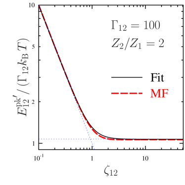
Figure 5: (Color online) The Gamow peak energy ${E^{\mathrm{pk}}_{ij}}^{\prime}$ normalized for $\Gamma_{12}$ as function of $\zeta_{12}$ at $Z_{2}/Z_{1}=2$ and $\Gamma_{12}=100$. Solid line is the fit expression (35), dashed line shows the mean field result. Thin dotted lines correspond to the low-$\zeta_{ij}$ thermonuclear asymptote ${E^{\mathrm{pk}}_{ij}}^{\prime}=\Gamma_{12}/\zeta_{12}$ and high-$\zeta_{ij}$ pycnonuclear asymptote ${E^{\mathrm{pk}}_{ij}}^{\prime}=H_{ij}(0)$. See text for details.

We have calculated the modified Gamow-peak energy ${E^{\mathrm{pk}}_{ij}}^{\prime}=E^{\mathrm{pk}}_{ij}+H_{ij}(0)$, which should be used as an argument of $S$-factors, in a wide range of plasma parameters. It can be fitted as

$${E^{\mathrm{pk}}_{ij}}^{\prime}=\left[H_{ij}^{3}(0)+\left(k_{\mathrm{B}}T\,\frac{\Gamma_{ij}}{\zeta_{ij}}\right)^{3}\right]^{1/3}.$$ (35)

The maximum relative fit error for $1\leq\Gamma_{ij}\leq 200$, $\zeta_{ij}\leq 8$ and $0.1\leq Z_{i}/Z_{j}\leq 10$ is 4%. It takes place at $\Gamma_{ij}=1$, $\zeta_{ij}=1$ and $Z_{i}=Z_{j}$. Because of large nuclear physics uncertainties in our knowledge of $S(E)$ at low energies of astrophysical interest, this accuracy is more than sufficient. An example of the dependence of ${E^{\mathrm{pk}}_{12}}^{\prime}/\Gamma_{12}$ on $\zeta_{12}$ is shown in Fig. 5 for $Z_{2}/Z_{1}=2$ and $\Gamma_{12}=100$. The solid line is the fit (35), the dashed line is a result of the exact ${E^{\mathrm{pk}}_{ij}}^{\prime}$ calculation in the mean field model. The peak energy ${E^{\mathrm{pk}}_{ij}}^{\prime}$ has two asymptotes shown by thin dotted lines. At low $\zeta\ll 1$, the reaction occurs in the thermonuclear regime, ${E^{\mathrm{pk}}_{ij}}^{\prime}=\Gamma_{ij}/\zeta_{ij}$, which is the standard classical result. For large $\zeta_{ij}\gg 1$, we have ${E^{\mathrm{pk}}_{ij}}^{\prime}\to H_{ij}(0)$. The classical asymptote ${E^{\mathrm{pk}}_{ij}}^{\prime}=\Gamma_{ij}/\zeta_{ij}$ is applicable at $\zeta_{ij}\lesssim 0.5$, where the plasma screening enhancement can be very strong (tenths orders of magnitude). This is because in the thermonuclear regime the tunneling length is not very large and $H_{ij}(r)$ does not significantly change it (see Fig. 6); ions tunnel through the Coulomb potential, shifted by $H_{ij}(0)$. The shift increases the probability of close ions collisions by a factor of $\exp\left(H_{ij}(0)/T\right)$, but does not change the Maxwellian energy distribution and the dependence of the tunneling probability on tunneling length. As a result, the main contribution to the reaction rate comes from ions with the same tunneling length (and the same ${E^{\mathrm{pk}}_{ij}}^{\prime}$), as in the absence of plasma screening.

The large-$\zeta_{ij}$ asymptote is simple. For such parameters, thermal effects are small and the ions, which mainly contribute to the reaction rate, correspond to the minimum energy of the total potential $Z_{1}Z_{2}/r+H_{ij}(r)$. This energy is small compared with $H_{ij}(0)$, so that ${E^{\mathrm{pk}}_{ij}}^{\prime}\approx H_{ij}(0)$. One can see a small difference of $H_{ij}(0)$, shown by the thin dotted line in Fig. 5, and the asymptote of $H_{ij}(0)$ at large $\zeta_{ij}$. This difference does not introduce significant uncertainties to the reaction rate because of much larger nuclear-physics uncertainties caused by our poor knowledge of $S(E)$ at low energies (e.g., Ref. YGABW06 ). We assume that the ${E^{\mathrm{pk}}_{ij}}^{\prime}$ approximation (35) is valid (at least qualitatively) not only for thermonuclear burning with strong screening, but also for pycnonuclear burning. In the pycnonyclear regime, the ions occupy their ground states and oscillate near their lattice sites. The reaction rates are determined by zero-point vibrations of the ions. The energy of zero-point vibrations is typically small compared to the minimum energy of the potential $Z_{i}Z_{j}/r+\widetilde{H}_{ij}(\bm{r})$ (the latter is much lower than $\widetilde{H}_{ij}(0)$, where $\widetilde{H}_{ij}(\bm{r})$ is an anisotropic effective potential created by neighboring ions). Therefore, the ions start with a small kinetic energy (the minimum of the $Z_{i}Z_{j}/r+\widetilde{H}_{ij}(\bm{r})$) and tunnel to $r\rightarrow 0$ through the Coulomb potential plus the $\widetilde{H}_{ij}(\bm{r})$. During tunneling, they fall into the potential well $\widetilde{H}_{ij}({\bm{r}})$, and their energy increases by $\widetilde{H}_{ij}(0)$. Therefore, ${E^{\mathrm{pk}}_{ij}}^{\prime}$ should be equal to $\widetilde{H}_{ij}(0)$, but not to energy of zero-point vibrations, as assumed in svh69 ; sk90 ; YGABW06 . Note, that in the relaxed-lattice approximation $\widetilde{H}_{ij}(0)=H_{ij}(0)$ svh69 ; sk90 .

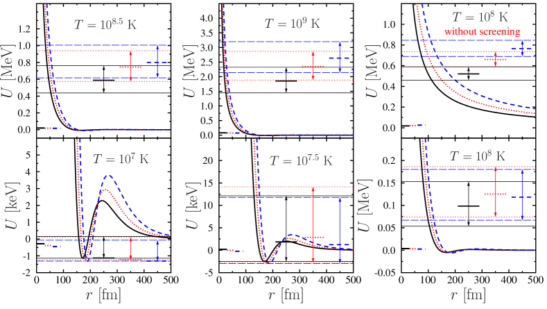
Figure 6: (Color online) Effective mean-field Coulomb potentials $U_{ij}(r)$ for the reactions ${}^{12}\mathrm{C}+^{12}\mathrm{C}$ (solid line), ${}^{12}\mathrm{C}+^{16}\mathrm{O}$ (dotted line) and ${}^{16}\mathrm{O}+^{16}\mathrm{O}$ (long-dash line) in the mixture of ${}^{12}\mathrm{C}$ and${}^{16}\mathrm{O}$ with equal number densities of these nuclei at $\rho=5\times 10^{9}$ g cm^-3 and five temperatures ($\log_{10}T[K]=9$, $8.5$, $8$, $7.5$, and $7$).

For example, let us consider $E^{\mathrm{pk}}_{ij}$ and the characteristic (half-maximum) energy widths of the Gamow peak for a ¹²C and ¹⁶O mixture (with equal number densities of C and O ions) at $\rho=5\times 10^{9}$ g cm^-3. In Fig. 6 we show the effective total radial mean-field Coulomb potentials $U_{ij}(r)=Z_{i}Z_{j}e^{2}/r-H_{ij}(r)$ ($i,j=^{12}$C or ¹⁶O) for five temperatures, $T=10^{9}$, $10^{8.5}$, $10^{8}$, $10^{7.5}$, and $10^{7}$ K. For this mixture, the ion-sphere radius of ¹²C ions is $a_{\mathrm{C}}$=98 fm, and it is $a_{\mathrm{O}}$=108 fm for ¹⁶O ions. The solid, dotted and long-dash lines show the CC, CO and OO potentials, respectively. Each potential $U_{ij}(r)$ has a minimum at $r_{ij}\approx 2a_{ij}$ due to the Coulomb coupling. The thin horizontal lines connected by double-arrow lines in Fig. 6 show the Gamow-peak energy ranges. The types of thin lines are the same as for $U_{ij}(r)$. Thick sections of short horizontal lines, which intersect double-arrow lines, demonstrate the Gamow-peak energies $E^{\mathrm{pk}}_{ij}$. Thick parts of short-dashed lines at small $r<100$ fm indicate the thermal energy level $k_{\mathrm{B}}T$ measured from the bottom of $U_{ij}(r)$.

The top right panel marked “without screening” shows the same lines (as other panels) for $T=10^{8}$ K neglecting plasma screening. Dramatic difference of unscreened and screened potentials and corresponding Gamow-peak regions is obvious from comparison with bottom panels. The plasma screening reduces the Gamow-peak energy $E^{\mathrm{pk}}_{ij}$ by a factor of four, but (as described above) does not affect significantly the Gamow-peak width.

Let us discuss Fig. 6 in more detail. The panels plotted for $T=10^{8.5}$ and $10^{9}$ K (top left and top center, respectively) refer to the thermonuclear reaction regime with strong plasma screening. The next two panels (right bottom and center bottom) are for a colder plasma ($T=10^{8}\mbox{ K}$ and $T=10^{7.5}\mbox{ K}$, respectively), while the last (left bottom) panel is for a very cold plasma ($T=10^{7}\mbox{ K}$) (that is certainly in the zero-temperature pycnonuclear regime). When the temperature decreases, the Gamow-peak energy range becomes thinner (note the difference of energy scales in different panels) and shrinks to lower energies. If $T\gtrsim 10^{8}$ K, the Gamow peak range is still at $E>0$ [belonging to continuum states in a potential $U_{ij}(r)$], and the peak energy $E^{\mathrm{pk}}_{ij}$ (the short-dash horizontal line) is in the center of the Gamow-peak range. The energies within this range are much higher than $k_{\mathrm{B}}T$ supporting the statement that the main contribution to reaction rates at sufficiently high $T$ comes from suprathermal ions. In these cases, the underlying mean-field WKB approximation is expected to be adequate. In the forth panel, the lowest energies of the Gamow-peak range become negative (drop to bound states) and $E^{\mathrm{pk}}_{ij}$ moves from the center to the lower bound of the Gamow-peak range (so that the Gamow peak becomes significantly asymmetric). The mean-field WKB approach based on the spherically symmetric mean field potential $H_{ij}(r)$ may be still qualitatively correct but becomes quantitatively inaccurate. Note that the $U_{ij}(r)$-potential becomes positive for $r\gtrsim 200$ fm. This feature is determined by the right wing of the first $g_{ij}(r)$-peak, where $g_{ij}(r)$ becomes smaller than one. This wing is unimportant in the mean field model; our approximation gives qualitatively correct $U_{ij}(r)$ for $r\gtrsim 2a_{ij}$ ($g_{ij}(r)\rightarrow 1$ for $r\rightarrow\infty$). For the lowest temperature in Fig. 6 the Gamow-peak energy range fully shrinks to bound-state energies and the formal Gamow-peak energy becomes lower than $k_{\mathrm{B}}T$, nearly reaching the lower bound of the Gamow-peak region. The mean-field WKB approximation breaks down at these low temperatures, and the formally calculated $E^{\mathrm{pk}}_{ij}$ is inaccurate. Nevertheless, the energy in the argument of the $S$-factor, ${E^{\mathrm{pk}}_{ij}}^{\prime}=E^{\mathrm{pk}}_{ij}+H_{ij}(0)\approx H_{ij}(0)$, is expected to be well defined.

VI Results and discussion

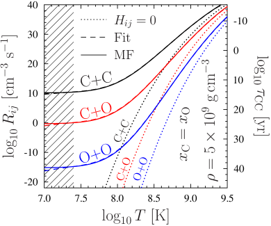
Figure 7: (Color online) Reaction rates in a ¹²C+¹⁶O mixture with $x_{\mathrm{C}}=x_{\mathrm{O}}=0.5$ at $\rho=5\times 10^{9}$ g cm^-3. Solid lines are the mean-field calculations, dashed lines correspond to our fit expression (23), and dotted lines are obtained neglecting the plasma screening. The lines of the same type refer (from top to bottom) to the C+C, C+O, and O+O reactions. The shaded region of $T<2.5\times 10^{7}$ K corresponds to bound Gamow-peak states, $E^{\mathrm{pk}}_{ij}<0$. The right vertical scale shows characteristic carbon burning time $\tau_{\mathrm{CC}}=n_{\mathrm{C}}/R_{\mathrm{CC}}$. See text for details.

Figure 7 shows the temperature dependence of the three (C+C, C+O, and O+O) reaction rates in a ${}^{12}\mathrm{C}$ and ${}^{16}\mathrm{O}$ mixture with equal number density of carbon and oxygen ions at $\rho=5\times 10^{9}$ g cm^-3. The solid lines are our mean-field calculations (marked as MF), the dashed lines are given by the fit expression (23) (marked as Fit), and the dotted lines are calculated neglecting the plasma screening ($H_{ij}(r)=0$). Lines of the same type refer (from top to bottom) to the C+C, C+O, and O+O reactions, respectively. The right vertical scale gives typical carbon burning time $\tau_{\mathrm{CC}}=n_{\mathrm{C}}/R_{\mathrm{CC}}$. The shaded region ($T<2.5\times 10^{7}$ K) corresponds to bound Gamow-peak states (see Fig. 6 and corresponding discussion in the text). This region is similar for all three reactions because of approximately the same charges of reacting ions. For such low temperatures the mean field model with isotropic potential is quantitatively invalid but qualitatively correct; the reaction rates become temperature independent, which is the main property of pycnonuclear burning. The pycnonuclear burning rates are rather uncertain YGABW06 ; typical rates reported in the literature are one order of magnitude smaller than those extracted from our mean field calculations at $T\to 0$. The difference may result from the fact that we use spherically symmetric mean-field potential (rather than more realistic anisotropic potential). In reality, ions can be localized in deeper potential wells near their lattice sites.

The fit and mean-field results, which are mostly indistinguishable in the figure, can strongly differ in the shaded region, especially for the O+O reaction. We do not expect that it is a significant disadvantage of our fit expression (because the mean field approach becomes invalid at such conditions), but we would like to mention this feature. Note, that for the O+O reaction in Fig. 7 the temperature $T=2.5\times 10^{7}$ K corresponds to $\Gamma_{\mathrm{OO}}\approx 400$ and the total enhancement factor is $\sim 10^{110}$.

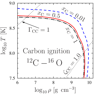
Figure 8: (Color online) Carbon ignition curve in ¹²C+¹⁶O mixtures. Dash-dotted, solid and dashed lines show the mean-field calculations for $x_{\mathrm{C}}=1$, $0.5$, and $0.01$, respectively. We also plot two thin dotted lines of constant $\Gamma_{\mathrm{CC}}=1$ and $\zeta_{\mathrm{CC}}=1$ to demonstrate typical values of dimensionless parameters. See text for details.

Figure 8 presents carbon ignition curves, which are most important for modeling nuclear explosions of massive white dwarfs (supernova Ia events) and carbon explosions in accreting neutron stars (superbursts). For white dwarfs it is determined as a line in the $T-\rho$ plane, where the nuclear energy generation rate equals the local neutrino energy losses (which cool the matter). For higher $T$ and $\rho$ (above the curve), the nuclear energy generation exceeds the neutrino losses and carbon ignites. The curves are plotted for ¹²C+¹⁶O mixtures. The main energy is generated in the C+C reaction even for $x_{\mathrm{C}}=0.01$ because the C+O and O+O reactions are stronger suppressed by the Coulomb barrier (see Fig. 7 to compare the reaction rates). In our mean-field model, which employs the linear mixing, the admixture of oxygen affects the C+C burning only by reducing the number density of carbon nuclei [not through the contact probability $g_{\mathrm{CC}}(0)$; see Eq. (34)], so that the C+C reaction rate is $\propto x_{\mathrm{C}}^{2}$. The neutrino energy losses are mainly produced by plasmon decay and electron-nucleus bremsstrahlung processes. The neutrino emissivity owing to plasmon decay is calculated using the results of Ref. Plasmon (with the online table http://www.ioffe.ru/astro/NSG/plasmon/table.dat). The neutrino bremsstrahlung emissivity is calculated using the formalism of Kaminker et al. kaminkeretal99 , which takes into account electron band structure effects in crystalline matter. For an CO mixture, this neutrino emissivity is determined using the linear mixture rule.

Two thin dotted lines in Fig. 8 correspond to constant $\Gamma_{\mathrm{CC}}=1$ and $\zeta_{\mathrm{CC}}=1$. Dash-dotted, solid and dashed lines are the mean-field calculations for $x_{\mathrm{C}}=1$ (pure carbon matter), $0.5$, and $0.01$, respectively. For a fixed $\rho$, the higher $x_{\mathrm{C}}$ the higher the number density of carbon ions and the higher the reaction rate. This intensifies carbon burning, and the carbon ignites at lower temperature. For high densities, the carbon ignition curve bends and the carbon can ignite at very low temperatures. This is caused by weakening the temperature dependence of the reaction rate (see Fig. 7) and by a strong suppression of neutrino emission with decreasing temperature.

VII Conclusions

We have analyzed the plasma screening enhancement of nuclear reaction rates in binary ionic mixtures. We have used a simple model for the enhancement factor based on the radial WKB tunneling of the reacting nuclei in their Coulomb potential superimposed with the static mean-field potential created by neighboring plasma ions. We have done accurate Monte Carlo calculations of the mean-field plasma potential for a two-component strongly coupled plasma of ions and proposed a simple and accurate analytic fit to the plasma potential (Sec. III). We have calculated the plasma enhancement factors of nuclear reaction rates in the mean-field WKB approximation and have obtained their accurate fit (Sec. IV). We have analyzed the effect of the plasma screening on astrophysical $S$-factors and Gamow-peak energies (Sec. V). To illustrate the results, we analyzed nuclear burning in ¹²C+¹⁶O mixtures (Sec. VI).

We demonstrate that the mean-field WKB method gives qualitatively correct (temperature independent) reaction rates even in the zero-temperature pycnonuclear burning regime. In this regime the dynamics of the reacting ions is determined by zero-point vibrations; they fuse along selected (anisotropic) close-approach trajectories svh69 ; the mean-field radial WKB method was initially expected to be absolutely inadequate. Let us mention in passing that the problem of pycnonuclear burning has not been accurately solved even for OCP plasma (e.g., see OCP_react ), and the uncertainties of the solution increase in multicomponent mixtures (see YGABW06 , and references therein).

Other uncertainties in our knowledge of the reaction rates come from nuclear physics. As a rule, the astrophysical $S$-factors cannot be experimentally measured for such low energies as Gamow peak energies in stellar matter. For example, the lowest experimental point for the ¹²C+¹²C reaction is $\sim 2.1$ MeV, whereas typical Gamow peak energies ${E^{\mathrm{pk}}_{ij}}^{\prime}$ are $\sim 1$ MeV. Therefore, one needs to extrapolate experimental results to lowest energies. Throughout the paper we assumed a smooth energy dependence of astrophysical $S$-factors, that is supported by calculations in the frame of the barrier penetration model (e.g., Ref. Gasetal07 ). However, some models (e.g., Perez_etal06 ), predict resonances at low energy, which can significantly change the reaction rates and ignition curve Cooper_etal09 . We do not discuss such effects in the present paper. New experimental and theoretical studies of astrophysical $S$-factors are needed to solve this problem.

Appendix A Correction of the enhancement factors for weak nonideality

Figure 9: (Color online) The enhancement coefficients $h_{ij}/\Gamma_{\mathrm{e}}^{3/2}$ (at small $\zeta_{ij}$) as a function of $\Gamma_{\mathrm{e}}$ for binary mixtures with $Z_{2}/Z_{1}=2$ and $x_{2}=0.05$ (left), $0.5$ (center) and $0.95$ (right). Thin dotted horizontal lines correspond to Debye-Hückel enhancement (36). Thin solid, dash and long-dash lines are $h_{11}^{\mathrm{lin}}$, $h_{12}^{\mathrm{lin}}$, and $h_{22}^{\mathrm{lin}}$, respectively. Thick lines demonstrate the enhancement factors, calculated using our interpolation expression (39).

Our fit expression (23) does not reproduce the well-known Debye-Hückel enhancement factor for weak Coulomb coupling ($\Gamma_{ij}\ll 1$),

$$h^{\mathrm{DH}}_{ij}=3^{1/2}Z_{i}\,Z_{j}\left<Z^{2}\right>^{1/2}\Gamma_{e}^{3/2}/\left<Z\right>^{1/2}.$$ (36)

Let us remind that $h_{ij}$ is related to the reaction rates by Eq. (18). To correct our approximation in the weak-coupling limit we note, that a formal use of the linear mixing rule [employed in Eq. (23)] at low $\Gamma_{ij}\ll 1$ gives

$$h^{\mathrm{lin}}_{ij}=3^{-1/2}\,\left[\left(Z_{i}+Z_{j}\right)^{5/2}-Z_{i}^{5/2}-Z_{j}^{5/2}\right]\Gamma_{\mathrm{e}}^{3/2}.$$ (37)

Therefore, our fit (23) gives the correct power low ($\propto\Gamma_{\mathrm{e}}^{3/2}$), but an inexact prefactor (for $0.1\leq Z_{1}/Z_{2}\leq 10$ and all $x_{1}$ the relative error does not exceed 40%). We suggest to introduce a correction factor

$$C_{ij}=\frac{h^{\mathrm{DH}}_{ij}}{h^{\mathrm{lin}}_{ij}}=3Z_{i}\,Z_{j}\frac{\left<Z^{2}\right>^{1/2}}{\left<Z\right>^{1/2}}\,\frac{1}{\left(Z_{i}+Z_{j}\right)^{5/2}-Z_{i}^{5/2}-Z_{j}^{5/2}},$$ (38)

and finally write the enhancement factor as

$$h_{ij}=\frac{C_{ij}+\Gamma_{ij}^{2}}{1+\Gamma_{ij}^{2}}\left[f_{0}\left(\frac{\Gamma_{i}}{\tau_{ij}}\right)+f_{0}\left(\frac{\Gamma_{j}}{\tau_{ij}}\right)-f_{0}\left(\frac{\Gamma_{ij}^{\mathrm{comp}}}{\tau_{ij}}\right)\right],$$ (39)

where $\tau_{ij}$ is given by (25). As a result, Eq. (39) reproduces the correct Debye-Hückel asymptote of the enhancement factor in the weak coupling limit ($\Gamma_{ij}\ll 1$) and it reproduces also our results at $\Gamma\gtrsim 1$.

Our interpolation expression is certainly a simplification, but it is expected to be qualitatively correct. In Fig. 9 we show the enhancement factors $h_{ij}$, normalized with respect to $\Gamma_{\mathrm{e}}^{3/2}$, as a function of $\Gamma_{\mathrm{e}}$. We take a BIM with $Z_{2}/Z_{2}$ and $x_{2}=0.05$, $0.5$ and $0.95$ as an example. The thin dotted lines correspond to the Debye-Hückel asymptote at $\Gamma\ll 1$. The thin solid, dash and long-dash lines are the linear mixing asymptotes ($h_{11}^{\mathrm{lin}}$, $h_{12}^{\mathrm{lin}}$, and $h_{22}^{\mathrm{lin}}$, respectively), which are valid in the limit of strong Coulomb coupling, $\Gamma\gg 1$. The thick lines show the enhancement factors, calculated using our interpolation expression (39). One can see that the asymptotes fix the enhancement factors quite well and our interpolation looks reasonable.

Of course, an accurate description of the enhancement factors at moderate Coulomb coupling is desirable but the exact solution may be complicated. Fortunately, in all cases of physical interest the reactions in this regime occur at $\zeta_{ij}\ll 1$, so that we can calculate the enhancement factors as a difference of free energies before and after a reaction event. Recent calculations of Potekhin et al. Potekhin_Mixt of the free energy of binary and triple mixtures at intermediate Coulomb coupling seem to be most important in this respect. However, they are not very convenient for practical purpose because the enhancement factors depend on derivatives of the free energy with respect to numbers of particles. These derivatives should be calculated at small concentrations of compound nuclei, and the accuracy of numerical differentiation deserves a special study.

References

- (1) D. D. Clayton, Principles of Stellar Evolution and Nucleosynthesis (University of Chicago Press, Chicago, 1983).
- (2) P. Höflich, Nucl. Phys. A 777, 579 (2006).
- (3) T. Strohmayer and L. Bildsten, in Compact Stellar X-Ray Sources, edited by W. H. G. Lewin, M. Van der Klis (Cambridge University Press, Cambridge, 2006), p. 113.
- (4) A. Cumming, J. Macbeth, J. J. M. in ’t Zand, and D. Page, Astrophys. J. 646, 429 (2006).
- (5) S. Gupta, E. F. Brown, H. Schatz, P. Moeller, and K.-L. Kratz, Astrophys. J. 662, 1188 (2007)
- (6) D. G. Yakovlev, K. P. Levenfish, Contrib. Plasma Phys. 43, 390 (2003).
- (7) D. G. Yakovlev, K. P. Levenfish, and P. Haensel, Astron. Astrophys. 407, 265 (2003).
- (8) D. G. Yakovlev, K. P. Levenfish, A. Y. Potekhin, O. Y. Gnedin, and G. Chabrier, Astron. Astrophys. 417, 169 (2004).
- (9) D. G. Yakovlev, K. P. Levenfish, O. Y. Gnedin, Eur. Phys. J. A 25, 669-672 (2005).
- (10) D. Page, U. Geppert, and F. Weber, Nucl. Phys. A777, 497 (2006).
- (11) K. P. Levenfish and P. Haensel, Astrophys. Space Sci. 308, 457 (2007).
- (12) P. S. Shternin, D. G. Yakovlev, P. Haensel, and A. Y. Potekhin, Mon. Not. R. Astron. Soc. 382, L43 (2007).
- (13) D. G. Yakovlev, L. Gasques, M. Wiescher, Mon. Not. R. Astron. Soc. 371, 1322 (2006).
- (14) E. E. Salpeter and H. M. Van Horn, Astrophys. J. 155, 183 (1969).
- (15) L. R. Gasques, A. V. Afanasjev, E. F. Aguilera, M. Beard, L. C. Chamon, P. Ring, M. Wiescher, and D. G. Yakovlev, Phys. Rev. C 72, 025806 (2005).
- (16) D. G. Yakovlev, L. R. Gasques, A. V. Afanasjev, M. Beard, and M. Wiescher, Phys. Rev. C 74, 035803 (2006).
- (17) A. I. Chugunov, H.E. DeWitt, D.G. Yakovlev, Phys. Rev. D 76, 025028 (2007).
- (18) J. W. Negele, D. Vautherin, Nucl. Phys. A 207, 298 (1973).
- (19) H. E. DeWitt, W. Slattery, D. Baiko, andr D. Yakovlev, Contrib. Plasma Phys. 41, 251 (2001).
- (20) S. Ichimaru, Rev. Mod. Phys. 65, 255 (1993).
- (21) H. M. Van Horn and E. E. Salpeter, Phys. Rev. 157, 751 (1967).
- (22) S. Schramm and S. E. Koonin, Astrophys. J. 365, 296 (1990); 377, 343(E) (1991).
- (23) N. Itoh, F. Kuwashima, and H. Munakata, Astrophys. J. 362, 620 (1990).
- (24) S. Ogata, Astrophys. J. 481, 883 (1997).
- (25) E. L. Pollock and B. Militzer, Phys. Rev. Lett. 92, 021101 (2004).
- (26) B. Militzer, E. L. Pollock, Phys. Rev. B 71, 134303 (2005).
- (27) A. Alastuey and B. Jancovici, Astrophys. J. 226, 1034 (1978).
- (28) B. Widom, J. Chem. Phys. 39, 2808 (1963).
- (29) B. Jancovici J. Stat. Phys. 17, 357 (1977).
- (30) S. Ogata, H. Iyetomi, and S. Ichimaru, Astrophys. J. 372, 259 (1991).
- (31) H. DeWitt and W. Slattery, Contrib. Plasma Phys. 39, 97 (1999).
- (32) Y. Rosenfeld, Phys. Rev. E 53, 2000 (1996).
- (33) H. DeWitt, W. Slattery and G. Chabrier, Physica B 228, 21 (1996).
- (34) H. DeWitt and W. Slattery, Contrib. Plasma Phys. 43, 279 (2003).
- (35) A. Y. Potekhin, G. Chabrier, F. J. Rogers, Phys. Rev. E 79, 016411 (2009).
- (36) J.-M. Caillol and D. Gilles, J. Phys. A 36, 6243 (2003).
- (37) S. Ogata, S. Ichimaru, and H. M. Van Horn, Astrophys. J. 417, 265 (1993).
- (38) A. Y. Potekhin and G. Chabrier, Phys. Rev. E 62, 8554 (2000).
- (39) E. E. Salpeter, Aust . J. Phys. 7, 373 (1954).
- (40) H. E. DeWitt, H. C. Graboske, and M. S. Cooper, Astrophys. J. 181, 439 (1973).
- (41) D. G. Yakovlev and D. A. Shalybkov, Soviet Sci. Rev. Sec. E 7, 313 (1989).
- (42) L. R. Gasques, A. V. Afanasjev, M. Beard, J. Lubian, T. Neff, M. Wiescher, and D. G. Yakovlev, Phys. Rev. C 76, 045802 (2007).
- (43) N. Itoh, N. Tomizawa, S. Wanajo, and S. Nozawa, Astrophys. J. 586, 1436 (2003).
- (44) C. L. Jiang, K. E. Rehm, B. B. Back, and R. V. F. Janssens, Phys. Rev. C 75 015803 (2007).
- (45) E. M. Kantor, M. E. Gusakov, MNRAS 381, 1702-1710 (2007).
- (46) A. D. Kaminker, C. J. Pethick, A. Y. Potekhin, V. Thorsson, and D. G. Yakovlev, Astron. Astrophys. 343, 1009 (1999).
- (47) R. Perez-Torres, T.L. Belyaeva, E. F. Aguilera, Physics of Atomic Nuclei 69, 1372 (2006).
- (48) R. L. Cooper, A. W. Steiner, and E. F. Brown, arXiv:0903.3994.