Abstract

We study general conditions for the gravitino to be the lightest supersymmetric particle (LSP) in models with gravity mediated supersymmetry breaking. We find that the decisive quantities are the Kähler potential $K$ and the gauge kinetic function $f$. In constrained MSSM (CMSSM) type models, the gravitino LSP occurs if the gaugino mass at the GUT scale is greater than approximately 2.5 gravitino masses. This translates into $\sqrt{K^{\prime\prime}}/f^{\prime}<0.2$, where the derivatives are taken with respect to the dominant SUSY breaking field. This requirement can easily be satisfied in string-motivated setups.

1 Introduction

It is an exciting possibility that dark matter has a supersymmetric origin. Various species can have the properties of dark matter depending on the supersymmetry breaking mechanism and further particulars of the model, with the neutralino and gravitino being the most prominent candidates.

In classes of models like anomaly [1] and mirage [2] mediation, the gravitino is heavier than the other sparticles and thus cannot constitute dark matter. On the other hand, in gauge [3] and gaugino [4] mediation, the gravitino is light and represents a good candidate for dark matter [3],[5]. In gravity mediation [6], the situation is more model-dependent and both relatively heavy and light gravitinos are possible. In this work, we study the circumstances under which the gravitino is the LSP in gravity mediation. If we further require R- or matter parity [7], which can descend from string theory [8], the gravitino is stable and can constitute dark matter. Phenomenology of the gravitino LSP has been an active research subject [9]–[14], while in this paper we focus on its supergravity side and identify relevant constraints on fundamental supergravity quantities.

2 Supergravity preliminaries

Let us review relevant features of the supergravity formalism, following [15] (and the original work [16]). The supergravity scalar potential is given (in Planck units) by

$$V=\bar{F}^{\bar{i}}F^{j}K_{\bar{i}j}-3~{}{\rm e}^{G}~{}.$$ (1)

Here the subscript $l$ ($\bar{l}$) denotes differentiation with respect to the $l$-th ($l$-th complex conjugate) scalar field. $G$ is a function of the Kähler potential $K$ and the superpotential $W$, $G=K+\ln(|W|^{2})$, and the SUSY breaking $F$-terms are $F^{i}={\rm e}^{G/2}K^{i\bar{j}}G_{\bar{j}}$ with $K^{i\bar{j}}$ being the inverse of $K_{\bar{i}j}$. The gravitino mass is given by

$$m_{3/2}={\rm e}^{G/2}\;.$$ (2)

Another quantity we need is the Kähler metric $\tilde{K}_{\alpha}$ for the observable fields $\phi^{\alpha}$. It is found by expanding the Kähler potential around $\phi^{\alpha}=0$ :

$$K=K\Big{|}_{\phi_{\alpha}=0}+\tilde{K}_{\alpha}\phi^{*\bar{\alpha}}\phi^{\alpha}+...$$ (3)

Then the soft SUSY breaking terms are given by [15]

$$M_{a} = {1\over 2}({\rm Re}f_{a})^{-1}F^{m}\partial_{m}f_{a}\;,$$ (4)

$$m_{\alpha}^{2} = m^{2}_{3/2}-\bar{F}^{\bar{m}}F^{n}\partial_{\bar{m}}\partial_{n}\ln\tilde{K}_{\alpha}\;,$$

$$A_{\alpha\beta\gamma} = F^{m}\left[K_{m}+\partial_{m}\ln Y_{\alpha\beta\gamma}-\partial_{m}\ln(\tilde{K}_{\alpha}\tilde{K}_{\beta}\tilde{K}_{\gamma})\right]\;,$$

where $f_{a}$ are the gauge kinetic functions,

$${\rm Re}f_{a}={1\over g^{2}_{a}}~{},$$ (5)

$\partial_{m}\equiv\partial/\partial\phi^{m}$, and $Y_{\alpha\beta\gamma}$ are the superpotential Yukawa couplings.

Vanishing of the vacuum energy requires

$$\bar{F}^{\bar{i}}F^{j}K_{\bar{i}j}=3\,m_{3/2}^{2}$$ (6)

at the minimum of the scalar potential. Thus, the magnitude of the $F$-terms depends on the Kähler metric of the SUSY breaking fields $K_{\bar{i}j}$. The $F$-terms and, consequently, the soft masses can be much larger than the gravitino mass provided the Kähler metric is sufficiently small.

3 Gravitino LSP

Let us consider the case of a single dominant SUSY breaking field $C$. Omitting for simplicity complex phases, we have

$$F=\sqrt{3\over K^{\prime\prime}}~{}m_{3/2}\;,$$ (7)

where $K^{\prime\prime}\equiv K_{\bar{C}C}$. Let us further assume universal gauge kinetic functions and Kähler metrics for the matter fields. Then the soft terms simplify to

$$m_{1/2} = \sqrt{3\over 4K^{\prime\prime}}~{}g^{2}f^{\prime}~{}m_{3/2}~{},$$

$$m_{0}^{2} = \biggl{[}1-3{\tilde{K}^{\prime\prime}\tilde{K}-{\tilde{K}}^{{}^{\prime}2}\over K^{\prime\prime}\tilde{K}^{2}}\biggr{]}~{}m_{3/2}^{2}~{},$$

$$A_{0} = \sqrt{3\over K^{\prime\prime}}~{}\biggl{[}K^{\prime}-3{\tilde{K}^{\prime}\over\tilde{K}}\biggr{]}~{}m_{3/2}~{},$$ (8)

where a prime denotes differentiation with respect to $C$ and a double prime differentiation with respect to $C$ and $\bar{C}$. We have assumed that the Yukawa couplings are independent of $C$, which allows us to avoid strong constraints from electric dipole moments [17].

This case corresponds to the CMSSM. We see that the scalar and gaugino masses can be made arbitrarily large by decreasing $K^{\prime\prime}$. This requires a non-negligible $f^{\prime}$ and $\tilde{K}^{\prime\prime}\tilde{K}-{\tilde{K}}^{{}^{\prime}2}\leq 0$. If this quantity vanishes at the GUT scale, large scalar masses are induced by the renormalization group evolution down to the electroweak (EW) scale. Since the gravitino mass does not run, we have

$$M_{i}\;,\;m_{\alpha}\,>\,m_{3/2}$$ (9)

and the gravitino is the LSP. The $A$-terms usually do not play any significant role unless they are much larger than the other soft parameters.

Let us quantify this effect. In the CMSSM, the lightest superparticle is either a neutralino (mostly bino) or a stau. Unless $\tan\beta$ is large, their masses can be approximated by [18],[19]

$$m_{\chi} \simeq 0.4\,m_{1/2}\;,$$

$$m^{2}_{\tilde{\tau}} \simeq m_{0}^{2}+0.15\,m_{1/2}^{2}\;,$$ (10)

where we have neglected the EW contributions. For moderate $m_{0}$, the lightest neutralino is lighter than the staus. Then the gravitino is the LSP for

$$m_{1/2}>2.5\,m_{3/2}\;.$$ (11)

For small $m_{0}$, the stau is lighter than the neutralino, so that a larger $m_{1/2}$ is required for a gravitino LSP. However, Eq. (10) shows that the change in the lower bound will be rather small, so that Eq. (11) is still a good approximation.

Thus, the key parameter is the gaugino mass $m_{1/2}$ and as long as the scalar masses squared are non-negative, we obtain the gravitino LSP for

$${\sqrt{K^{\prime\prime}}\over f^{\prime}}<0.2\;,$$ (12)

where we have used $g^{2}(M_{\rm GUT})\simeq 1/2$. This bound does not involve the superpotential nor the Kähler metric for the observable fields and is therefore largely model-independent.

In Figs. 1 and 2 we illustrate these results with a numerical analysis in the CMSSM. We have used SOFTSUSY [23] to determine the low-energy superpartner spectrum. The figures display parameter space regions with the gravitino, neutralino and stau LSP. We have chosen $m_{3/2}=400$ GeV to fix the overall mass scale for definiteness, while the qualitative features of the plots are independent of this.

At large $\tan\beta$, Eq. (10) receives corrections mainly from the $\tau$ Yukawa coupling so that the $\tilde{\tau}$ becomes the LSP at small $m_{0}$. This is displayed in the right panel of Fig. 1. Also, large $A$-terms further decrease the stau mass and can lead to tachyons, so that the $\tilde{\tau}$ LSP and the excluded regions are enlarged, cf. Fig. 2.

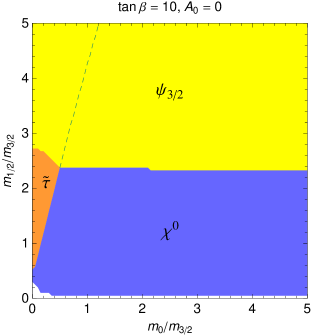
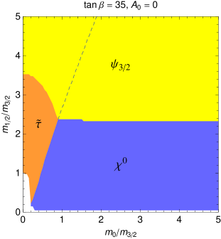
Figure 1: Regions with different LSPs in the CMSSM. In the region to the left of the dashed line, the stau is the next-to-LSP (NLSP), while to the right the lightest neutralino is the NLSP. The white area at the bottom of each plot is excluded because of tachyons or no EW symmetry breaking. For definiteness, we have fixed $m_{3/2}=400$ GeV and $\mu>0$.

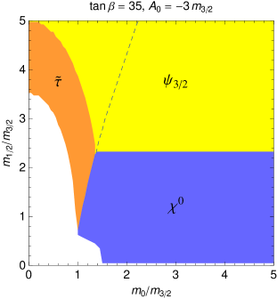
Figure 2: Same as Fig. 1, but with a large $A$-term.

Let us note that our parameter space is subject to further (model-dependent) phenomenological constraints. These depend on the overall mass scale, assumptions on the cosmological history, whether R-symmetry is exact or approximate and whether the gravitino constitutes all or just part of the observed dark matter. For instance, as the LEP bound on the Higgs mass requires $m_{1/2}\gtrsim 400$ GeV, Eq. (8) implies $m_{3/2}\gtrsim 10^{2}$ GeV for $\sqrt{K^{\prime\prime}}=\mathcal{O}(10^{-1})$ and $f^{\prime}=\mathcal{O}(1)$. For detailed studies, we refer an interested reader to Refs. [9]–[14].

From Eq. (12), we see that $K^{\prime\prime}$ is not required to be very small. In fact, it is of the order of magnitude of typical $K^{\prime\prime}$ expected in string theory. The usual moduli/dilaton Kähler potential is $K=-a\ln(C+\bar{C})$ with $a={\cal O}(1)$ so that

$$\sqrt{K^{\prime\prime}}={\sqrt{a}\over C+\bar{C}}\;.$$ (13)

Just to have an idea of the numerics, take $C$ to be the dilaton of the heterotic string. Then $a=1$, $f=C$ and $C=2$ at the minimum of the potential, as required by the observed values of the gauge couplings. We get ${\sqrt{K^{\prime\prime}}\over f^{\prime}}=0.25$, which falls just short of the bound (12). One should keep in mind, however, that the dilaton-dominated SUSY breaking is not possible with the above Kähler potential and in realistic cases one has to include either non-perturbative corrections to the Kähler potential [24],[25] or additional fields. In the former case, one typically has $K^{\prime\prime}\ll 1$ at the minimum of the potential [26],[27], although the zero vacuum energy is not enforced.

When $C$ is the modulus associated with the radius of the compact dimensions, one can trust the supergravity approximation for $C\gg 1$ in which case $\sqrt{K^{\prime\prime}}$ can be arbitrarily small. In realistic cases, however, one has to include more than one field to have the correct gauge coupling, e.g. $f=C_{1}+C_{2}$. Otherwise, the gauge coupling becomes too small.

One can also entertain the possibility that $C$ is a hidden matter-like field with the Kähler potential $K={\rm const}+\kappa\bar{C}C$, which dominates SUSY breaking [28]. In this case, $\kappa$ can be very small due to large moduli, $\kappa=1/(T+\bar{T})^{n}$. However, the gauge kinetic function is then given predominantly by some other field, e.g. the dilaton, so that $f^{\prime}\ll 1$. Consequently, $\sqrt{K^{\prime\prime}}/f^{\prime}$ can be sufficiently small for the gravitino to be the LSP, yet $\sqrt{K^{\prime\prime}}/f^{\prime}\ll 1$ would require careful engineering.

The above formulae can be generalized to the case of multiple SUSY breaking fields in a straightforward manner.

3.1 Semi-realistic example

Let us illustrate with an example how the gravitino LSP can arise in string-motivated setups. Consider two modulus-type fields $C_{1}$ and $C_{2}$ with

$$K^{\rm hid}=-a\ln(C_{1}+\bar{C}_{1})-b\ln(C_{2}+\bar{C}_{2})~{},$$

$$\tilde{K}=(C_{1}+\bar{C}_{1})^{n}~{},$$

$$f=C_{1}-C_{2}\;,$$ (14)

and $a,b>0$. Here $n$ is the matter “modular weight”, which can be negative, positive or zero [29]. For $a+b>3$, locally stable vacua with zero (or small) vacuum energy are possible [30]. For instance, this is the case when $C_{1,2}$ are the overall modulus and the dilaton. Finally, one can choose an appropriate superpotential such that the fields stabilize at

$$(C_{1}-C_{2})|_{\rm min}\simeq 2\;,$$ (15)

in order to have the correct gauge couplings at the GUT scale. “Mixed” gauge kinetic functions of this type appear in string models with fluxes [31],[32].

Requiring zero vacuum energy at the minimum of the scalar potential and neglecting complex phases, we can parametrize supersymmetry breaking by the Goldstino angle $\theta$:

$$F_{1}=\sqrt{3\over K^{\rm hid}_{C_{1}\bar{C}_{1}}}~{}m_{3/2}~{}\cos\theta~{}~{},~{}~{}F_{2}=\sqrt{3\over K^{\rm hid}_{C_{2}\bar{C}_{2}}}~{}m_{3/2}~{}\sin\theta~{}~{}.$$ (16)

Then the soft terms read

$$m_{1/2} = \sqrt{3\over 4}~{}g^{2}\Biggl{[}{C_{1}+\bar{C}_{1}\over\sqrt{a}}~{}\cos\theta-{C_{2}+\bar{C}_{2}\over\sqrt{b}}~{}\sin\theta\Biggr{]}~{}m_{3/2}~{},$$

$$m_{0}^{2} = \biggl{[}1+{3n\over a}~{}\cos^{2}\theta\biggr{]}~{}m_{3/2}^{2}~{},$$

$$A_{0} = -\sqrt{3}~{}\biggl{[}\sqrt{a}\left(1+{3n\over a}\right)~{}\cos\theta+\sqrt{b}~{}\sin\theta\biggr{]}~{}m_{3/2}~{}.$$ (17)

For a sufficiently large $C_{1}$ and $C_{2}=C_{1}-2$, the gauginos are heavy so that $|m_{1/2}|>2.5\,m_{3/2}$ and the gravitino is the LSP. Note that the $C_{i}$ dependence cancels out in $m_{0}^{2}$ and $A_{0}$.

Taking as an example $C_{1,2}$ to be the overall modulus and the dilaton, $a=3$ and $b=1$. Then for $\cos\theta\sim 1$, the gravitino LSP imposes the bound $C_{1}>5$. Note that the scalar masses are non-tachyonic at the GUT scale for $n\geq-1$.

Let us finally note that the superpotential does not play a role in this discussion as long as it stabilizes the fields at the desired values with vanishing vacuum energy. This question can be analyzed locally, in terms of $\delta C_{1}\equiv C_{1}-C_{1}|_{\rm min}$ and $\delta C_{2}\equiv C_{2}-C_{2}|_{\rm min}$, along the lines of Ref. [28]. As a result, the superpotential expansion coefficients $x_{a}$, $W=x_{0}+x_{1}~{}\delta C_{1}+x_{2}~{}\delta C_{2}+x_{11}~{}(\delta C_{1})^{2}+x_{12}~{}\delta C_{1}\delta C_{2}+x_{22}~{}(\delta C_{2})^{2}+...$, have to satisfy certain (model-dependent) constraints.

4 Conclusions

We have studied the conditions for the gravitino to be the LSP in models of gravity mediated SUSY breaking. This requirement constrains mainly the gaugino mass parameter at the GUT scale while the other parameters play a minor role, as long as the scalar masses are non-tachyonic. For CMSSM-type models at moderate $\tan\beta$, the resulting constraint on the Kähler potential and the gauge kinetic function is approximately $\sqrt{K^{\prime\prime}}/f^{\prime}<0.2$, where the derivatives are taken with respect to the dominant SUSY breaking field. For large $\tan\beta$ and $A$-terms, the above constraint gets modified at small values of the universal scalar mass $m_{0}$. The results are illustrated in Figs. 1 and 2.

The condition $\sqrt{K^{\prime\prime}}/f^{\prime}<0.2$ can easily be satisfied in string-motivated set-ups and thus the gravitino LSP is a reasonable alternative to the neutralino LSP in gravity mediation. As it is hard to obtain an extremely small value of $K^{\prime\prime}$ without finetuning, the gravitino mass is still expected to be of the same order of magnitude as the other soft masses.

References

- [1] L. Randall and R. Sundrum, Nucl. Phys. B 557, 79 (1999); G. F. Giudice, M. A. Luty, H. Murayama and R. Rattazzi, JHEP 9812, 027 (1998).
- [2] K. Choi, A. Falkowski, H. P. Nilles and M. Olechowski, Nucl. Phys. B 718, 113 (2005); M. Endo, M. Yamaguchi and K. Yoshioka, Phys. Rev. D 72, 015004 (2005); K. Choi, K. S. Jeong and K.-i. Okumura, JHEP 0509, 039 (2005); A. Falkowski, O. Lebedev and Y. Mambrini, JHEP 0511, 034 (2005).
- [3] M. Dine, W. Fischler and M. Srednicki, Nucl. Phys. B 189, 575 (1981); M. Dine and W. Fischler, Phys. Lett. B 110, 227 (1982); M. Dine and A. E. Nelson, Phys. Rev. D 48, 1277 (1993); M. Dine, A. E. Nelson and Y. Shirman, Phys. Rev. D 51, 1362 (1995).
- [4] D. E. Kaplan, G. D. Kribs and M. Schmaltz, Phys. Rev. D 62, 035010 (2000); Z. Chacko, M. A. Luty, A. E. Nelson and E. Ponton, JHEP 0001, 003 (2000);
- [5] W. Buchmüller, K. Hamaguchi and J. Kersten, Phys. Lett. B 632, 366 (2006); W. Buchmüller, L. Covi, J. Kersten and K. Schmidt-Hoberg, JCAP 0611, 007 (2006); J. L. Evans, D. E. Morrissey and J. D. Wells, Phys. Rev. D 75, 055017 (2007).
- [6] H. P. Nilles, Phys. Lett. B 115, 193 (1982).
- [7] S. Dimopoulos, S. Raby and F. Wilczek, Phys. Lett. B 112, 133 (1982).
- [8] O. Lebedev, H. P. Nilles, S. Raby, S. Ramos-Sanchez, M. Ratz, P. K. S. Vaudrevange and A. Wingerter, Phys. Rev. D 77, 046013 (2008).
- [9] T. Moroi, H. Murayama and M. Yamaguchi, Phys. Lett. B 303, 289 (1993); T. Kanzaki, M. Kawasaki, K. Kohri and T. Moroi, Phys. Rev. D 75, 025011 (2007).
- [10] J. R. Ellis, K. A. Olive, Y. Santoso and V. C. Spanos, Phys. Lett. B 588, 7 (2004); J. R. Ellis, K. A. Olive and Y. Santoso, JHEP 0810, 005 (2008).
- [11] W. Buchmüller, K. Hamaguchi, M. Ratz and T. Yanagida, Phys. Lett. B 588, 90 (2004); K. Hamaguchi, S. Shirai and T. T. Yanagida, Phys. Lett. B 663, 86 (2008).
- [12] J. L. Feng, S. Su and F. Takayama, Phys. Rev. D 70, 063514 (2004); Phys. Rev. D 70, 075019 (2004).
- [13] L. Roszkowski, R. Ruiz de Austri and K. Y. Choi, JHEP 0508, 080 (2005); S. Bailly, K. Y. Choi, K. Jedamzik and L. Roszkowski, arXiv:0903.3974 [hep-ph].
- [14] A. Brandenburg, L. Covi, K. Hamaguchi, L. Roszkowski and F. D. Steffen, Phys. Lett. B 617, 99 (2005); F. D. Steffen, JCAP 0609, 001 (2006).
- [15] A. Brignole, L. E. Ibáñez and C. Muñoz, arXiv:hep-ph/9707209.
- [16] S. K. Soni and H. A. Weldon, Phys. Lett. B 126, 215 (1983); V. S. Kaplunovsky and J. Louis, Phys. Lett. B 306, 269 (1993).
- [17] S. Abel, S. Khalil and O. Lebedev, Phys. Rev. Lett. 89, 121601 (2002).
- [18] D. G. Cerdeño, K. Y. Choi, K. Jedamzik, L. Roszkowski and R. Ruiz de Austri, JCAP 0606, 005 (2006).
- [19] S. P. Martin and P. Ramond, Phys. Rev. D 48, 5365 (1993).
- [20] A. Riotto and E. Roulet, Phys. Lett. B 377, 60 (1996); A. Kusenko, P. Langacker and G. Segre, Phys. Rev. D 54, 5824 (1996).
- [21] A. Riotto, E. Roulet and I. Vilja, Phys. Lett. B 390, 73 (1997).
- [22] J. R. Ellis, J. Giedt, O. Lebedev, K. Olive and M. Srednicki, Phys. Rev. D 78, 075006 (2008).
- [23] B. C. Allanach, Comput. Phys. Commun. 143, 305 (2002)
- [24] P. Binetruy, M. K. Gaillard and Y. Y. Wu, Nucl. Phys. B 481, 109 (1996).
- [25] J. A. Casas, Phys. Lett. B 384, 103 (1996).
- [26] T. Barreiro, B. de Carlos and E. J. Copeland, Phys. Rev. D 57, 7354 (1998).
- [27] W. Buchmüller, K. Hamaguchi, O. Lebedev and M. Ratz, Nucl. Phys. B 699, 292 (2004).
- [28] O. Lebedev, H. P. Nilles and M. Ratz, Phys. Lett. B 636, 126 (2006); O. Lebedev, V. Löwen, Y. Mambrini, H. P. Nilles and M. Ratz, JHEP 0702, 063 (2007).
- [29] L. E. Ibáñez and D. Lüst, Nucl. Phys. B 382, 305 (1992).
- [30] M. Gomez-Reino and C. A. Scrucca, JHEP 0605, 015 (2006).
- [31] D. Lüst, P. Mayr, R. Richter and S. Stieberger, Nucl. Phys. B 696, 205 (2004).
- [32] H. Abe, T. Higaki and T. Kobayashi, Phys. Rev. D 73, 046005 (2006).