Unravelling the size distribution of social groups with information theory on complex networks

Abstract

The minimization of Fisher’s information (MFI) approach of Frieden et al. [Phys. Rev. E 60 48 (1999)] is applied to the study of size distributions in social groups on the basis of a recently established analogy between scale invariant systems and classical gases [arXiv:0908.0504]. Going beyond the ideal gas scenario is seen to be tantamount to simulating the interactions taking place in a network’s competitive cluster growth process. We find a scaling rule that allows to classify the final cluster-size distributions using only one parameter that we call the competitiveness. Empirical city-size distributions and electoral results can be thus reproduced and classified according to this competitiveness, which also allows to correctly predict well-established assessments such as the “six-degrees of separation”, which is shown here to be a direct consequence of the maximum number of stable social relationships that one person can maintain, known as Dunbar’s number. Finally, we show that scaled city-size distributions of large countries follow the same universal distribution.

1 Introduction

Regularities reflected in either scaling properties bat1 or power laws city1 ; power ; pareto appear in different scenarios related to social groups. One of the most intriguing is Zipf’s law zipf , a power law with exponent $-2$ for the density distribution function that is observed in describing urban agglomerations ciudad and firm sizes all over the world firms . This fact has received a remarkable degree of attention in the literature. The above mentioned regularities have been detected in other contexts as well, ranging from percolation theory and nuclear multi-fragmentation perco to the abundances of genes in various organisms and tissues furu , the frequency of words in natural languages zipf ; zip , the scientific collaboration networks cites , the total number of cites of physics journals nosotrosZ , the Internet traffic net1 or the Linux packages links linux . More recently, R. N. Costa Filho et al. elec1 found another special regularity in the density distribution function of the number of votes in the Brazilian elections, a power law with exponent $-1$. This law has also been found in Ref. nosotros , using an information-theoretic methodology alp , for both the city-size distribution of the province of Huelva (Spain) and the results of the 2008 Spanish General Elections. These findings allow one to conjecture that this behavior reflects a second class of universality.

What all these disparate systems have in common is the lack of a characteristic size, length or frequency for the observable under scrutiny, which makes them scale-invariant. In Ref. nosotros we have introduced an information-theoretic technique based upon the minimization of Fisher’s information measure alp (abbreviated as MFI) that allows for the formulation of a “thermodynamics” for scale-invariant systems. The methodology establishes an analogy between such systems and physical gases which, in turn, shows that the two special power laws mentioned in the preceding paragraph lead to a set of relationships formally identical to those pertaining to the equilibrium states of a scale invariant non-interacting system, the scale-free ideal gas (SFIG). The difference between the two distributions is thereby attributed to different boundary conditions on the SFIG.

However, there are many social systems that can not be included into any of these two universality classes and exhibit different kinds of behavior nosotros . In order to deal with them, during the last years researchers have worked out different mathematical models and thus addressed urban dynamics ud and electoral results elec1 ; elec2 , developing detailed realistic approaches. Ref. otros is highly recommendable as a primer on urban modelling. However, some aspects of the concomitant problems defy full understanding, since a clear prescription for the classification of the size-distribution of social groups is still missing. To remedy such an understanding-gap is our main purpose here.

The goals and motivation of this work are thus focussed on gaining insight into such size-distributions in the case of systems that can not be described by recourse to the two power laws described above, i.e., by a non-interacting scenario. If an analogy with real gases is worked out when interactions are duly taken into account, a microscopic description is needed in order to obtain the pair correlation function MD . This is achieved using numerical simulations as in molecular dynamics. An similar path will be followed here by recourse to the Fisher-derived analogy of nosotros . Thereby we go beyond the SFIG stage by using a proportional growth process (PGP) so as to model the interaction between the elements of the social network system. We can thus study the PGP effect on the density distribution. This requires to have at hand a way to properly describe scale invariance at the microscopic level nosotros ; exp via a competitive cluster growth process within a complex network.

This work is organized as follows: in Sec. II we describe the application of the MFI approach alp to complex networks in order to obtain the degree distribution and thus describe the competitive cluster growth process (inside the network). This allows one to, in turn, microscopically simulate growth processes in a social group. In Sec. III we study the size distributions obtained using this methodology. We find a scale transformation that allows for systematically classifying the deviations from the SFIG that we encounter in the cluster-size distributions. This classification is effected using just a single parameter, which we call the competitiveness. We also apply this criterion to classify the city-size distributions of the provinces of Spain and some electoral results. Moreover, we show that empirical assessments as the average path length and Dunbar’s number are well reproduced by our approach. Using such a scale transformation we demonstrate that most distributions of city population in large countries exhibit the same shape. Finally, in Sec. IV we draw some conclusions.

2 Theoretical method

City-size distributions and electoral results display a similar scale-free behavior, and both of them have the same constituents: groups of people. Although the resources of these groups or the interests of the individuals composing them may be different in each case, a naive approach is to assume that people are connected to other people, hence giving rise to a network where groups of interest develop. Network theory net1 has been successfully used before for dealing with electoral results and the spread of opinions, which encourages to employ it to develop the microscopic description of the associated systems.

2.1 The scale free ideal network

The basic elements of networks are “nodes” that are connected to other nodes by “edges”. The degree $k$ of each node is defined as the number of connections it possesses. The degree distribution (DD) $F(k)$ and the way the nodes are connected define the statistical properties of the network. Scale-free complex networks display many interesting properties that have been found in techno-sociological systems such as the Internet (World Wide Web bbaa , e-mail networks email and also instant-message-sending networks mess , for example).

In our model, we assume that the network can be described at the macroscopic level as a scale invariant system of $N$ nodes, with the number of connections $k$ the “coordinate” that locates each node in the pertinent configuration space. We also assume that the degree of each node does not depend on the degree of other nodes. In these circumstances we can i) legitimately describe the network as a SFIG in an equilibrium state, a scenario to be denoted as the scale free ideal network (SFIN), and ii) derive the DD via the MFI, which we pass now to recapitulate.

2.1.1 Minimum Fisher Information approach (MFI)

The Fisher information measure $I$ for a system of $N$ elements, described by the coordinate $k$ and the physical parameters $\theta$ has the form libro

$$I(F)=c_{k}\int dkF(k|\theta)\left|\frac{\partial\ln F(k|\theta)}{\partial\theta}\right|^{2},$$ (1)

where $F(k|\theta)$ is the density distribution in configuration space and the constant $c_{k}$ accounts for proper dimensionality. According to MFI tenets alp , the equilibrium state of the system minimizes $I$ subject to prior conditions, such as the normalization of $F$, namely $\langle 1\rangle=1$. The MFI is then cast as a variation problem of the form alp

$$\delta\left\{I(F)-\mu\langle 1\rangle\right\}=0,$$ (2)

where $\mu$ is the normalization-associated Lagrange multiplier.

2.1.2 Application of the MFI to a scale-free network

In the case of the derivation of the DD of our complex network, we define a minimum degree of unity and a maximum degree value of $k_{M}$. With the change of variable $u=\ln k$, the scale transformation $k^{\prime}=k/\theta_{k}$ transforms $u$ into $u^{\prime}=u-\Theta_{k}$, where $\Theta_{k}=\ln\theta_{k}$. The distribution of physical elements is then described by the mono-parametric translation families $F(k|\theta)=f(u|\Theta_{k})=f(u^{\prime})$. Taking into account the fact that the Jacobian of the transformation is $dk=e^{u}du$, the information measure $I$ can be obtained in the continuous limit as

$$I=c_{u}\int_{0}^{\ln k_{M}}\!\!\!du~{}e^{u}f(u)\left|\frac{\partial\ln f(u)}{\partial u}\right|^{2},$$ (3)

and, with the normalization constraint

$$\int_{0}^{\ln k_{M}}\!\!\!du~{}e^{u}f(u)=1,$$ (4)

the variation problem reads now

$$\delta\left\{c_{u}\int_{0}^{\ln k_{M}}\!\!\!du~{}e^{u}f\left|\frac{\partial\ln f}{\partial u}\right|^{2}+\mu\int_{0}^{\ln k_{M}}\!\!\!du~{}e^{u}f\right\}=0.$$ (5)

Introducing $f(u)=e^{-u}\Psi^{2}(u)$, and varying with respect to $\Psi$ leads to the Schrödinger-like equation alp

$$\left[-4\frac{\partial^{2}}{\partial u^{2}}+1+\mu^{\prime}\right]\Psi(u)=0,$$ (6)

where $\mu^{\prime}=\mu/c_{u}$. The general solution to this equation is $\Psi(u)=e^{-\alpha u/2}$ with $\alpha=\sqrt{1+\mu^{\prime}}$. Equilibrium corresponds to the ground state solution $\alpha=0$ alp , which yields the same density distribution as that of the SFIG in the thermodynamic limit

$$F(k)dk=\frac{1}{\ln k_{M}}\frac{dk}{k}.$$ (7)

Once we know, for a given total number of nodes $N$, the associated DD of the SFIN, we proceed by assigning a number of potential edges $k$ to each node, with $k$ randomly obtained from $F(k)$. Accordingly, the $N$ nodes are randomly connected among themselves by their assigned edges, with two restrictions: a node cannot be connected to itself nor twice to the same node. The ensuing process ends when no more connections can be established. We will show later that the values of $N$ and $k_{M}$ can be arbitrarily chosen in order to classify the empirical distributions.

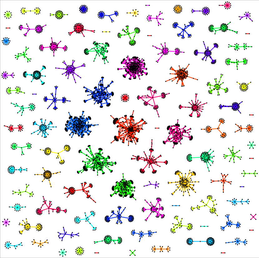
Figure 1: (Color online) Final result of a competitive process of $n_{c}=100$ clusters with an initial size of $n_{i}=1$ nodes in a network of $N=5\,000$ nodes. All the clusters belong to the same network and are connected among themselves. For clarity’s sake, however, they have been plotted independently. A large variety of cluster sizes ensues.

2.2 The competitive cluster growth process

Once we have built a SFIN with $N$ nodes and maximum degree $k_{M}$, we apply a competitive cluster growth process to it, as discussed in bran . This technique falls into the category of PGP or discrete multiplicative processes, which are known to correctly describe scale-invariant behavior exp . For starters, we fix the values of the minimum cluster size $n_{i}$ and the total number of clusters $n_{c}$ that will grow in the network. Next, $n_{c}\times n_{i}$ nodes of the network are randomly selected as cluster “seeds”. In the first iteration the first neighbors of the seeds are incorporated to the cluster in random order, unless they are seeds of other clusters. At subsequent iterations, the first neighbors of the nodes added at the precedent step are, in turn, randomly added to the cluster, unless they already belong to a different cluster. The process ends when all the nodes belong to some cluster. We display in Fig. 1 the final result of a competitive growth process for $n_{c}=100$ clusters with an initial size of $n_{i}=1$ node in a network of $5\,000$ nodes.

The procedure may include a probability $t$ for a node changing to another cluster if any of its neighbors belongs to this cluster (micro-dynamics). However, M. Batty found that even if the rank of the cities rapidly evolves in time due to micro-dynamics, the city-size distribution evolves only slowly clock : the system evolves quasi-statically at the macroscopic level. We then consider that the system exhibits an adiabatic evolution, implying that our distributions can be well represented by stationary configurations ($t=0$). Although not at this stage, we expect to study micro-dynamics in the future.

3 Present results

3.1 Study and classification of cluster-size distributions

3.1.1 Regime of low-density of clusters: recovering the SFIG

We have studied the size distribution of SFIN-clusters with $N$ and $k_{M}$ ranging from $N=5\,000$ to $500\,000$ and $k_{M}=50$ to $500$ —finite-size effects may be relevant for smaller values of $N$ and $k_{M}$. When the density of seeds, defined as $\rho_{s}=n_{c}n_{i}/N$, is much lower than unity, the probability density distribution of sizes $p(x)$ mostly follows that of the SFIG at equilibrium, which is in the continuous limit

$$p(x)dx=\begin{cases}\dfrac{1}{\Omega}\dfrac{dx}{x}&\text{if }x_{1}\leq x\leq x_{M}\\ 0&\text{otherwise}\end{cases},$$ (8)

where $\Omega=\ln(x_{M}/x_{1})$ is the “volume” in the concomitant size-configuration space. The maximum $x_{M}$ and minimum $x_{1}$ sizes generally depend on $n_{i}$, $n_{c}$, and $N$. Since finite-size effects make it difficult to estimate $x_{1}$ and $x_{M}$, we have found it useful to evaluate the volume as $\Omega=2\ln(x_{3/4}/x_{1/4})$, where $x_{1/4}$ and $x_{3/4}$ indicate the first and third quartiles of the distribution.

It is convenient for a scale-invariant system to introduce a new variable $x^{\prime}=x/\theta$ without changing the physics, with $\theta$ a parameter to be later defined. Furthermore, we can rescale the volume to $\Omega^{\prime}=C\Omega$ according to

$$x^{\prime}=\left(\frac{x}{\theta}\right)^{C},$$ (9)

which leads to the scaled distribution

$$p(x^{\prime})dx^{\prime}=\begin{cases}\dfrac{1}{\Omega^{\prime}}\dfrac{dx^{\prime}}{x^{\prime}}&\text{if }\left(\frac{x_{1}}{\theta}\right)^{C}\leq x^{\prime}\leq\left(\frac{x_{M}}{\theta}\right)^{C}\\ 0&\text{otherwise}\end{cases}.$$ (10)

Note that these changes do not affect the properties of the distribution, which remains that of a SFIG. It is also useful to employ the reduced units defined by $\theta=x_{1/2}$ and $\Omega^{\prime}=2$, where $x_{1/2}$ is the median of the distribution. In this particular case, for the new variable $y$ defined by the transformation

$$y=\left(\frac{x}{x_{1/2}}\right)^{\frac{1}{\ln\left(\frac{x_{3/4}}{x_{1/4}}\right)}},$$ (11)

the density distribution takes the form

$$p(y)dy=\begin{cases}\dfrac{1}{2}\dfrac{dy}{y}&\text{if }e^{-1}\leq y\leq e\\ 0&\text{otherwise}\end{cases}.$$ (12)

For convenience we define a “normalized” rank-parameter $r$ in such a way that all the pertinent “sizes” to be here considered range within the interval [0,1]. This normalized rank-size distribution associated to the density distribution gets cast as

$$y=e^{1-2r}.$$ (13)

Note that the density distributions (12) and associated the rank-size (13) do no longer depend on $n_{i}$, $n_{c}$, $N$, or $k_{M}$, since $x_{M}$ and $x_{1}$ do not enter the definition of the maximum and minimum sizes when expressed in such units.

3.1.2 Regime of high density of clusters: classification by competitiveness

When we increase the number of clusters, the competition for space grows and the size of a cluster depends now on the size of the neighboring clusters. The size distribution exhibits important deviations from the SFIG, but the change to reduced units makes it still possible to compare between distributions obtained with different values of $n_{i}$, $n_{c}$, $N$ and $k_{M}$. These comparisons have led us to find a classification of the distributions using a parameter $\lambda$ —which we denominate competitiveness— that we pass now to discuss.

Network configuration theory tells us that for a given degree distribution, the mean number of $j$-th neighbors of a node is net1

$$z_{j}=\left(\frac{z_{2}}{z_{1}}\right)^{j-1}z_{1},$$ (14)

where $z_{1}$ and $z_{2}$ are the mean number of first and second neighbors, respectively. Consequently, the mean size $\langle x\rangle_{s}$ of the cluster generated for each seed is, at the end of the process,

$$\langle x\rangle_{s}=\sum_{j=1}^{j_{f}}z_{j}=\left[\sum_{j=1}^{j_{f}}\left(\frac{z_{2}}{z_{1}}\right)^{j-1}\right]z_{1}=\lambda^{-1}z_{1}$$ (15)

where $j_{f}$ is the mean number of total iterations used in the process, and $\lambda^{-1}$ is a new parameter defined by (15) for future convenience. Since all nodes of the network belong, at the end of the process, to a certain cluster, the mean size times the number of seeds must be equal to the total number of nodes, i.e.,

$$n_{c}n_{i}\lambda^{-1}z_{1}=N.$$ (16)

For a scale-free ideal network, $z_{1}=\langle k\rangle=(k_{M}-1)/\ln k_{M}$, which gives for large $k_{M}$

$$\lambda=\frac{n_{c}n_{i}}{N}\frac{k_{M}}{\ln k_{M}}=\rho_{s}\frac{k_{M}}{\ln k_{M}}.$$ (17)

We interpret $\lambda$ as a quantifier of the strength of the interactions and use it to classify the family of distributions obtained via our simulations. In our simulations we have studied distributions with values ranging from $\lambda\rightarrow 0$ —where the SFIG emerges naturally— up to $\lambda\sim 10$ for very high density and a very connected network —or very small-world small . Anyhow, we have found no evidence of an upper bound in $\lambda$. We display in Fig. 2 the rank-size $y(\lambda,r)$ in semi-log scale for different values of competitiveness $\lambda$. These curves have been obtained by generating several networks and computing a large number of competitive processes within them to reduce numerical fluctuations.

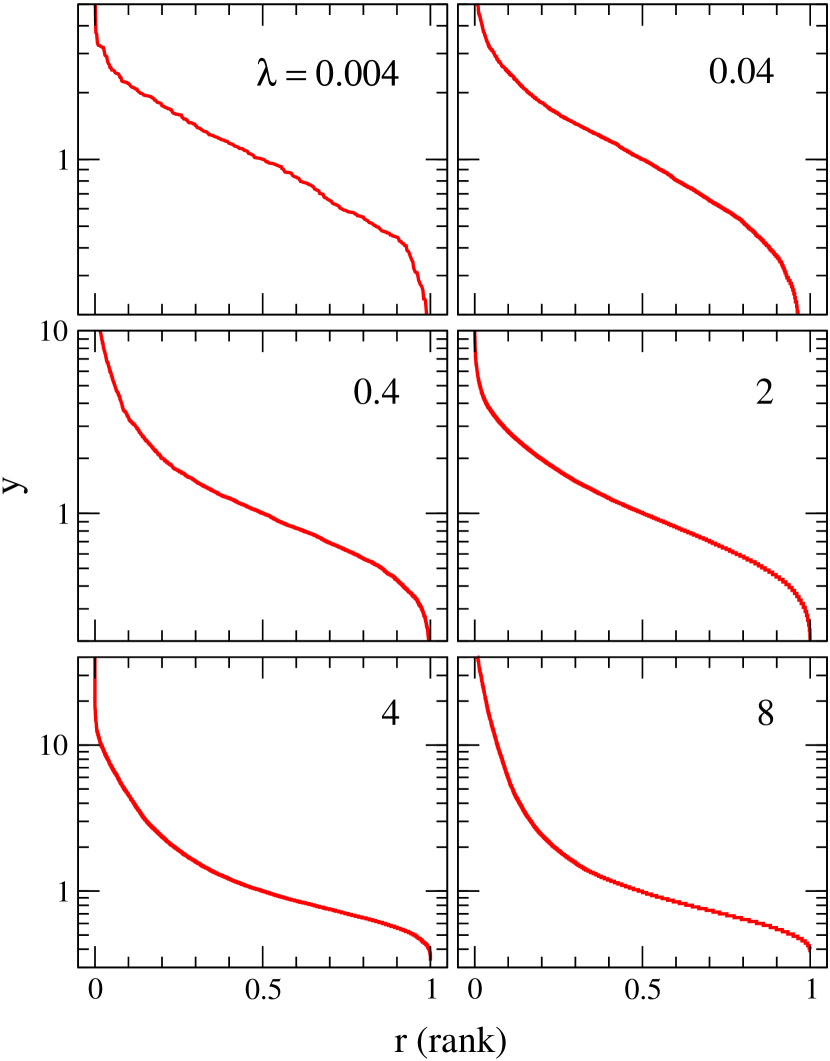
Figure 2: (Color online) Scaled rank-size distribution $y(\lambda,r)$ in semi-log scale for different values of competitiveness $\lambda$. These curves have been obtained by computing a large number of competitive processes to reduce statistic fluctuations.

3.2 Study and classification of empirical distributions by competitiveness

We have found that the change performed above to reduced unit $y$ can be applied to empirical data to compare the distributions for city sizes and electoral results in different countries or states. It allows to compare the effect of societal features, such as policies and economic data. Furthermore, a comparison between these distributions and those obtained via our simulations can be performed to assign a competitiveness value to the empirical data. This assignation is effected by minimizing the distance between the data and the computed curve $y(\lambda,r)$, using a Kolmogorov-Smirnof test KST (some examples are displayed in Fig. 3-Fig. 9 for electoral results and city populations). Since our simulation fits nicely the data, we are compelled to conclude that in general, the scaled distributions of city populations and electoral results can be classified according to the values of $\lambda$.

3.2.1 City size distributions

We have performed an exhaustive city-population study for the provinces of Spain muni . We have fitted each distribution to $y(\lambda,r)$ and have found a competitiveness distribution with a median of $\lambda_{1/2}=0.65$, reflecting some local dependence. We depict in Figs. 3 and 4 the scaled rank-size distributions of some provinces, together with the accompanying $\lambda$-family of distributions, which nicely fit the data. We have found that the rank-size distribution of the capital cities has a competitiveness of $0.71$ (Fig. 3f), which does not significantly differ from the median value. We contend that the fact that this distribution can be classified by competitiveness is a signature of the scale invariant nature of the social system: the whole country can be thought of as a single network of (only) capital cities, which displays similar statistical properties as those of the complete network, which includes all cities.

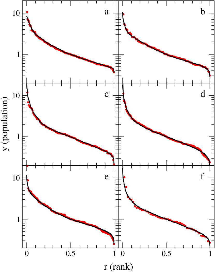
Figure 3: (Color online) Classification of city-size distributions by competitiveness ($\lambda$). a, scaled rank-plot of the city population of Girona province ($\lambda=1.74$) b, Bizkaia ($\lambda=1.63$) c, Castelló ($\lambda=0.65$) d, Cuenca ($\lambda=0.58$) e, Granada ($\lambda=0.06$) f, capital cities of Spanish provinces ($\lambda=0.71$). All empirical data are plotted with red dots, and compared to the rank-size distributions obtained with a numerical simulation employing the same value of competitiveness (in black lines).

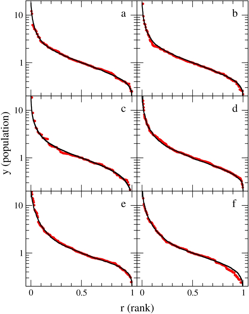
Figure 4: (Color online) Classification of city-size distributions by competitiveness ($\lambda$). a, scaled rank-plot of the city population of Tarragona province ($\lambda=0.69$) b, Cáceres ($\lambda=0.65$) c, Burgos ($\lambda=0.65$) d, Cantabria ($\lambda=0.59$) e, Ávila ($\lambda=0.43$) f, La Rioja ($\lambda=0.33$). All empirical data are plotted using red dots, and compared to the rank-size distributions obtained with our numerical simulation employing the same value of competitiveness (in black lines).

We have detected some singular exceptions in the fitting of these curves, as illustrated in Fig. 5 for the provinces of Guadalajara and Málaga. We understand that these deviations from the $\lambda$-family of distributions reflect local effects in policies or in social, economical or geographical factors, as some studies have found valitova . In the case of Guadalajara, the uppermost cities in the plot —those that deviate from the best fit— are located in the neighborhood of Madrid, the capital of Spain. The capital of Spain thus affects the population distribution in its neighborhood.

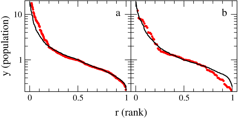
Figure 5: (Color online) Examples of deviations from the $\lambda$- family of distributions. a, scaled rank-plot of the city population of Guadalajara province, compared with the best fit. Deviations are seen in the case of the cities at the graph’s top (see text). b, Málaga, where the above deviations are also present. All empirical data are plotted using red dots, and simulation with black lines.

The empirical maximum degree $\hat{k}_{M}$, which defines the volume of the SFIN in configuration space, has been estimated for each province by solving the equation

$$\frac{\hat{k}_{M}}{\ln\hat{k}_{M}}=\lambda\frac{\hat{N}}{\hat{n}_{c}\hat{n}_{i}}.$$ (18)

Here $\hat{N}$ is the total population, $\hat{n}_{c}$ the number of cities and $\hat{n}_{i}$ the population of the smallest city, which is used to estimate the minimum cluster size. We have found that the empirical distribution of the maximum degree exhibits a large tail, whose median is $166$. The first and third quartiles are $37$ and $319$ respectively, hence

$$\langle\hat{k}_{m}\rangle=166^{+153}_{-129}.$$ (19)

We exhibit in Fig. 6 the competitiveness versus the empirical value of maximum degree of the Spanish provinces. The medians of both parameters are also shown.

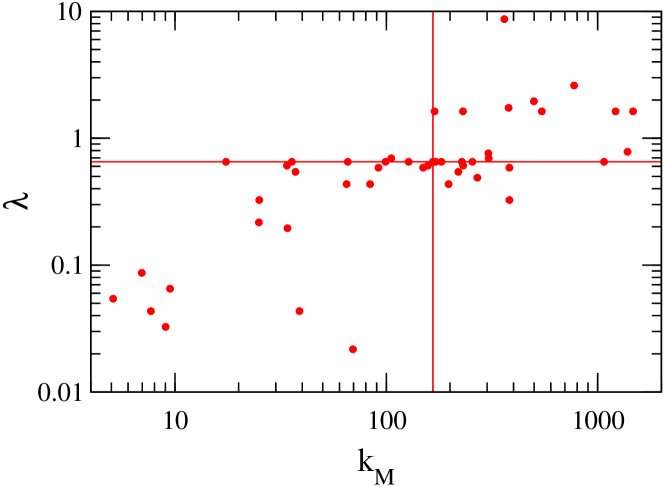
Figure 6: (Color online) Plot of the competitiveness $\lambda$ of the Spanish provinces versus the empirical value of maximum degree $k_{M}$. The medians of both parameters are represented by lines.

The maximum number of connections is an observable that has been evaluated before in the literature and is known as Dunbar’s number resdum . It can be found in the fields of anthropology, evolutionary psychology, and sociology. It reflects the fact that the maximum number of individuals with whom any person can maintain stable social relationships is determined by the size of their neocortex dunbar . Dunbar’s number lies between $100$ and $230$, but a commonly detected value is $150$, which fits quite well our results. As far as we know, the present work is the first in which Dunbar’s number is computed using a mathematical model based on first principles. We have checked with the case of the province of Teruel that a SFIN with a maximum degree of $150$ is able to reproduce the associated empirical distribution without the need of scaling it via the change to variable $y$. A total population of $109\,810$ inhabitants, excluding the capital city –we have already seen that the capital belongs to a larger national network–, distributed into $235$ cities, is modelled by a network of i) $N=100\,000$ nodes, ii) a maximum degree of $k_{M}=150$, and iii) by “growing” $n_{c}=250$ clusters with an initial size of $n_{i}=1$ node. We depict the rank size distribution in Fig. 7a, where it can be clearly seen that the simulation nicely fits the data. The city-size distribution is also compared with the cluster growth process obtained in a Barabasi-Albert network (BA) with the same number of nodes and clusters. In this figure we see that not all kinds of networks will be able to reproduce the empirical distribution, even if we employ a similar number of nodes and clusters, as in the case of the BA network.

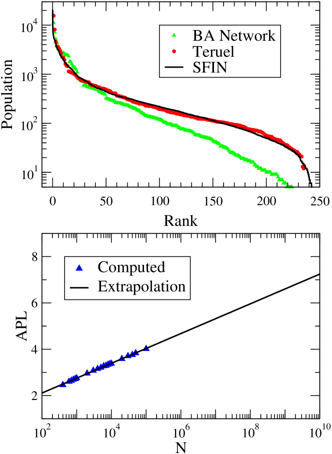
Figure 7: (Color online) Top panel, rank-size distribution of Teruel, Spain (red dots) is compared to the result of competitive processes carried out in networks with $N=100\,000$ nodes and where Dunbar’s number is the maximum degree, $k_{M}=150$ (black line). The size distributions are not scaled, which implies a relation one to one between inhabitants and nodes. We also show the result of the process in a BA network, which is not able to reproduce the empirical distribution (see text). Bottom panel, average path length —computed (blue dots) and extrapolated (black line)— for networks with maximum degree $k_{M}=150$. The extrapolation (see text) reproduces recent empirical measures.

The average path length (APL) of a network is defined, for all possible pairs of nodes, as the average number of steps along the shortest path. It is one of the most important quantities characterizing a network’s topology net1 . We have numerically computed the APL of a SFIN with $k_{M}=150$ as a function of $N$ up to $N=100\,000$ nodes. One easily sees the expected dependence on $\log N$, as illustrated by Fig. 7b. The extrapolation gives APL $=4.00$ for a SFIN of $100\,000$ nodes, APL $=5.63$ for $45\,000\,000$ nodes (population of Spain), APL $=6.13$ for $300\,000\,000$ nodes (population of the USA usa ), and APL $=6.95$ for $6\,500\,000\,000$ nodes (World population). These values are in accordance with the empirical measure of Travers and Milgram, known as the “six degrees” six , and with the more recent results of P.S. Dodds et al., who found an APL between $5$ and $7$ ele , or J. Leskovec and E. Horvitz, who found 6.6 degrees between Messenger users mess . These results indicate that the “six degrees of separation” is a direct consequence of Dunbar’s number.

3.2.2 Electoral results

We have carried out a similar competitiveness study for the results of General Elections in different countries and computed the $\lambda$ value in the cases of UK’05 elecUK , USA’04 elecUS , Italy’08 elecIt , and Spain’08 elecSp , finding $\lambda=6.5$, $4.6$, $2.7$, and $0.98$, respectively (Fig. 8), all values being larger than the average found for city populations. In general, a high value of the competitiveness increases the difference in the number of votes between two consecutive parties in the rank of results.

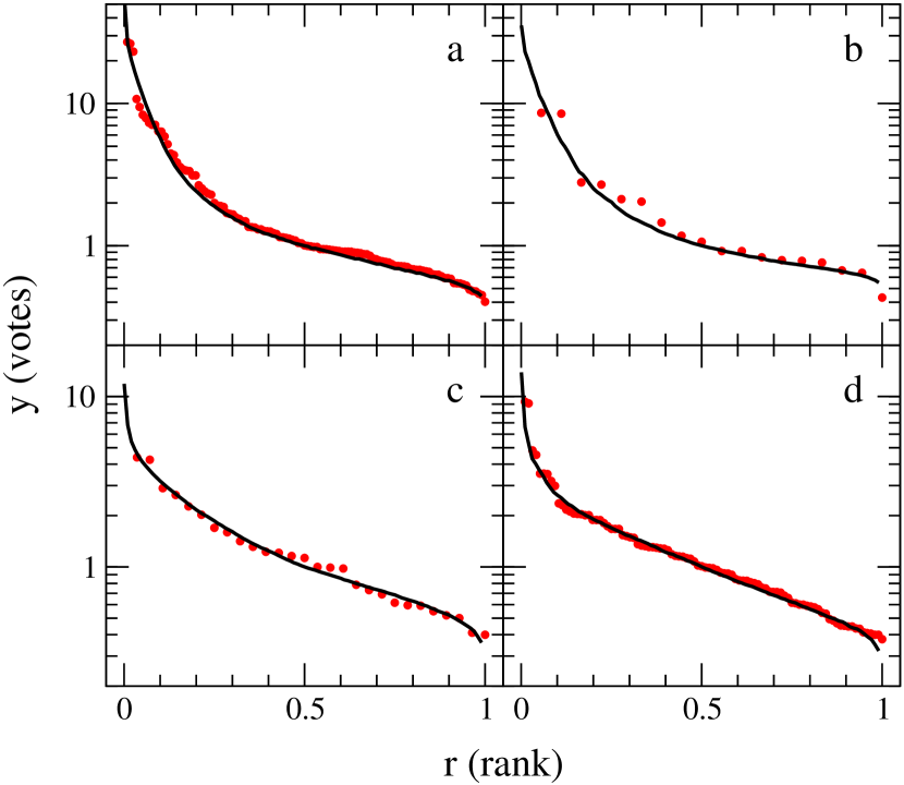
Figure 8: (Color online) Classification of electoral results distributions by competitiveness ($\lambda$). a, scaled rank-plot of the 2005 elections results in UK ($\lambda=6.5$). b, 2004 elections results in the USA ($\lambda=4.6$). c, 2008 elections results in Italy ($\lambda=2.7$). d, 2008 elections results in Spain ($\lambda=0.98$). All empirical data are plotted using red dots, and are compared to the rank-size distributions obtained via a simulation employing the same value of competitiveness (in black lines).

The estimates of the maximum degree are $\hat{k}_{M}\sim~{}600\,000$, $3\,000\,000$, $19\,000$, and $35\,000$, respectively, i.e., many orders of magnitude larger than Dunbar’s number. Thus, the volume in configuration space of the SFIN that describes the election process is larger than that for the city population. This is the effect of the creation and development of temporary connections. A politician, journalist, or blog writer can be easily connected during the electoral campaign to thousands of people via mass media, such as television, newspapers, or the Internet. In accordance with Dodds’ results, the world becomes smaller —more connected— when individual incentives exist ele , in this case to obtain good electoral results. These findings lead to interesting conclusions. In the USA’s case we find larger hubs than in the UK: $3\,000\,000$ connections against $600\,000$, but since the total population is $N_{p}=300\,000\,000$ against $61\,000\,000$ pobuk , the relative value is similar for each country, $\hat{k}_{M}/N_{p}\sim 0.01$. This value indicates that the USA and the UK have similar social networks in electoral campaigns, but scaled. Since there are more parties competing in elections in UK’s case, the distribution of the results naturally displays a higher competitiveness than in the USA’s one.

3.2.3 The universal distribution

Studying the city population of different countries around the world datospaises we have found that, for countries with a population over $5\,000\,000$, the main portion of the scaled distributions turns out to be quite similar, in fact the same distribution, thus evidencing some degree of universality, as illustrated in Fig. 9 for USA and Germany. Even the distribution of the size of companies in these countries follows this behavior, as depicted in the same figure for USA firms usa . This universal distribution can be reproduced by our simulation. Note that the competitiveness has a local dependence, and thus data of a country are in fact several sets of data (for many states or provinces of that country), which have different values of the competitiveness. We have simulated this universal distribution by mixing data generated with different values of competitiveness, between $0.4$ and $1$, obtaining the curve $y_{0}(r)$, which nicely fits the empirical distributions as can be seen in Fig. 9.

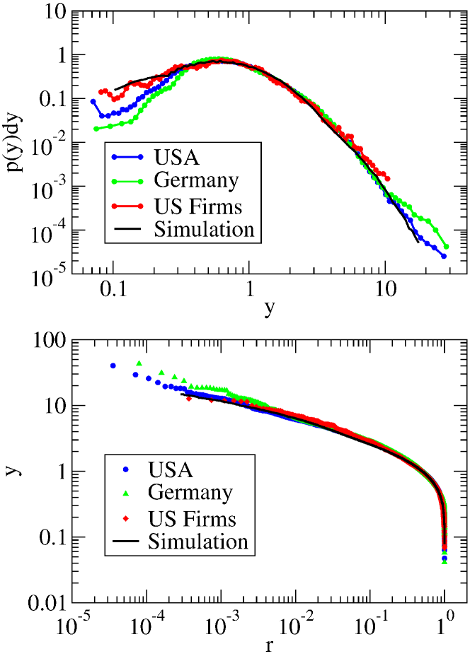
Figure 9: (Color online) Top panel, scaled city-size distribution for the USA (green squares) and Germany (blue triangles), and scaled firm-size distribution of the USA (red circles) compared to the universal distribution generated with our numerical simulation (black line) by mixing a large amount of data with different values of competitiveness. Bottom panel, same as top panel for the scaled rank-size distribution in log-log scale.

4 Summary and discussion

We have shown in this communication that the main properties of the city-size distributions and electoral results can be well reproduced when interactions between network elements are introduced by means of a competitive cluster growth process in a SFIN. We classify the deviations from the SFIN distribution in terms of just a single parameter, the competitiveness $\lambda$, that quantifies the strength of the interaction between the elements of the system. As expected, the SFIG-distribution emerges naturally in the limit of low competitiveness. The value of $\lambda$ can be easily extracted from empirical data by using the transformation to reduced units given in Eq. (11) and then comparing the scaled distribution to a distribution of known competitiveness.

In our simulations this parameter is related to the total density of clusters and to the maximum degree of the network —or the volume in the configuration space— by Eq. (17). For real systems, our results in the study of the Spanish provinces indicate that this relation remains valid. We have used it to compute the empirical average of the maximum degree, finding that it reproduces Dunbar’s number dunbar . Furthermore, the rank-size distribution of Teruel is reproduced using real values for the density of cities together with a maximum degree in a SFIN. Our simulations also predict the empirical estimate of the average path-length when we use Dunbar’s number for the maximum degree of the SFIN. This indicates that the known “six degrees of separation” six is a consequence of Dunbar’s number. For electoral results, we have found that the maximum degree grows by an order of magnitude —the volume in the configuration space grows—, which confirms the statement that the world is more connected when individual incentives do play a role.ele

Some studies have found correlations between city-size distribution and regional policies valitova . We believe that the use of the $\lambda$ parameter for such studies would add a very useful tool in order to classify the ensuing distributions. What could represent an advance in social and political sciences, would be to systematically assess the dependence of the competitiveness on local policies. As seen in the case of electoral results, a high value of the competitiveness enhances the difference (in number of votes) between two consecutive parties in the results rank. This implies that a small party would prefer a scenario with a low value of $\lambda$ in order to get better chances in the final tallies, whereas a big party would choose a high value in order to increase the relative difference with the other parties. For city sizes, a low value of the competitiveness works against supersaturated cities, whereas a high value promotes the importance of a capital city.

In general, all empirical distributions agree quite well with those obtained with our simulation, but we found also some singular exceptions. We expect these to be related to the already mentioned regional policies, and to historical or geographical factors. Thus, our model could help to identify such scenarios. Exhaustive studies of data around the world are necessary to build a bridge between the three variables of Eq. (14), $\rho_{s}$, $k_{m}$ and $\lambda$, and the social and economic polices of a region. It is also reasonable to think that a study in competitiveness terms of the evolution of firms-size distributions during the last years may lead to a deeper understanding of the present economic situation.

Summing up, our results show that scale invariant thermodynamics yields a useful framework for dealing with scale invariant phenomena. Its application to social sciences here has provided some deeper insight into the way humans build up a society. This work only represents a first step, and it is expected that subsequent studies will enhance the predictive power of the theory.

- (1) M. Batty, Science 319, 769 (2008).
- (2) A. Blank, S. Solomon, Physica A 287, 279 (2000). X. Gabaix, Y.M. Ioannides, Handbook of Regional and Urban Economics, Vol. 4 (North-Holland, Amsterdam, 2004); W. J. Reed, J. Regional Sci. 42, 1 (2002).
- (3) M.E.J. Newman, Contemp. Phys. 46, 323 (2005).
- (4) V. Pareto, Cours d‘Economie Politique (Droz, Geneva, 1896).
- (5) G.K. Zipf, Human Behavior and the Principle of Least Effort (Addison-Wesley, Cambridge, MA, 1949).
- (6) L.C. Malacarne, R.S. Mendes, E.K. Lenzi, Phys. Rev. E 65, 017106 (2001); M. Marsili, Yi-Cheng Zhang, Phys. Rev. Lett. 80, 2741 (1998).
- (7) R. L. Axtell, Science 293, 1818 (2001).
- (8) K. Paech, W. Bauer, S. Pratt, Phys. Rev. C 76, 054603 (2007); X. Campi and H. Krivine, Phys. Rev. C 72, 057602 (2005); Y. G. Ma et al., Phys. Rev. C 71, 054606 (2005).
- (9) C. Furusawa and K. Kaneko, Phys. Rev. Lett. 90, 088102 (2003).
- (10) I. Kanter and D.A. Kessler, Phys. Rev. Lett. 74, 4559 (1995).
- (11) M. E. J. Newman, Phys. Rev. E 64, 016131 (2001).
- (12) A. Hernando, D. Puigdomènech, D. Villuendas, C. Vesperinas, A. Plastino, Phys. Lett. A (to be published); arXiv:0908.0501v1 (2009).
- (13) R. Albert, A.L. Barabási, Rev. Mod. Phys. 2074, 2047 (2002). M.E.J. Newman, A.L. Barabasi, D.J. Watts, The Structure and Dynamics of Complex Networks (Princeton University Press, Princeton, 2006).
- (14) T. Maillart, D. Sornette, S. Spaeth, and G. von Krogh, Phys. Rev. Lett. 101, 218701 (2008).
- (15) R.N. Costa Filho, M.P. Almeida, J.S. Andrade, and J.E. Moreira, Phys. Rev. E 60, 1067 (1999).
- (16) A. Hernando, C. Vesperinas, A. Plastino, Physica A (to be published); arXiv:0908.0504v1 (2009).
- (17) R. Frieden, A. Plastino, A. R. Plastino, and B. H. Soffer, Phys. Rev. E 60, 48 (1999).
- (18) UrbanSim: http://www.urbansim.org, SLEUTH: http://www.ncgia.ucsb.edu/projects/gig/, DUEM: http://www.casa.ucl.ac.uk/software/duem.asp.
- (19) S. Fortunato, C. Castellano, Phys. Rev. Lett. 99, 138701 (2007).
- (20) M. Batty, Cities and Complexity: Understanding Cities Through Cellular Automata, Agent-Based Models, and Fractals (MIT Press, Cambridge, MA, 2005).
- (21) H. Gould and J. Tobochnik, An Introduction to Computer Simulation Methods: Applications to Physical Systems, 2nd Ed. (Addison-Wesley, 1996).
- (22) W. J. Reed, and B. D. Hughes, Phys. Rev. E. 66, 067103 (2002).
- (23) R. Albert, H. Jeong, A.L. Barabási, Nature 401, 130 (1999).
- (24) R. Guimerà, R.L. Danon, A. Díaz-Guilera, F. Giralt, A. Arenas, Phys. Rev. E 68, 065103(R) (2003).
- (25) J. Leskovec, E. Horvitz, arXiv:0803.0939v1 (2008).
- (26) B. R. Frieden and B. H. Soffer, Phys. Rev. E 52, 2274 (1995); B. R. Frieden, Physics from Fisher Information, 2nd Ed. (Cambridge Univ. Press, Cambridge, 1998); B. R. Frieden, Science from Fisher Information (Cambridge Univ. Press, Cambridge, 2004).
- (27) K. Christensen, H. Flyvbjerg, Z. Olami, Phys. Rev. Lett. 71, 2737 (1993); A. Mezhlumian, S.A. Molchanov, J. Stat. Phys. 71, 799 (1993); S. Zapperi, K. Baekgaard Lauritsen, H.E. Stanley, Phys. Rev. Lett. 75, 4071 (1995); A.A. Moreira, D.R. Paula, R.N. Costa Filho, J.S. Andrade, Phys. Rew. E, 73, 065101(R) (2006).
- (28) M. Batty, Nature 444, 592 (2006).
- (29) D.J. Watts, Six Degrees: The Science of a Connected Age, (Norton, New York, 2003); Small Worlds: The Dynamics of Networks Between Order and Randomness, (Princeton University Press, Princeton, 1999).
- (30) A. Clauset, C.R. Shalizi, M.E.J. Newman, arXiv:0706.1062v2 (2009).
- (31) National Statistics Institute of Spain website, Government of Spain, (www.ine.es).
- (32) L. Valitova, V. Tambovtsev, Regional policy priorities in Russia: empirical evidence. RECEP Reports, 5, 9 (2005).
- (33) M. Gladwell, The Tipping Point - How Little Things Make a Big Difference. (Little, Brown and Company, 2000).
- (34) R.I.M. Dunbar, J. Hum. Evo. 20, 469 (1992). Beh. Brain Sci. 16, 681 (1993).
- (35) Census bureau website, Government of USA, www.census.gov.
- (36) J. Travers, S. Milgram, Sociometry 32, 425 (1969).
- (37) P.S. Dodds, R. Muhamad, D.J. Watts, Science 301, 827 (2003).
- (38) Electoral Commission, Government of UK, http://www.electoralcommission.org.uk.
- (39) National Archives and Records Administration, Government of USA. www.archives.gov.
- (40) Ministero dell’Interno - Elezioni Politiche, Government of Italy. politiche.interno.it.
- (41) Ministerio del Interior, Elecciones, Government of Spain. www.elecciones.mir.es.
- (42) UK Statistics Authority, www.statistics.gov.uk.
- (43) Wolfram Mathematica CityData Source, based on a wide range of sources. www.wolfram.com.