Detailed maps of interstellar clouds in front of Centauri: Small-scale structures in the Galactic Disc–Halo interface
Abstract
The multi-phase interstellar medium (ISM) is highly structured, on scales from the size of the Solar System to that of a Galaxy. In particular small-scale structures are difficult to study and hence are poorly understood. We used the multiplex capabilities of the AAOmega spectrograph at the Anglo-Australian Telescope to create a half-square-degree map of the neutral and low-ionized ISM in front of the nearby ( kpc), most massive Galactic globular cluster, Centauri. Its redshifted, metal-poor and hot horizontal branch stars probe the medium-strong Ca ii K and Na i D2 line absorption, and weak absorption in the 5780 and 5797 Diffuse Interstellar Bands (DIBs), on scales around a parsec. The kinematical and thermodynamical picture emerging from these data is that we predominantly probe the warm neutral medium and weakly-ionized medium of the Galactic Disc–Halo interface, –1 kpc above the mid-plane. A comparison with Spitzer Space Telescope 24-m and DIRBE/IRAS maps of the warm and cold dust emission confirms that both Na i and Ca ii trace the overall column density of the warm neutral and weakly-ionized medium. Clear signatures are seen of the depletion of calcium atoms from the gas phase into dust grains. Curiously, the coarse DIRBE/IRAS map is a more reliable representation of the relative reddening between sightlines than the Na i and Ca ii absorption-line measurements, most likely because the latter are sensitive to fluctuations in the local ionization conditions. The behaviour of the DIBs is consistent with the 5780 band being stronger than the 5797 band in regions where the ultraviolet radiation level is relatively high, as in the Disc–Halo interface. This region corresponds to a -type cloud in which Ca i and small diatomic molecules such as CH and CN are usually absent. In all, our maps and simple analytical model calculations show in unprecedented detail that small-scale density and/or ionization structures exist in the extra-planar gas of a spiral galaxy.
keywords:
stars: horizontal branch – ISM: molecules – ISM: structure – Galaxy: disc – Galaxy: halo – globular clusters: individual: Cen (NGC 5139)1 Introduction
“Overhead the sky was full of strings and shreds of vapour, flying, vanishing, reappearing, and turning about an axis like tumblers, as the wind hounded them through heaven.” (Stevenson 1879). The interstellar medium (ISM) is indeed an extra-ordinarily dynamic place. Cooling and heating processes are continuously at work to transform gas between different states, from hot ionized gas with K visible in X-rays, to a cold neutral medium with K visible in H i and far-IR emission (Heiles & Troland 2005). The hotter media tend to fill space, whereas the colder media tend to form discrete structures (Cox 2005). The dynamics are important for Galactic recycling such as the re-accretion of gas from the Galactic Halo as fountains of hot gas from supernovae in the Galactic Disc cool and condense. They also influence the formation of small-scale structure in the form of filaments and small clumps, which must be transient features as they are out of pressure equilibrium with their surroundings (Stanimirović & Heiles 2005). Some of these structures have AU scales; we know very little about the 3D shapes of these tiny-scale structures, although a sheet-like geometry seems likely (Heiles & Troland 2005).
Absorption-line studies, e.g., against pulsars in radio or stars in optical/ultraviolet, can probe the small-scale structure; by using the relative proper motion of the background source, 1D tiny-scale structure can be traced (Heiles 1997; Crawford 2003). Mapping small- and tiny-scale structure directly is often limited by large separations between background sources, and limited angular resolution. Together with mapping high-surface brightness nebulae (e.g., Lazio et al. 2009), globular clusters offer some of the best possibilities for mapping experiments.
Langer, Prosser & Sneden (1990) observed several sightlines towards the globular clusters M 15 and M 92, finding evidence for significant column density and velocity variations on scales as small as 0.2 pc. Bates et al. (1995) presented similar findings for sightlines towards the globular cluster M 13. Variations on even smaller scales, down to pc, were detected towards globular clusters M 4 (Kemp, Bates & Lyons 1993) and the central parts of M 15 (Meyer & Lauroesch 1999) and M 92 (Andrews, Meyer & Lauroesch 2001). The latter team points out that fluctuations in ionization equilibrium and not total column density may be responsible for the observed variations. Points, Lauroesch & Meyer (2004) observed 150 sightlines towards the binary open cluster h & Persei, detecting both small-scale fluctuations as well as correlated behaviour over larger scales, suggesting variations in the physical conditions within sheets of gas.
We are incredibly fortunate to find ourselves in close proximity to Centauri, the most massive Galactic globular cluster ( M⊙; van de Ven et al. 2006). Few globular clusters are nearer to the Sun than Cen ( kpc; McDonald et al. 2009), resulting in a large number of suitable, bright probes of angular scales between an arcsecond and a degree — (sub)parsec scales in the intervening ISM. We here use its many horizontal branch (HB) stars. These stars are ideal probes: they are metal-poor, [Fe/H], and hot, K, and thus relatively clear of photospheric absorption in the interstellar lines of low excitation that probe the neutral and low-ionized ISM. The high retrograde velocity of Cen ( km s-1) moves the photospheric absorption out of the interstellar column. The proper motions of the stars are known too ( mas yr-1, van Leeuwen et al. 2000), so repeat observations may be used to probe the tiny-scale structure.
| Star | Equatorial coordinates | Galactic coordinates | E(B–V) | ——— Ca i K ———– | ——– Na i D2 ———– | 5780 | 5797 | ||||||
|---|---|---|---|---|---|---|---|---|---|---|---|---|---|
| (J2000) | (J2000) | ||||||||||||
| LEID | (deg) | (deg) | (deg) | (deg) | (mag) | (km/s) | (mÅ) | (mÅ) | (km/s) | (mÅ) | (mÅ) | (mÅ) | (mÅ) |
| 40004 | 201.06673 | 47.45981 | 308.669 | 15.0463 | 0.1301 | 19.4 | 28.6 | 5 | 13.6 | 22.7 | 4 | — | |
| 42009 | 201.11112 | 47.47200 | 308.698 | 15.0302 | 0.1304 | 32.1 | 30.3 | 5 | 13.2 | 23.0 | 4 | — | |
| 31006 | 201.12876 | 47.39312 | 308.721 | 15.1068 | 0.1256 | 24.3 | 29.6 | 5 | 13.4 | 23.6 | 3 | — | |
| 64010 | 201.18389 | 47.63934 | 308.726 | 14.8578 | 0.1417 | 27.9 | 32.2 | 6 | 16.5 | 26.2 | 5 | 3 | |
| 20006 | 201.14240 | 47.30854 | 308.743 | 15.1894 | 0.1227 | 17.8 | 27.2 | 4 | 12.1 | 22.6 | 3 | 4 | |
| 38008 | 201.18022 | 47.44549 | 308.750 | 15.0503 | 0.1286 | 25.4 | 29.9 | 5 | 17.3 | 27.0 | 5 | — | — |
| 26009 | 201.19651 | 47.35413 | 308.774 | 15.1393 | 0.1227 | 23.9 | 27.7 | 5 | 14.0 | 25.3 | 3 | 2 | |
| 35011 | 201.21149 | 47.42335 | 308.775 | 15.0694 | 0.1272 | 20.6 | 29.7 | 5 | 18.3 | 25.4 | 5 | — | |
| … | … | … | … | … | … | … | … | … | … | … | … | … | … |
The modest extinction, mag (McDonald et al. 2009), and Galactic latitude of Cen make the interstellar path towards Cen relatively simple. Yet several components have been identified, from the Local Bubble to a more distant spiral arm (Wood & Bates 1994). The interesting possibility is that some of the material we would probe could be in the Disc–Halo interface or associated with Cen itself; emission is seen at velocities of km s-1 in H i (McDonald 2009; McDonald et al., in prep.) and CO (Origlia et al. 1997). Absorption from the ISM in the 3968.47 & 3933.68 Å Ca ii H & K doublet was easily detected in 2dF spectra (van Loon et al. 2007)111Jones (1968) already noted the appearance of interstellar K-line absorption in the spectrum of the F-type giant Cen V1.. The same would be expected for the 5895.92 & 5889.95 Na i D1 & D2 doublet. The 2dF spectra were of too low a resolution to resolve the interstellar lines. We have since used its successor, AAOmega, at , to measure ISM features in 452 hot HB stars in Cen, of which we present the results here.
2 Observations
2.1 Spectroscopy with AAOmega
The observations were undertaken, in service mode, at the Anglo-Australian Telescope (AAT) on the night of 28 March 2008. The AAOmega spectrograph was used with the multiple-object-spectroscopy fibre feed from the 2dF fibre positioner (Saunders et al. 2004; Sharp et al. 2006).
The 5700 Å AAOmega dichroic was used. The red and blue arms of AAOmega were used with the 3200B and 2000R VPH gratings centered and blazed at 4040 Å and 5990 Å yielding spectra in the 3890–4170 Å and 5740–6220 Å regions at spectral resolutions (per 3.4-pixel resolution element) of ( km s-1) and ( km s-1), respectively. The exact ranges of individual spectra differ. The Ca ii H & K lines, which were the primary targets for the blue arm observations, were placed off centre on the CCD to avoid regions of poor cosmetic performance (bad columns). Skies were clear with seeing varying during the night from to ; the 2dF fibre entrances subtend on the sky.
Two fibre configurations were employed. Each observing block consists of a flat field frame (quartz-halogen lamp), an arc frame for wavelength calibration (CuAr, FeAr, He and Ne), a set of twilight sky flat field frames (to normalize the relative fibre transmissions for sky subtraction) and a series of 1800 second science frames. The total observing times for the two configurations sampling different stars were seconds and seconds, respectively.
The data were processed using the 2dfdr data reduction package. Two additional steps were performed under iraf prior to processing with 2dfdr. Firstly, a 2D bias frame was subtracted to correct a number of poor but recoverable columns in the data set. The 2D bias frame was created for this purpose from a stack of 30 bias frames via a -clipped mean rejection. Secondly, the iraf fixpix task was used to interpolate across a single bad column at the wavelength of the Ca ii K line. This isolated bad column affected the Ca ii K line in around 25% of spectra, with spectral curvature across the CCD moving it clear for the remaining stars. An updated bad-pixel mask was also created for 2dfdr to account for the effects of these modifications.
2dfdr performs the standard reduction operations: overscan correction; fibre trace and extraction; flat fielding and wavelength calibration. Cosmic ray rejection was applied to the 2D science frames by 2dfdr prior to extraction, following the prescription of van Dokkum (2001). In each configuration, 25 fibres were devoted to blank sky regions to create an average spectrum of the sky. Sky subtraction was performed using this sky spectrum. The relative intensity of the sky to subtract was determined from twilight flat-field frames obtained at the end of the night. Science frames were combined using a relative flux weighting derived from spectral intensities in each frame.
The spectra were not Doppler-corrected, i.e. they reflect the observer’s motion through space. All velocities used in this work and in the catalogue have been corrected to the Local Standard of Rest (LSR), though, by subtracting the km s-1 motion of the observer with respect to the LSR at the time of observation.
The continuum signal-to-noise ratio as measured on the extracted spectra is typically 30–50 per pixel around the Ca ii K line and 60–100 per pixel around the Na i D2 line.
2.2 Spectroscopic targets
Targets were selected from the proper motion catalogue of van Leeuwen et al. (2000). The criteria were designed to select blue stars, with mag and mag, that are likely members of Cen, with a membership probability % (all stars actually observed had %, and mostly 99 or 100%). A small number of targets were rejected due to close neighbours (), which would lead to contaminating light within the -diameter fibres. Hence 995 potential targets were available.
To maximise the uniformity and density of the area on the sky covered by our observations, targets were drawn from a field with radius and mutual separation . The bluest stars, with mag, were given priority, then stars with mag at , followed by stars with mag at and stars with mag at . We used the configure software with the simulated annealing method to configure the fields, and hence produced a second field with the leftovers from the first configuration. In all, 452 targets were observed in two field configurations.
To position the fibres accurately on sky, 6 and 7 fiducial stars were observed for the first and second configuration, respectively. These were chosen from amongst the brighter red giants, with mag and mag, with the same membership criterion as before to guarantee a good relative astrometric and fibre-positioning accuracy. The sky positions were chosen using the same target selection software, avoiding contamination within equivalent to mag in the fibre.
The observed stars are listed in Table 1, the full version of which is made available electronically; their locations in the B, B–V colour–magnitude diagram and on the sky are shown in Figs. 1 and 2, respectively.


3 Results

The average spectra in the blue and red regions are shown in Fig. 3. Besides the strong Balmer hydrogen absorption lines arising in the photospheres of the stars, the interstellar Ca ii H & K and Na i D1 & D2 lines are very obvious features observed with ease in every single spectrum. Two Diffuse Interstellar Bands (DIBs) are discernible in the red portion of the average spectrum, at 5780 and 5797 Å.
3.1 Interstellar Ca ii and Na i absorption
Average profiles of the Ca ii H & K and Na i D1 & D2 lines are shown in Fig. 4: the shorter-wavelength interstellar absorption lines of these multiplets, Ca ii K and Na i D2, are well isolated from their photospheric counterparts and are seen against a clean photospheric continuum; the weaker Ca ii H and Na i D1 lines are affected by strong photospheric Balmer H and photospheric Na i D2 line absorption, respectively. The kinematic offset between stars and ISM is small enough to avoid confusion with the 5875.6 Å He i D3 line.


The equivalent widths, line widths and central velocities of the interstellar Ca ii K and Na i D2 lines were measured by fitting a Gaussian (Table 1). This worked satisfactorily, the average result of which can be judged in Fig. 4. Note that the line width is given in terms of the value of the Gaussian, and hence is related to the Full-Width at Half Maximum as . This includes the contribution of the instrumental broadening, and km s-1 for the Ca ii K and Na i D2 lines, respectively. The formal errors on the velocities are a tenth of the spectral resolution element, or km s-1(222A check on the photospheric components reveals coincidence between Ca ii and Na i lines in Cen stars within a few km s-1.). The errors on the equivalent widths were derived from the standard deviation of the residuals of the Gaussian fitting, summed in quadrature and weighted by the Gaussian fit. Typical errors are 20–30 mÅ for the Ca ii K line and 15–20 mÅ for the Na i D2 line.
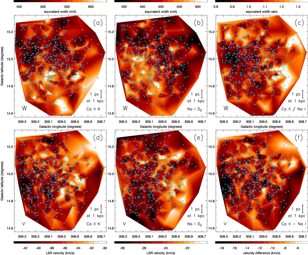
The equivalent widths in sightlines were then used to construct maps of the interstellar absorption as well as the line ratio (Fig. 5). The equivalent widths of both the Ca ii K and Na i D2 lines varied very significantly compared to the precision of the measurements, but by less than a factor two across the maps (Fig. 5a and b): mÅ (range 383–709 mÅ); mÅ (range 350–682 mÅ). The standard deviations in the distributions of and values are 48 and 63 mÅ, or 9% and 13%, respectively, compared to the mean errors in the equivalent width values of 25 and 15 mÅ, or 5% and 3%, respectively. The real fluctuations in the Ca ii K and Na i D2 maps thus amount to % and 12%, respectively.
The equivalent width values can be converted to column densities in the lower energy level of the transition, following van Dishoeck & Black (1989):
| (1) |
where the wavelength is in Å, the equivalent width is in mÅ, and the oscillator strengths are and 0.67 for the Ca ii K and Na i D2 lines, respectively. We thus obtain cm-2; cm-2. The conversion to column density assumes that the lines are weak enough to be on the linear part of the curve-of-growth. Given the moderate values for the equivalent width and reddening, E(B–V), this is not a bad assumption (see Crawford 1992a for examples of resolved line profiles at different E(B–V) values). It also assumes a single kinematic component, whereas in our case the absorption is a blend of at least two kinematically distinct components (see below).
Structure is visible on all scales, between neighbouring sightlines (but not always) as well as across the field. The atomic line ratio varied slightly more (Fig. 5c), (range 0.72–1.54), or (range 1.7–3.6). Indeed, although there are regions where the two lines vary in concert (e.g., the lower-left area and upper border in Fig. 5), there are regions where either the Ca ii K (e.g., the top-left corner and right border in Fig. 5) or the Na i D2 (Fig. 5: around , ) absorption is relatively strong.
The Na i D2 line is broader in wavelength than the Ca ii K line, but not in velocity: km s-1 (range 19–30 km s-1), whereas km s-1 (range 24–37 km s-1). Interestingly, the ratio of equivalent widths correlates significantly with that of the line widths (Fig. 6a, with Pearson’s values , ), and a corresponding shift in the central velocity between the two lines is seen (Fig. 6b, , ). This suggests that at least some sightlines pass through multiple absorption components (clouds), with Na0 clouds appearing at somewhat more positive velocities, and Ca+ clouds at more negative velocities. We will come back to this observation in the discussion section.

3.2 Diffuse Interstellar Bands

The first DIB features to have been found (Heger 1922) and shown to be of interstellar origin (Merrill 1934) are at 5780 and 5797 Å. The modest reddening towards our stellar probes not surprisingly results in rather weak DIB features, but in the average spectrum they are clearly detected at 4 and 2% depth with respect to the continuum (Fig. 7).
Gaussian fitting was on the whole still adequate, with typical errors of 20–40 mÅ for the 5780 DIB and 15–25 mÅ for the weaker but sharper 5797 DIB. Only fits of reasonable fidelity were kept by imposing a threshold on the equivalent width, mÅ, and constraining the bandwidth () to within 0.15–1.8 Å for the 5780 band and 0.15–1 Å for the 5797 band. Thus we kept the majority (415) of 5780 fits but only a third (164) of the 5797 fits. For these, the equivalent widths were mÅ, up to a maximum of 251 mÅ, with a bandwidth Å, and mÅ, up to a maximum of 128 mÅ, with a bandwidth Å. The shape of the 5797 band deviates from that of a Gaussian profile, not least due to a broader, shallower band at 5795 Å. Considering the weakness of the 5797 band in our spectra the Gaussian fitting is as accurate as any method.
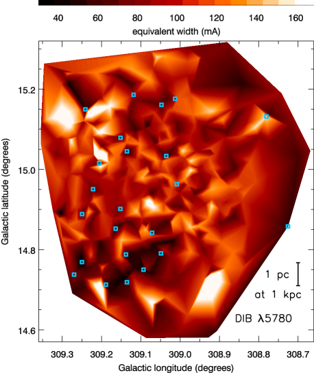
There are substantial variations of the DIB strength across the field and these are mapped in the stronger 5780 DIB in Fig. 8. This DIB is generally stronger where the Ca ii K line is weaker (compare Fig. 5). However, some strong 5780 absorption is seen in the upper left where the Na i D2 is weak but the Ca ii K line is not weak. Despite fewer sightlines the DIB map appears to have more small-scale structure, possibly because DIB absorption is generally associated with the neutral cloud medium which has a smaller filling factor than the warmer inter-cloud medium. However, much of the scatter is due to the uncertainties in the equivalent width measurements. The mean error in is 32 mÅ, whilst the standard deviation of the distribution of values (i.e. the fluctuations in the map) is 35 mÅ. Given the mean value for of 100 mÅ, this would suggest that the real fluctuations amount to “only” mÅ(15%), still comparable to — or exceeding — the fluctuations in Ca ii K and Na i D2.
A significant positive correlation exists for the ratio of 5780 DIB and Na i D2 equivalent widths and the ratio of Ca ii K and Na i D2 equivalent widths (Fig. 9b, , ; very small adjustments were made to the r-values to account for correlated errors in and ). This suggests that this DIB is strong where Ca+ is more abundant. There is no significant correlation between the ratio of 5780 DIB and Ca ii K equivalent widths and the Ca ii K/Na i D2 ratio (Fig. 9a, , ). There is no clear trend of the DIB ratio with Ca ii K/Na i D2 ratio either (Fig. 9c), but if the strongest -type absorption is selected (see below), , then these sightlines tend to be where the 5780 DIB is weak, but both Ca ii K and Na i D2 absorption are fairly strong (Figs. 5 & 8).

The ratio is an indicator of the ionization conditions as inferred from the atomic to total (H + H2) hydrogen ratio (Cami et al. 1997). The 5780 DIB is relatively weak in -Per type clouds and strong in -Sco type clouds (Krełowski & Sneden 1995), so the Disc–Halo interface region appears to be of type. The charge state of the 5780 and 5797 band carriers is not known, but if both are, for example, singly charged cations, then the low-UV () c.f. high-UV () classification is consistent with the parent neutrals having low (5797) and relatively high (5780) first photo-ionization energies such that the 5780 absorption appears when the UV field is strong. The -type character observed towards Cen is consistent with other observations of the 5797 and 5780 diffuse bands along sightlines out of the Galactic plane. Examples of observations of Milky Way diffuse band absorption are those seen towards the Magellanic Clouds (Ehrenfreund et al. 2002; Welty et al. 2006), and also SN 1987A (LMC) (Vladilo et al. 1987) and SN 1986G (NGC 5128) (D’Odorico et al. 1989) for which the reported ratios are 1/4 and 1/2, respectively.
The 6196 and 6203 DIBs are also seen in some of the spectra. However, this is close to the edge of our spectral range, and is in fact not covered in all spectra. In the spectra that do cover these bands, they are generally too faint to allow a meaningful analysis.
3.3 Evidence for gas associated with Centauri?
The spectral resolution element exceeds the internal velocity dispersion of the Cen cluster (e.g., van Loon et al. 2007), and the generally weak but present photospheric absorption in both the Ca ii H and K lines and the Na i D1 and D2 lines further limits searches for absorption components arising in the intra-cluster medium (ICM) within Cen. One could only hope to find very strong absorption in particularly hot stars, or, more sensitively, significantly displaced absorption because of the stellar peculiar velocity with respect to the cluster’s systemic velocity.
The average spectrum does not reveal any absorption in addition to the local interstellar components around the Sun’s velocity and photospheric components of the stellar probes in Cen (Fig. 4). If large variations were to occur in the ICM, then there might be a possibility to discover ICM components in individual spectra. However, the signal-to-noise ratio of the individual spectra is limited, and the resulting column density sensitivity is cm-2 for the Ca ii H and K and Na i D1 and D2 lines. No evidence was found for ICM at a level exceeding this. Assuming a uniform column density across a circular area of radius, this corresponds to a limit of M⊙ unless Na0 and Ca+ were to be grossly under-representative species. This estimate is consistent with the M⊙ from Spitzer maps of Cen (Boyer et al. 2008; McDonald et al. 2009), and reinforces evidence for efficient clearing of the cluster by interaction with the hot Halo (van Loon et al. 2009).
4 Discussion
4.1 Density, ionization, or dust depletion?
Are we probing density variations, or fluctuations in ionization and excitation equilibrium, e.g., due to variations in the interstellar radiation field? The Solar abundances of sodium and calcium are nearly identical, and hence the relative column densities of Ca+ and Na0 readily indicate the dust depletion and excitation/ionization conditions. Purely thermally-broadened lines of sodium and calcium are unresolved in our spectra. With a mean atomic weight of 23 and 40, respectively, the line width would be km s-1 even for a K plasma. Resolution of these lines therefore signifies the presence of multiple clouds along the sightline, rather than providing a means to estimate the gas kinetic temperature. Furthermore, the ionization state is likely to be dominated by the local strength of the interstellar radiation field, and thus electron density, neither of which are particularly well-constrained.
One may assume that the occupancies of the 3s and 4s states for the Na i D and Ca ii doublets are mostly related to the ionization state rather than a different degree of excitation of a particular atomic species. The relevant ionization potentials are as follows: Ca0, 6.11 eV; Ca+, 11.87 eV; Ca++, 50.91 eV; Na0, 5.14 eV; Na+, 47.29 eV. This means that in the warm ionized medium (significant energy density above 13.6 eV), neither Na0 nor Ca+ are the dominant species. Still, these lower ionization stages remain well populated and, given the high ionization potentials of the next higher stage (in both cases), should be fairly stable in their occupancy. In the cold neutral medium (with H2), Na0 is dominant but there is no Ca+. Therefore, no correspondence between Ca ii and Na i can be found in the cold neutral medium. In the warm neutral/weakly-ionized medium (atomic H), Ca+ is abundant, but perhaps more susceptible to variations in radiation field than Na0 given that both ionizations to Ca++ and recombinations to Ca0 are frequent (c.f. Crawford 1992b).
The strong Na i 8183+8195 Å doublet corresponds to the transition upwards from the next state, 3p, but our spectra do not include this line. The Ca i 4227 Å line corresponds to the equivalent transition to the Ca ii doublet but in the neutral phase, but this line is not covered by our spectra either. The 4227 Å line is extremely weak or absent in earlier 2dF spectra (Figs. 6 & 11 in van Loon 2002). Careful re-examination of the 2dF spectra of the few hundred hottest stars in van Loon et al. (2007) resulted in a detection rate of a few per cent at most, with equivalent widths not exceeding a few per cent of that of the Ca ii K line. Thus we have no direct means of constraining the Boltzmann-Saha distributions over the electronic energy levels.
4.1.1 Sodium and calcium as tracers of dust
Calcium is a highly refractive element and thus easily depleted from the gas phase onto dust grains, even in diffuse clouds. Sodium is much less affected, which allows a test to be made by comparing the Na i and Ca ii equivalent widths with the reddening, E(B–V).
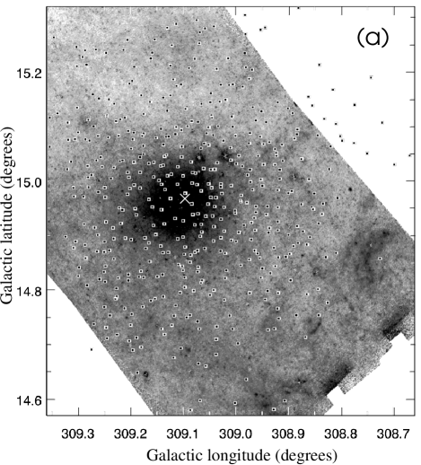
First we compare our absorption-line maps with the partly-overlapping Spitzer Space Telescope 24-m map (Fig. 10; c.f. Boyer et al. 2008). The latter shows starlight from the cluster in the central portion of the image, but mostly indicates where relatively warm dust is located. Focussing on the band of low 24-m surface brightness running from about , to about , , this is where the Na i absorption is weak but the ratio is fairly high. This suggests that we see warm material with little sign of calcium depletion, as expected in regions with little dust. Just below this band, around –, , lies of patch of dust emission; this is where Na i is strong and the ratio reaches the lowest values in our maps, suggesting high column densities of the neutral medium with strong calcium depletion.
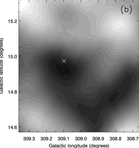
To better quantify the effects of depletion and test how well Na i traces the neutral medium, we correlate the equivalent widths with reddening values taken from the DIRBE/IRAS maps of cold dust (Schlegel, Finkbeiner & Davis 1998). These vary by % across the maps, between –0.144 mag; the reddening values are precise to 16% (Schlegel et al. 1998), although the statistical spread must be considerably smaller within the confines of this small portion on the sky (c.f. Fig. 10b). In spite of the vastly different angular resolution, the reddening map (Fig. 10b) reveals clear parallels with the Spitzer 24-m map (Fig. 10a). For instance, there is a dense cloud stretching across the lower-right corner, and a general lack of dust in the top part of the region. Curiously, the reddening map suggests a dust cloud very near (but just below) the centre of Cen. This might have been affected by far-IR starlight from the cluster, but the Na i absorption (in particular) is also rather strong in that patch of sky (Fig. 5).

The clearest correlation with E(B–V) is for Na i (Fig. 11a, , ), which increases in strength by at least %. This confirms that Na i indeed traces the column density of the neutral dusty medium (Hobbs 1974). The fact that it seems to increase more strongly than the reddening does, can most simply (and hence plausibly) be explained by a need to re-adjust the reddening values from the Schlegel et al. (1998) maps towards lower values. Indeed, the mean mag is mag higher than deduced from accurate analysis of the colour–magnitude diagram of stars within Cen (McDonald et al. 2009). If the correction is a simple offset, leaving the spread intact, then the reddening would vary by more than 20%, possibly by about 40% just as the Na i line strength does. Although McDonald et al. (2009) constrain differential reddening gradients across the cluster to mag near the cluster centre, Calamida et al. (2005) inferred reddening variations up to a factor almost two from the colours of hot HB stars in Cen, indicating a clumpy medium; given that the Schlegel et al. maps have a rather coarse resolution some of the spread in the Na i line strength may be due to such clumps.
The ratio shows a weak anti-correlation with E(B–V), at the % level (Fig. 11b, , ), consistent with the effects of dust depletion. However, given that the Na i line strengthens even more, it means that the Ca ii still appears generally stronger along dustier sightlines and therefore, to some extent, also traces the column density of the neutral medium (c.f. Hobbs 1974).

To test whether the Na i or Ca ii lines could be used to trace the small-scale distribution of interstellar dust, we deredden the B, B–V diagram using the DIRBE/IRAS maps, and again using instead a scaling of the reddening with the Na i and Ca ii equivalent width (Fig. 12). We parameterised and , and assumed .
Remarkably, the coarser DIRBE/IRAS map is much better in dereddening the colour–magnitude diagram than the absorption lines, despite the latter being observed along exactly the same sightlines as the stars that are being corrected. The clearest evidence for this statement is that the scatter in the HB sequence increases significantly when using the absorption lines, whereas it remains as tight as the original, observed sequence when using the DIRBE/IRAS maps. The errors in the equivalent width are typically %, translating into errors in E(B–V) and AB of and mag, respectively, i.e. smaller than the increased scatter. The increased scatter, especially when using the Na i absorption, would tend to imply that the variations arise from fluctuations in ionization equilibrium rather than total atomic column density, assuming that the atomic column densities are well correlated with dust. In any case it confirms that the fluctuations in the Ca ii K and Na i D2 lines are a physical reality.
4.1.2 The Diffuse Interstellar Bands
The 5780 and 5797 DIBs are encountered in diffuse clouds, with the 5780 DIB appearing stronger where the UV radiation field is stronger (-type clouds) — which presumably leads to the destruction of the carrier of the 5797 DIB which is stronger in denser neutral media (-type clouds) (Krełowski & Westerlund 1988; Krełowski et al. 1999). If both are singly-charged macromolecules, then their different UV threshold for appearance might be related to differences in the photo-ionization energy of their parent neutral molecules, that of the 5780 Å DIB being higher (c.f. Cami et al. 1997). Alternatively, it might simply reflect a difference in charge, with the 5780 DIB due to a weakly ionized or protonated macromolecule and the 5797 DIB due to a neutral macromolecule, much like the variations suggested in the mid-IR spectra of Polycyclic Aromatic Hydrocarbons (Allamandola, Tielens & Barker 1989).
The sightlines we probe here would be more translucent than in the Galactic plane, and hence the behaviour would be expected to dominate. Indeed, few sightlines in our data have a strong 5797 DIB, consistent with a low filling factor of the cold neutral medium. The highest ratios are seen where the 5780 band is weak not because the 5797 band is strong (Fig. 8). But more typically, it is the 5797 band which varies: in Fig. 13 two spectra are compared, showing weak and strong 5797 bands for very similar bands and Ca ii and Na i lines. The former is an average of the spectra of LEID 33137, 37193, 40185, 41087, 42153, 64042 and 75026, whilst the latter is an average of the spectra of LEID 20006, 21022, 26096, 55048, 60020 and 68026.


The 5780 DIB shows no correlation with E(B–V) over the small range in E(B–V) probed here. Comparing with the 24-m map (Fig. 10a) there is some correspondence between the absence of warm dust around , and stronger 5780 DIB absorption, and between the warm dust emission around , – and weaker 5780 DIB absorption. In the latter region the 5797 DIB is often seen, confirming the presence of a dense medium there. There are about ten times more sightlines with than with , which suggests that the denser medium traced by the 5797 DIB has a lower filling factor than the warmer neutral medium by a factor .

The gradient in reddening can help pinpoint the edges of clouds, under the assumption that the reddening reaches a maximum in the cloud core and a minimum in the inter-cloud regions. The (absolute value of the) gradient would be maximum near the boundary between cloud and inter-cloud region. There is a very tentative indication that at the steepest gradients, mag deg-1, the 5780 DIB is stronger than at shallower gradients (Fig. 14): mÅ versus mÅ, a difference of mÅ or 3 . A positive correlation, if significant, would be consistent with the 5780 DIB originating in the warmer envelopes of diffuse clouds.
4.2 The interstellar path towards Centauri
Much of the structure might be relatively near to us, seen against a smoother, more distant background higher above the Galactic Disc. Mapping of the nearby ISM indeed suggests that the path towards Cen first traverses the warm/hot gas of the Local Bubble until pc, then passes through a neutral medium until pc before leaving the Disc (Lallement et al. 2003). Although Cen is not seen through the bright H emission of the Galactic Disc, it is seen through a layer of fainter, more diffuse H emission (Gaensler et al. 2008) possibly associated with an extra-planar warm ionized medium. Given that Na i and Ca ii both trace the warm neutral medium one might have expected that the absorption bears a prominent imprint of the slab of neutral cloud material.
This does not appear to be the case. The column density ratio –3.4. For warm, inter-cloud material, Crawford (1992b) found that . In our case this would suggest that –0.12, i.e. a depletion of calcium by a factor . The ratios observed here suggest clouds of K and (probably within an order of magnitude) cm-1, also on the basis of calculations by Bertin et al. (1993), which is typical of the warm ionized medium.
Wood & Bates (1993, 1994) and Bates et al. (1992) have probed the ISM in front of, and surrounding, Cen with a few dozen stellar probes at distances from pc to kpc. They identified four main kinematic components which are also spatially distinct: (i) absorption around zero km s-1 arising from hot gas in the Local Bubble; (ii) absorption around km s-1 arising from cooler material between the Local Bubble and the expanding Scorpius-Centaurus shell; (iii) strong absorption around km s-1, associated with IR emission seen in IRAS maps, in a vertical extension of the Carina-Sagittarius spiral arm at –2 kpc distance from the Sun, and (iv) weaker and patchier absorption at more negative velocities, typically km s-1, arising from extra-planar gas beyond the Carina-Sagittarius arm, at pc above the Disc. If most of the absorption seen in the Ca ii K and Na i D2 lines is around 1–2 kpc distance then we probe scales of –20 pc.
The mean velocity of the Ca ii K line is km s-1. This suggests that the Ca ii K line originates predominantly in the extra-planar gas at a few kpc distance, either because it is warmer there or because dust depletion diminishes the Ca ii K line closer to us. The mean velocity of the Na i D2 line is km s-1. The Na i D2 line thus appears to arise predominantly in the puffed-up spiral arm at 1–2 kpc distance. This picture is confirmed by the fact that the more negative velocity seen in the Ca ii K line compared to the Na i D2 line occurs where the Ca ii K line is broader, the ratio is higher and the reddening is lower.
The kinematic lag observed in the extra-planar gas may not just be due to the projection of Galactic rotation. Gas infalling from the Halo will lag behind the Galactic rotation (Albert et al. 1993; Shull et al. 2009). Crawford et al. (2002) performed a detailed study in the Ca ii K and Na i D2 lines, but at much higher spectral resolution, of similar warm gas in the lower Halo seen through the Local Interstellar Chimney. They found evidence of cooling gas precipitating onto the Disc. Alternatively, drag experienced in the Disc–Halo interaction zône where the rotating gaseous Disc meets the hot Halo gas might slow down rotating extra-planar gas. Such interaction might also give rise to instabilities in the Disc, resulting in a spiral density wave, much akin to the standing sound waves generated when rubbing a metal pipe.
To investigate the possible presence of a velocity lag, we computed the line profile analytically, from:
| (2) |
where the optical depth is described as a function of distance to the Galactic Centre, , and the Galactic plane, , in a double exponential form:
| (3) |
where and are the Disc scalelength and scaleheight, respectively, and is the distance from the Sun.
The analytical expression for assuming a flat rotation curve, , and some of the derived quantities, are discussed in Appendix A. There, we also describe the more ungainly but still analytical result for the case where we introduce a velocity lag as a function of (“drag”):
| (4) |
where sets the rate of linear decline in the velocity. We assumed a distance to the Galactic Centre of kpc, km s-1 (c.f. Shattow & Loeb 2009), and kpc. The results are visualized in Fig. 15, compared to the observed Ca ii K line.
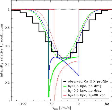
The model with kpc (c.f. Gaensler et al. (2008), for the warm ionized medium) peaks at too negative a velocity. The peak shifts to a more positive velocity if the scaleheight is lowered, or if some drag is introduced. The negative-velocity wing of the line profile shifts more in the latter case. Our average spectrum of the Ca ii K line is marginally more consistent with a lower scaleheight without the need to invoke drag. On the other hand, the most negative component in the higher resolution spectra presented in Bates et al. (1992) peaks at km s-1, which is exactly where a model peaks that has a moderate amount of drag ( kpc). In that model, this velocity extremum is reached at kpc, i.e. just in front of Cen (assumed to be at kpc).
4.3 Extra-planar small-scale ISM structure
As concluded in the previous section, our view towards Cen seen through the eyes of the Ca ii and Na i lines and 5780 and 5797 DIBs mostly shows the spiral arm–Halo interface and the extra-planar gas beyond it. Although we see neutral atomic and molecular gas, as well as dust depletion, that portion of the Disc–Halo interaction region has a prominent component of warm ionized gas, with a scaleheight of kpc and a filling factor of % (Gaensler et al. 2008) — note that Cen is 1.3 kpc above the Galactic plane. The hot corona permeating the Halo, making up most of the remaining 70% in volume, is not probed here.
Even though the ISM is a dynamic environment in which pressure equilibrium is unlikely to be strictly valid, it is largely the case that the volume filling factor of an ISM phase matches its temperature, following the equation of state (with the mean molecular weight). Cold media are found in the form of compact structures, with a high density (exacerbated by the lower temperature). But as the cross-section of such structures decreases, it is harder to sample the colder medium by means of discrete sightlines (as opposed to full imaging). Furthermore, superposition of separate cold structures is likely if the column length is substantial. Variations in column density across the sky should be reflected in variations along the sightline.
We have performed a simplistic analytical modeling attempt to assess the small-scale structure of the extra-planar neutral and low-ionized medium. This assumes a size distribution of spherical clouds of radii , between and :
| (5) |
with the specific density postulated by
| (6) |
The normalisation of the size distribution is obtained from
| (7) |
where is the volume filling factor for a rectangular volume of space, . In Appendix B we describe the derivation from this of the expected relative fluctuations in column density, . For reasonable assumptions of the parameters upon which this depends (see Appendix B), one would expect –0.2, and this is entirely consistent with the fluctuations we see in our maps. This once more confirms that we detect pc-scale structure in the neutral and low-ionized extra-planar gas.
We can not ascertain whether the extra-planar small-scale structure originates in the Galactic Disc and simply persists as gas migrates to higher elevations, or whether it is generated in situ, as a result of thermal instabilities in cooling gas. The latter may be associated with gas raining down from outflows generating within the “Galactic Fountain” paradigm (Shapiro & Field 1976; Spitzer 1990) — c.f. Crawford et al. (2002) for recent evidence of this scenario. Alternatively, it may drizzle down from much further afield (e.g., Stanimirović et al. 2006; Bland-Hawthorn et al. 2007).
5 Conclusions
Medium-resolution spectra of 452 blue-Horizontal Branch stars in the globular cluster Centauri were obtained, with the aim to determine the spatial and thermodynamical structure of the intervening diffuse interstellar medium. The study presented here is based on the Ca ii K and Na i D2 lines and the diffuse interstellar bands at 5780 and 5797 Å, which probe mainly the warm neutral and weakly-ionized medium. Maps were created spanning , showing fluctuations in all these tracers, up to a factor two in the Ca and Na lines, on all scales down to a few arcminutes. These fluctuations were reproduced in a statistical sense adopting a simple analytical model for a population of clouds with power-law distributions over size and density. Correlations with reddening confirmed that calcium depletion onto dust grains occurs in neutral clouds. The location of the Ca K and Na D dominant line-forming regions was deduced, on the basis also of kinematical evidence (line centroids and line widths) in agreement with literature high-resolution studies of a small number of sightlines.
The most pertinent conclusions of our investigation can be summarised as follows:
-
In the direction towards Centauri, , the Ca K and Na D lines and the 5780 and 5797 Å DIBs trace predominantly the neutral and weakly-ionized medium in the extra-planar Disc–Halo interface. The neutral medium is relatively more prominent in the front of this extended region, pc above the nearby (1–2 kpc) Carina-Sagittarius spiral arm, whilst the ionized medium dominates behind it, –1 kpc above the Galactic plane.
-
The extra-planar gas is dominated by -type clouds, in which the macromolecules held responsible for the DIBs are electrically charged. The 5780 Å DIB is identified with such carrier; it also appears stronger in the envelopes of neutral clouds, i.e. in the contact interfaces with warm gas, whilst the 5797 Å DIB is stronger within neutral clouds. This is consistent with the 5797 Å DIB being associated, either with a neutral carrier molecule or with a singly-charged cation at a lower photo-ionization threshold of the parent neutral molecule.
-
Small-scale structure is detected in both the neutral and weakly-ionized medium, down to scales of pc. This implies that small-scale structure persists — or is generated — well above the Galactic plane, several hundreds of pc (or more) away from the nearest sites of supernovae.
Acknowledgments
Jacco wishes to thank Snežana Stanimirović for inspiration that started this project. We are grateful for a service time award for AAOmega on the AAT. We would also like to thank the referee, Ian Crawford, for his constructive and valuable remarks. KTS thanks EPSRC for a studentship.
References
- [Albert et al.(1993)] Albert C.E., Blades J.C., Morton D.C., Lockman F.J., Proulx M., Ferrarese L. 1993, ApJS, 88, 81
- [Allamandola, Tielens & Barker (1989)] Allamandola L.J., Tielens, A.G.G.M., Barker J.R. 1989, ApJS, 71, 733
- [Andrews, Meyer & Lauroesch (2001)] Andrews S.M., Meyer D.M., Lauroesch J.T. 2001, ApJ, 552, L73
- [Bates et al.(1992)] Bates B., Wood K.D., Catney M.G., Gilheany S. 1992, MNRAS, 254, 221
- [Bates et al.(1995)] Bates B., Shaw C.R., Kemp S.N., Keenan F.P., Davies R.D. 1995, ApJ, 444, 672
- [Bland-Hawthorn et al.(2007)] Bland-Hawthorn J., Sutherland R., Agertz O., Moore B. 2007, ApJ, 670, L109
- [Bertin et al.(1993)] Bertin P., Lallement R., Ferlet R., Vidal-Madjar A. 1993, A&A, 278, 549
- [Boyer et al.(2008)] Boyer M.L., McDonald I., Loon J.Th., Woodward C.E., Gehrz R.D., Evans A., Dupree A.K. 2008, AJ, 135, 1395
- [Calamida et al.(2005)] Calamida A., et al. 2005, ApJ, 634, L69
- [Cami et al.(1997)] Cami J., Sonnentrucker P., Ehrenfreund P., Foing B.H. 1997, A&A, 326, 822
- [Cox (2005)] Cox D.P. 2005, ARA&A, 43, 337
- [Crawford (1992a)] Crawford I.A. 1992a, MNRAS, 254, 264
- [Crawford (1992b)] Crawford I.A. 1992b, MNRAS, 259, 47
- [Crawford (2003)] Crawford I.A. 2003, Ap&SS, 285, 661
- [Crawford et al.(2002)] Crawford I.A., Lallement R., Price R.J., Sfeir D.M., Wakker B.P., Welsh B.Y. 2002, MNRAS, 337, 720
- [D’Odorico et al.(1989)] D’Odorico S., di Serego Alighieri S., Pettini M., Magain P., Nissen P.E., Panagia N. 1989, A&A, 215, 21
- [Ehrenfreund et al.(2002)] Ehrenfreund P., et al. 2002, ApJ, 576, L117
- [Gaensler et al.(2008)] Gaensler B.M., Madsen G.J., Chatterjee S., Mao S.A. 2008, PASA, 25, 184
- [Heger (1922)] Heger M.L., 1922, Lick Obs. Bull., 10, 146
- [Heiles (1997)] Heiles C., 1997, ApJ, 481, 193
- [Heiles & Troland (2005)] Heiles C., Troland T.H. 2005, ApJ, 624, 773
- [Hobbs (1974)] Hobbs L.M., 1974, ApJ, 191, 381
- [Jones (1968)] Jones D.H.P. 1968, MNRAS, 140, 265
- [Kemp, Bates & Lyons (1993)] Kemp S.N., Bates B., Lyons M.A. 1993, A&A, 278, 542
- [Kim et al.(2007)] Kim S., et al. 2007, ApJS, 171, 419
- [Krełowski & Sneden (1995)] Krełowski J., Sneden C. 1995, in: The Diffuse Interstellar Bands, eds. A.G.G.M. Tielens & T.P. Snow, ASSL, Vol. 202 (Kluwer: Dordrecht), p13
- [Krełowski & Westerlund (1988)] Krełowski J., Westerlund B.E. 1988, A&A, 190, 339
- [Krełowski et al.(1999)] Krełowski J., et al. 1999, A&A, 347, 235
- [Lallement et al.(2003)] Lallement R., Welsh B.Y., Vergely J.L., Crifo F., Sfeir D. 2003, A&A, 411, 447
- [Langer, Prosser & Sneden (1990)] Langer G.E., Prosser C.F., Sneden C. 1990, AJ, 100, 216
- [Lazio et al.(2009)] Lazio T.J.W., Brogan C.L., Goss W.M., Stanimirović S. 2009, AJ, 137, 4526
- [McDonald (2009)] McDonald I. 2009, PhD thesis, Keele University
- [McDonald et al.(2009)] McDonald I., et al. 2009, MNRAS, 394, 831
- [Meyer & Lauroesch (1999)] Meyer D.M., Lauroesch J.T. 1999, ApJ, 520, L103
- [Merrill (1934)] Merrill P.W. 1934, PASP, 46, 206
- [Origlia et al.(1997)] Origlia L., Gredel R., Ferraro F.R., Fusi Pecci F. 1997, MNRAS, 289, 948
- [Points, Lauroesch & Meyer (2004)] Points S.D., Lauroesch J.T., Meyer D.M. 2004, PASP, 116, 801
- [Saunders et al.(2004)] Saunders W., et al. 2004, SPIE, 5492, 389
- [Schlegel, Finkbeiner & Davis (1998)] Schlegel D.J., Finkbeiner D.P., Davis M. 1998, ApJ, 500, 525
- [Shapiro & Field (1976)] Shapiro P.R., Field G.B. 1976, ApJ, 205, 762
- [Sharp et al.(2006)] Sharp R.G., et al. 2006, SPIE, 6269E, 14
- [Shattow & Loeb (2009)] Shattow G., Loeb A. 2009, MNRAS, 392, L21
- [Shull et al.(2009)] Shull J.M., Jones J.R., Danforth C.W., Collins J.A. 2009, ApJ in press
- [Spitzer (1990)] Spitzer, L.Jr. 1990, ARA&A, 28, 71
- [Stanimirović & Heiles (2005)] Stanimirović S., Heiles C. 2005, ApJ, 631, 371
- [Stanimirović et al.(2006)] Stanimirović S., et al. 2006, ApJ, 653, 1210
- [Stevenson (1879)] Stevenson R.L. 1879, “Travels with a donkey”
- [van de Ven et al.(2006)] van de Ven G., van den Bosch R.C.E., Verolme E.K., de Zeeuw P.T. 2006, A&A, 445, 513
- [van Dishoeck & Black (1989)] van Dishoeck E.F., Black J.H. 1989, ApJ, 340, 272
- [van Dokkum (2001)] van Dokkum P.G. 2001, PASP, 113, 1420
- [van Leeuwen et al.(2000)] van Leeuwen F., Le Poole R.S., Reijns R.A., Freeman K.C., de Zeeuw P.T. 2000, A&A, 360, 472
- [van Loon (2002)] van Loon J.Th. 2002, in: Omega Centauri, A Unique Window into Astrophysics, eds. F. van Leeuwen, J.D. Hughes & G. Piotto, ASPC, 265, 129
- [van Loon et al.(2007)] van Loon J.Th., van Leeuwen F., Smalley B., Smith A.W., Lyons N.A., McDonald I., Boyer M.L. 2007, MNRAS, 382, 1353
- [van Loon et al.(2009)] van Loon J.Th., Stanimirović S., Putman M., Peek, J.E.G., Gibson S.J., Douglas K.A., Korpela E.J. 2009, MNRAS, in press
- [Vladilo et al.(1987)] Vladilo G., Crivellari L., Molaro P., Beckman J.E. 1987, A&A, 182, L59
- [Welsh, Wheatley & Lallement (2009)] Welsh B.Y., Wheatley J.M., Lallement R. 2009, PASP, submitted
- [Welty et al.(2006)] Welty D.E., Federman S.R., Gredel R., Thorburn J.A., Lambert D.L. 2006, ApJS, 165, 138
- [Wood & Bates (1993)] Wood K.D., Bates B. 1993, ApJ, 417, 572
- [Wood & Bates (1994)] Wood K.D., Bates B. 1994, MNRAS, 267, 660
Appendix A Computation of line profiles with and without drag
To compute a line profile (Eq. (2)), we need to assess the optical depth in a velocity interval. This is related to the column density, and thus obtained from
| (8) |
In our application, the precise value of is not important so we scale it to match the observed line profile. The density, , as a function of distance to the Galactic Centre, , and Galactic plane, , is described in our model by a double exponential (c.f. Eq. (3)). The main mathematical exercise is to prescribe , , and distance as a function of .
Trigonometry relates and :
| (9) |
and and :
| (10) |
where and are the Galactic coordinates of the sightline. Further simple trigonometry yields a prescription for the radial velocity difference as a function of (and thus of ):
| (11) |
where and are the Galactic rotation velocities of the gas cloud and the Sun, respectively. For a flat rotation curve, , the distance at which the velocity difference reaches an extremum is given by
| (12) |
For the sightline towards Cen, , and adopting kpc and km s-1, one obtains kpc and a corresponding km s-1.
To obtain a prescription for , we need to invert Eq. (A4) (incorporating Eq. (A2)). For the case of a flat rotation curve this is straightforward:
| (13) |
where we introduce for the sake of brevity:
| (14) |
The plus/minus sign in Eq. (A6) arises from the fact that beyond the velocity evolves back towards zero, resulting in two solutions for the distance at any given velocity. In our situation, this is avoided by us only tracing gas up to the distance of Cen, which is just before the turning point . Hence, in our case the minus sign applies to Eq. (A6). The derivative is also readily derived, irrespectively of the sign:
| (15) |
The situation becomes more laborious if we replace the flat rotation curve by the modification following Eq. (4), to allow for some kind of drag between the Disc rotation and the Halo. However, the choice of this form still allows an analytical solution to be obtained, viz. for the distance:
| (16) |
and for the derivative:
| (17) |
where we have made use of the following abbreviations:
| (18) |
| (19) |
| (20) |
| (21) |
| (22) |
| (23) |
Now, the turning point will have shifted, to
| (24) |
For moderate drag, with kpc, the turning point is located at kpc, and km s-1. Hence we must add the contributions from both solutions: the one up to , with the minus sign in Eqs. (A9), (A15) and (A16), and the one from until 5 kpc, with the plus sign.
Appendix B Derivation of expected column density fluctuations
The volume contributed by clouds (following Eqs. (5)–(7)) of a size between and is . Assuming the volume has a width and depth , we obtain
| (25) |
where
| (26) |
The expectation value for the column density, , that we expect to measure along a given sightline is obtained by integrating the column density resulting from clouds of size , which is given by
| (27) |
Here, a factor was introduced to reflect the cloud’s relative cross section, and a factor to reflect the mean path through a spherical cloud with radius . Integrating over all cloud sizes, we thus obtain:
| (28) |
Fluctuations in the number of clouds of a size between and along a given sightline,
| (29) |
cause fluctuations in the column densities amongst different sightlines, . The expectation value for the variance in column density is obtained by adding in quadrature the contributions to the variance by clouds of different sizes, viz. :
| (30) |
where is the separation between sightlines. The reason for not integrating up to is that sightlines behave covariantly on a scale that is smaller than the cloud size, hence the contribution of clouds to the variance diminishes if they are larger than the typical sightline separation. We thus obtain for the expected relative fluctuations:
| (31) |
where
| (32) |
where and .
As an example, for and (c.f. Kim et al. 2007), i.e. , and reasonable values for pc, AU, pc ( at 2 kpc)333For sightlines distributed randomly over an area of , the average separation is ., kpc, and , we obtain . It largely depends on (as long as ), so for a larger cut-off in cloud size and/or a shorter characteristic column the value for increases. As , with pc ( at 2 kpc), and is unlikely to be much less than a kpc, could possibly reach . It also increases if the filling factor is smaller, so if the contribution of colder neutral medium is relatively more important than the warm ionized medium then . This is likely to be the case, as we saw in the previous sections that we probe a mixture of neutral and low-ionized material (c.f. Welsh, Wheatley & Lallement 2009, who probe similar conditions).