Restricted numerical range: a versatile tool in the theory of quantum information

Abstract

Numerical range of a Hermitian operator $X$ is defined as the set of all possible expectation values of this observable among a normalized quantum state. We analyze a modification of this definition in which the expectation value is taken among a certain subset of the set of all quantum states. One considers for instance the set of real states, the set of product states, separable states, or the set of maximally entangled states. We show exemplary applications of these algebraic tools in the theory of quantum information: analysis of $k$–positive maps and entanglement witnesses, as well as study of the minimal output entropy of a quantum channel. Product numerical range of a unitary operator is used to solve the problem of local distinguishability of a family of two unitary gates.

I Introduction

Expectation value of a Hermitian observable $X$ among a given pure state $|\psi\rangle$ belongs to the basic notions of quantum theory. It is easy to see that the set $\Lambda$ of all possible expectation values of a given operator $X$ among all normalized states forms a close interval between the smallest and the largest eigenvalue, $\Lambda(X)=[\lambda_{\rm min},\lambda_{\rm max}]$.

In the theory of matrices and operators one calls such a set numerical range or field of values of an operator $X$, which in general needs not to be Hermitian HJ2 ; gustav . Properties of numerical range are intensively studied in the mathematical literature ando94numerical ; li95cnumerical , several generalizations of this notion were investigated Ma73 ; MW80 ; BLP91 ; LZ01 , and its usefulness in quantum theory has been emphasized KPLRS09 .

Let us introduce the set $\Omega$ of all density matrices of size $N$, which are Hermitian, positive and normalized, $\Omega:=\{\rho:\rho^{\dagger}=\rho\geq 0,\quad{\rm Tr}\rho=1\}$. If a given state is pure, $\rho=|\psi\rangle\langle\psi|$, the expectation value reads Tr$\rho X=\langle\psi|X|\psi\rangle$. Any density matrix can be represented as a convex combination of pure states. Hence for any operator the sets of its expectation values among pure states and among mixed states are equal.

More formally, let $X$ be an arbitrary operator acting on an $N$-dimensional Hilbert space ${\cal H}_{N}$. Its numerical range, can be defined as

$$\Lambda(X)=\{{\rm Tr}X\rho,\ \rho\in\Omega\}.$$ (1)

The related concept of numerical radius

$$r\left(X\right)=\left\{\left|z\right|,\ z\in\Lambda\left(X\right)\right\}$$ (2)

is also a frequent subject of study ando94numerical ; li95cnumerical (cf. Table 2 in Section V).

In this paper we analyze a modification of the standard definitions (1) and (2). For any operator $X$, one defines its restricted numerical range

$$\Lambda_{R}(X)=\{{\rm Tr}X\rho,\ \rho\in\Omega_{R}\subset\Omega\}.$$ (3)

and the restricted numerical radius

$$r_{R}\left(X\right)=\left\{\left|z\right|,\ z\in\Lambda_{R}\left(X\right)\right\}.$$ (4)

The symbol $\Omega_{R}$ denotes an arbitrary subset of the set $\Omega$ of all normalized density matrices of size $N$. Thus the above definition of the restricted numerical range is more general than the one studied in DMS87 ; gustav , in which a subset of the set of pure states was used.

Some examples of restricted numerical ranges are listed in Tab. 1. The range restricted to real states was recently discussed by Holbrook Ho09 , while the Liouville numerical range, in which the pure states of size $M^{2}$ reshaped into a square matrix form a legitimate density operator was analyzed by Silva Si09 . The numerical range of a density matrix $\rho$ restricted to the $SU(2)$ coherent states gives the set of values taken by its Husimi representation - see e.g. BZ06 . Examples of restricted numerical radii can be found in Tab. 2 at the end of the paper. An very important example is the product numerical radius $r^{\otimes}(X)=\max\{|\langle\psi_{1}\otimes\ldots\otimes\psi_{m}|X|\psi_{1}\otimes\ldots\otimes\psi_{m}\rangle|:|\psi_{i}\rangle\in\mathcal{H}_{n_{i}}\}$, which coincides for $m=2$ and $X$ normal with the Schmidt operator norm $\left\|X\right\|_{S(1)}$ introduced by Johnston and Kribs JK09 .

If the dimension of the Hilbert space is a composite number, $N=KM$, the space can be endowed with a tensor product structure

$$\mathcal{H}_{N}=\mathcal{H}_{K}\otimes\mathcal{H}_{M}.$$ (5)

From a physical perspective this corresponds to distinguishing two subsystems in the entire system. One defines then the set of separable pure states, i.e. the states with the product structure, $|\psi\rangle=|\psi_{A}\rangle\otimes|\psi_{B}\rangle$.

Substituting this set into definition (3) of the restriced product range one arrives at the notion of product numerical range of an operator $X$,

$$\mathrm{\Lambda}^{\!\otimes}\!\left(X\right)=\left\{\langle\psi_{A}\otimes\psi_{B}|X|\psi_{A}\otimes\psi_{B}\rangle:|\psi_{A}\rangle\in\mathcal{H}_{K},|\psi_{B}\rangle\in\mathcal{H}_{M}\right\},$$ (6)

where both states $|\psi_{A}\rangle\in{\cal H}_{K}$ and $|\psi_{B}\rangle\in{\cal H}_{M}$ are normalized.

The product numerical range can also be considered as a particular case of the decomposable numerical range Ma73 ; MW80 defined for operators acting on a tensor product Hilbert space. This notion was recently analyzed in dirr08relative ; DFY08 ; thomas08significance ; SHGDH08 , where the name local numerical range was used. In physics context the word ‘local’ refers to local action, so the unitary matrix with a tensor product structure, $U(M)\otimes U(K)$, is said to act ‘locally’ on both subsystems. To be consistent with the mathematical terminology we will use here the name “product numerical range”, although a longer version “local product numerical range” would be even more accurate. Note that one may also use other restricted sets of quantum states as these mentioned in Table 1.

Restricted NR	$\Omega_{R}\subset\Omega:=\{\rho:\rho^{\dagger}=\rho\geq 0,\,{\rm Tr}\rho=1\}$.	dimension $N$
NR restricted to real states	$\Omega_{R}=\{|\psi\rangle\langle\psi|,\,|\psi\rangle\in{\mathbbm{R}}^{N}\}$	arbitrary
Product NR	$\Omega_{R}=\{|\psi\rangle\langle\psi|,\,|\psi\rangle=|\phi^{A}\otimes\phi^{B}\rangle\}$	$K\times M$
Separable NR	$\Omega_{R}=\{\sum_{i}p_{i}|\psi_{i}\rangle\langle\psi_{i}|,\,|\psi_{i}\rangle=|\phi^{A}_{i}\otimes\phi^{B}_{i}\rangle\}$	$K\times M$
Schmidt Rank $k$ NR	$\Omega_{R}=\{\sum_{i}p_{i}|\psi_{i}\rangle\langle\psi_{i}|,\,|\psi_{i}\rangle=\sum_{j=1}^{k}q_{ij}|\phi^{A}_{ij}\otimes\phi^{B}_{ij}\rangle\}$	$K\times M$
Liouville NR	$\Omega_{R}=\{|\psi\rangle\langle\psi|,\,|\psi\rangle=\sum_{ij}\sigma_{ij}|i,j\rangle,\,\sigma^{\dagger}=\sigma\geq 0,{\rm Tr}\sigma=1\}$	$M\times M$
$SU(K)$ coherent states NR	$\Omega_{R}=\{|\psi\rangle\langle\psi|,\,|\psi\rangle\in SU(K){\rm\ coherent\ states}\}$	$\frac{(K+l-1)!}{l!(K-1)!},\ l\in\mathbb{N}$

Table 1: Examples of restricted numerical range (NR): $\Lambda_{R}(X)=\{{\rm Tr}X\rho,\rho\in\Omega_{R}\}$, where $\Omega_{R}\subset\Omega$ denotes a subset of the set of all quantum states of size $N$. All pure states are assumed to be normalized, $\langle\psi|\psi\rangle=1$, while all coefficients in the sums are non-negative. In each case eq. (4) provides example of the corresponding notion of restricted numerical radius $r_{R}$.

The main aim of this work is to demonstrate usefulness of the restricted numerical range for various problems of the theory of quantum information. This paper is organized as follows. In Section II we review some basic features of product numerical range and present some examples obtained for Hermitian and non-Hermitian operators. Although we mostly discuss the simplest case of a two-fold tensor product structure, which describes the physical case of a bi-partite system, we analyze also operators representing the multi-partite systems. In Section III we study the notion of separable numerical range and other restricted numerical ranges of an operator acting on a composed Hilbert space.

Key results of this work are presented in Sec. IV in which some applications in the theory of quantum information are presented. In particular, by analyzing a family of one-qubit maps we find the conditions under which the map is positive and establish a link between product numerical range of a Hermitian operator and the minimum output entropy of a quantum channel. The problem of $k$–positivity of a quantum map is shown to be connected with properties of the numerical range of the corresponding Choi matrix restricted to the set $\Omega^{({\rm k})}$ of states with the Schmidt number not larger than $k$ TH00 . For $k=2$, we point out that the question of distillability of an entangled quantum state is related to the numerical range restricted to the set $\Omega^{({2})}$.

Furthermore, properties of product numerical range of non-Hermitian operators are used to solve the problem of local distinguishability for a family of two-qubit gates. In section V we present some concluding remarks and discuss further possibilities of generalizations of numerical range which could be useful in quantum theory. Proofs of certain lemmas are relegated to the Appendix.

II Product numerical range

Quantum information theory deals with composite quantum systems which can be described in a complex Hilbert space with a tensor product structure Kr05 . When analyzing properties of operators acting on the composed Hilbert space (5), it is physically justified to distinguish product properties, which reflect the structure of the Hilbert space.

If the physical system is isolated from the environment, its dynamics in time can be described by a unitary evolution $|\psi^{\prime}\rangle=U|\psi\rangle$ where $U$ is unitary, $UU^{\dagger}={\rm 1l}_{N}$. In the case of a bipartite system, $N=KM$, one distinguishes a class of local dynamics, which take place independently in both physical subsystems, so that $U=U_{A}\otimes U_{B}$, where $U_{A}\in U(K)$, while $U_{B}\in U(M)$. From a group-theoretical perspective, one distinguishes the direct product $U(K)\times U(M)$, which forms a proper subgroup of $U(KM)$.

It is important to know which tasks, such as the discrimination of pure quantum states, can be completed with the use of local operations and classical communication. For this purpose, it is convenient to work with the notion of the product numerical range of an operator defined by Eq. (6). This algebraic tool can be considered as a natural generalization of the standard numerical range for operators acting on a tensor product Hilbert space.

Note that the definition of product numerical range is not unitarily invariant, but implicitly depends on the particular decomposition of the Hilbert space. This notion may also be considered as a numerical range relative to the proper subgroup $U(K)\times U(M)$ of the full unitary group $U(KM)$. It is worth mentioning that product numerical range differs from so-called quadratic numerical range, also defined for operators acting on a composite Hilbert space LMMT01 .

Consider the following problems arising in the theory of quantum information.

• Verify if a given map $\Phi$ acting on the set of quantum states is positive: Is $\Phi(\rho)\geq 0$ for all $\rho\geq 0$?

• For a given observable $X$, defined for a bipartite system, find the largest (the smallest) expectation value among pure product states: What is max${}_{|\phi_{A},\phi_{B}\rangle}$ $\langle\phi_{A},\phi_{B}|X|\phi_{A},\phi_{B}\rangle$?

• Check if two unitary gates $U_{1}$ and $U_{2}$ acting on a bipartite systems are distinguishable. This is the case if there exists a product state $|\psi\rangle=|\phi_{A},\phi_{B}\rangle$ such that the states $U_{1}|\psi\rangle$ and $U_{2}|\psi\rangle$ are orthogonal.

• For a pair of two bipartite states $\sigma$ and $\rho$ maximize their fidelity or the trace Tr$\rho\sigma$ by the means of local operations.

This list of questions, of different difficulty levels, could be easily extended. All these problems have one thing in common: they could be directly solved, if we had an efficient algorithm to compute the product numerical range of an operator. Although in this work we are not in a position to go so far, we aim to show usefulness of this notion and present some partial results.

II.1 Basic properties

In this section we review some basic properties of product numerical range. Some of them were discussed by Dirr et al. dirr08relative , while some other were established in PGMSCZ10 .

For any operator $X$ acting on a Hilbert space ${\cal H}_{N}$, its product numerical range (6) forms a nonempty, connected set in the complex plane. However, this set needs not to be convex nor simply connected. Further properties of product numerical range include

a) Subadditivity,  $\mathrm{\Lambda}^{\!\otimes}\!\left(A+B\right)\subset\mathrm{\Lambda}^{\!\otimes}\!\left(A\right)+\mathrm{\Lambda}^{\!\otimes}\!\left(B\right)$,

b) Translation:  for any $\alpha\in\mathbb{C}$ one has $\mathrm{\Lambda}^{\!\otimes}\!\left(A+\alpha{\rm 1l}\right)=\mathrm{\Lambda}^{\!\otimes}\!\left(A\right)+\alpha$,

c) Scalar multiplication:  for any $\alpha\in\mathbb{C}$ one has $\mathrm{\Lambda}^{\!\otimes}\!\left(\alpha A\right)=\alpha\mathrm{\Lambda}^{\!\otimes}\!\left(A\right)$,

d) Product unitary invariance:  $\mathrm{\Lambda}^{\!\otimes}\!\left((U\otimes V)A(U\otimes V)^{\dagger}\right)=\mathrm{\Lambda}^{\!\otimes}\!\left(A\right)$,

e) If $A$ is normal, then numerical range of its tensor product with an arbitrary operator $B$ coincides with the convex hull of the product numerical range, $\mathrm{\Lambda}({A\otimes B})=\mathrm{Co}(\mathrm{\Lambda}^{\!\otimes}\!\left(A\otimes B\right))$

f) Product numerical range of any $A$ contains the barycenter of the spectrum, $\frac{1}{KM}\;{\mathrm{tr}}A\ \in\ \mathrm{\Lambda}^{\!\otimes}\!\left(A\right)$.

To analyze product numerical range of the Kronecker product it is convenient to make use of the geometric algebra of complex sets FMR01 . For any two sets $Z_{1}$ and $Z_{2}$ on the complex plane, one defines their Minkowski product,

$$Z_{1}\boxtimes Z_{2}=\left\{z:z=z_{1}z_{2},\ z_{1}\in Z_{1},\ z_{2}\in Z_{2}\right\}.$$ (7)

Observe that this operation is not denoted by the standard symbol $\otimes$ in order to avoid the risk of confusion with the tensor product of operators. The above definition allows us to express the product numerical range of the Kronecker product of arbitrary two operators as a Minkowski product of the numerical ranges of both factors gustav ,

$$\mathrm{\Lambda}^{\!\otimes}\!\left(A\otimes B\right)=\mathrm{\Lambda}({A})\boxtimes\mathrm{\Lambda}({B}),$$ (8)

This property can be directly generalized to an arbitrary number of factors. Thus the problem of finding the product numerical range of a tensor product can be reduced to finding the Minkowski product FMR01 ; FP02 of two or more numerical ranges.

II.2 Hermitian case

In the case of a Hermitian operator $X=X^{\dagger}$ acting on ${\cal H}_{N}$ its spectrum belongs to the real axis. Labeling the eigenvalues in a weakly increasing order, $\lambda_{1}\leq\lambda_{2}\leq\dots\leq\lambda_{N}$, one can write the numerical range as an interval, $\mathrm{\Lambda}({X})=[\lambda_{1},\lambda_{N}]$, see e.g.  HJ2 .

Let us assume, the Hilbert space has a product structure, $\mathcal{H}_{N}=\mathcal{H}_{K}\otimes\mathcal{H}_{M}$, which implies a notion of a pure product state. Define the points $\lambda_{\rm min}^{\otimes}$ and $\lambda_{\rm max}^{\otimes}$ as the maximal and the minimal expectation values of $X$ among all product pure states. Then the product numerical range is given by a closed interval, $\mathrm{\Lambda}^{\!\otimes}\!\left(X\right)=[\lambda_{\rm min}^{\otimes},\lambda_{\rm max}^{\otimes}]$. If the spectrum of $X$ is not degenerated to a single point, (which is the case iff $X$ is proportional to identity), then $\lambda_{\rm min}^{\otimes}\neq\lambda_{\rm max}^{\otimes}$, so the product numerical range has a non-zero volume PGMSCZ10 .

Making use of the lemma about the dimensionality of subspaces belonging to a composed Hilbert space of size $N=KM$ which contain at least one separable state CMW08 , one can get the following bounds for the edges of the product numerical range

$$\lambda_{\rm min}^{\otimes}\leq\lambda_{(K-1)(M-1)+1}{\quad\rm and\quad}\lambda_{\rm max}^{\otimes}\geq\lambda_{K+M-1}.$$ (9)

These bounds, proved in PGMSCZ10 , imply that in the simplest case of a $2\times 2$ system ($N=4$), the product numerical range contains the central segment of the spectrum,

$$\Lambda(X)=[\lambda_{1},\lambda_{4}]\supset\mathrm{\Lambda}^{\!\otimes}\!\left(X\right)=[\lambda_{\rm min}^{\otimes},\lambda_{\rm max}^{\otimes}]\supset[\lambda_{2},\lambda_{3}].$$ (10)

Similarly, for any Hermitian $X$ acting on a $2\times K$ space the central segment of the spectrum $[\lambda_{K},\lambda_{K+1}]$ belongs to $\mathrm{\Lambda}^{\!\otimes}\!\left(X\right)$. In the case of a $3\times 3$ system ($N=9$), the product numerical range of $X$ contains its central eigenvalue, $\lambda_{5}\in\mathrm{\Lambda}^{\!\otimes}\!\left(X\right)$.

II.2.1 Exemplary Hermitian matrix of order four

Not being able to construct an algorithm to obtain product numerical range for an arbitrary Hermitian operator we shall study some concrete examples. Consider first positive numbers $t,s\geq 0$ and a family of Hermitian matrices of order four

$$X_{t,s}=\left(\begin{array}[]{cccc}2&0&0&t\\ 0&1&s&0\\ 0&s&-1&0\\ t&0&0&-2\end{array}\right),$$ (11)

with the spectrum

$$\left\{-\sqrt{s^{2}+1},\sqrt{s^{2}+1},-\sqrt{t^{2}+4},\sqrt{t^{2}+4}\right\}.$$ (12)

Then we can write

$$\langle x|\otimes\langle y|X_{t,s}|x\rangle\otimes|y\rangle = 2|x_{1}|^{2}|y_{1}|^{2}+|x_{1}|^{2}|y_{2}|^{2}-|x_{2}|^{2}|y_{1}|^{2}-2|x_{2}|^{2}|y_{2}|^{2}$$ (13)

$$+2tRe[{x}^{*}_{2}x_{1}{y}^{*}_{2}y_{1}]+2sRe[{x}^{*}_{1}x_{2}{y}^{*}_{1}y_{2}].$$

Because in the case of Hermitian matrices the product numerical range forms a closed interval, we only need to find the upper and the lower bounds for the above expression. We have

$$\langle x|\otimes\langle y|X_{t,s}|x\rangle\otimes|y\rangle \leq 2|x_{1}|^{2}|y_{1}|^{2}+|x_{1}|^{2}|y_{2}|^{2}-|x_{2}|^{2}|y_{1}|^{2}-2|x_{2}|^{2}|y_{2}|^{2}$$ (14)

$$+2(t+s)|x_{2}||x_{1}||y_{2}||y_{1}|.$$

Because $|x_{1}|^{2}+|x_{2}|^{2}=1$, we can put $p=|x_{1}|^{2}$ and $q=|y_{1}|^{2}$ with $p,q\geqslant 0$. This gives us

$$\langle x|\otimes\langle y|X_{t,s}|x\rangle\otimes|y\rangle \leq 2pq+p(1-q)-(1-p)q-2(1-p)(1-q)$$ (15)

$$+2(t+s)\sqrt{p(1-p)q(1-q)}.$$

We want to maximize the above expression under the following constraints: $0\leq p\leq 1$ and $0\leq q\leq 1$.

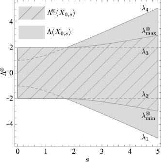
Figure 1: Numerical range and product numerical range for matrices $X_{0,s}$, which belong to the family (11).

First we analyze the edge. On the edge (one of the variables $p,q$ is 0 or 1) the square root vanishes, the remaining part is convex and thus the extreme points are $(p,q)\in\{(0,0),(0,1),(1,0),(1,1)\}$. Thus the maximum value on the edge is 2. If we assume that $p,q\notin\{0,1\}$, we have to find zeros of appropriate derivatives. The extremum value is $\sqrt{t^{4}+10t^{2}+9}/2t$ for $t\geq\sqrt{3}$. The lower estimate is obtained similarly. Thus the exact formula for the product numerical range reads:

$$\mathrm{\Lambda}^{\!\otimes}\!\left(X_{t,s}\right)=[-f(t+s),f(t+s)],$$ (16)

where

$$f(t)=\left\{\begin{array}[]{c c c}2&\text{ for }&t\in[0,\sqrt{3})\\ \sqrt{t^{4}+10t^{2}+9}/2t&\text{ for }&t\in[\sqrt{3},\infty)\end{array}\right..$$ (17)

Note that the product numerical range depends only on the sum of the parameters $s$ and $t$, whereas the numerical range depends on the values of both of them. The minimum and the maximum values in the numerical range and the product numerical range of the matrix $X_{t,s}$ are compared in Fig. 1.

Let us consider a more general family of matrices for $t,s\geq 0$

$$Y_{t,s}=\left(\begin{array}[]{cccc}a&0&0&t\\ 0&b&s&0\\ 0&s&c&0\\ t&0&0&d\end{array}\right).$$ (18)

For given $a,b,c,d$, one can obtain a similar result as above, but in general the formulas are very complex due to the higher number of parameters. However, it is easy to obtain the following bound

$$[f(s+t),g(s+t)]\subset\mathrm{\Lambda}^{\!\otimes}\!\left(Y_{s,t}\right),$$ (19)

where

$$f(t)=\min\{\min(a,b,c,d),\frac{1}{4}\mathrm{tr}Y_{0,0}-\frac{1}{2}t\},$$ (20)

and

$$g(t)=\max\{\max(a,b,c,d),\frac{1}{4}\mathrm{tr}Y_{0,0}+\frac{1}{2}t\}.$$ (21)

II.2.2 A tridiagonal Hermitian matrix

Consider another family of Hermitian matrices of size four, written in the standard product basis,

$$D=\left[\begin{array}[]{cccc}\frac{1}{2}&a&0&0\\ {a}^{*}&\frac{1}{2}&b&0\\ 0&{b}^{*}&\frac{1}{2}&c\\ 0&0&{c}^{*}&\frac{1}{2}\end{array}\right],$$ (22)

where $a$ and $b$ are arbitrary complex numbers and $c=xa$ for some arbitrary real number $x$.

This family was introduced in SZ09 as a useful example for studying block positivity. Here we deal with the product numerical range of $D$, but the two concepts are closely related, since a Hermitian matrix acting on a bipartite Hilbert space is block positive iff its product numerical range belongs to $\mathbb{R}_{+}$. Following the lines of SZ09 , with some additional effort, one obtains an explicit result

$$\mathrm{\Lambda}^{\!\otimes}\!\left(D\right)=\left[\frac{1}{2}-G,\frac{1}{2}+G\right],$$ (23)

where

$$G=\frac{1}{4}\left(|a+c|+\sqrt{|a-c|^{2}+|b|^{2}}\right).$$ (24)

II.2.3 Family of isospectral Hermitian operators

It is instructive to study product numerical range for a family of Hermitian operators with a fixed spectrum and varying eigenvectors. Any unitary $4\times 4$ matrix $U$ may be represented in a canonical form:

$$U=(V_{A}\otimes V_{B})\;U_{d}\;(W_{A}\otimes W_{B})\;,$$ (25)

where $V_{A},V_{B},W_{A},W_{B}\in U(2)$, while $U_{d}$ is a unitary matrix of size four expressed in the form KC2001

$$U_{d}(\alpha_{1},\alpha_{2},\alpha_{3})=\exp(i\sum_{k=1}^{3}\alpha_{k}\sigma_{k}\otimes\sigma_{k}).$$ (26)

Here $\sigma_{k}$ denotes the Pauli matrices, and the three real parameters $\alpha_{i}$ belong to the interval $\left[0,\frac{\pi}{4}\right]$.

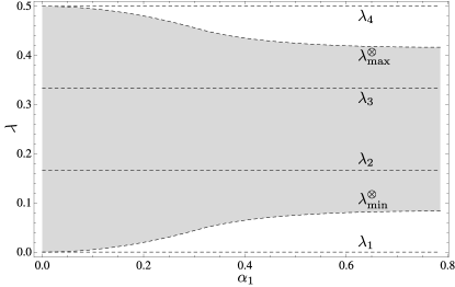
Figure 2: Product eigenvalues and product numerical range (gray region) of the one-parameter ($\alpha_{1}$) family of matrices given by Eq. (27) with eigenvalues $\lambda_{1}=0,\lambda_{2}=1/6,\lambda_{3}=1/3,\lambda_{4}=1/2$.

Consider a density matrix obtained from the diagonal matrix $E(x_{1},x_{2},x_{3})=\mathrm{diag}(x_{1},x_{2},x_{3},1-x_{1}-x_{2}-x_{3})$ by a non-local unitary rotation,

$$\rho(\alpha_{1},x_{i})=U_{d}EU_{d}^{\dagger},$$ (27)

with $\alpha_{2}=\alpha_{3}=0$. Figure 2 presents the dependence of its product numerical range as a function of the non-locality phase $\alpha_{1}$.

II.2.4 Random Hermitian matrices of order four

As shown in the above examples, the lower edge of the product numerical range of a Hermitian matrix $X$ of order four is interlaced between its two smallest eigenvalues, $\lambda_{\rm min}^{\otimes}\in[\lambda_{1},\lambda_{2}]$. We have already seen that these bounds can be saturated, so the exact position of $\lambda_{\rm min}^{\otimes}$ is $X$ dependent. However, following the statistical approach, one may pose the question how the edge is located with respect to both eigenvalues for a random Hermitian operator.

To analyze this problem we generated numerically a $5\times 10^{5}$ random Hermitian matrices according to the flat (Hilbert–Schmidt) measure in the set $\Omega$ of normalized density matrices of size $N=4$. The joint probability distribution for the eigenvalues reads SZ04

$$P(\lambda_{1},\lambda_{2},\lambda_{3},\lambda_{4})\ =\ \frac{15!}{3456}\;\delta\bigl{(}1-\sum_{j=1}^{4}\lambda_{j}\bigr{)}\prod_{i<j}^{4}(\lambda_{i}-\lambda_{j})^{2}.$$ (28)

By construction, the eigenvalues sum to unity, and this normalization sets the scale. It is possible to integrate out of the above formula any chosen three eigenvalues and obtain an explicit probability distribution for the last one. For instance the distribution for the smallest eigenvalue has the form

$$P(\lambda_{1})\ =\ 60(1-4\lambda_{1})^{14}\ \Theta(\lambda_{1})\;\Theta(1/4-\lambda_{1})\ ,$$ (29)

where $\Theta(x)$ is the Heaviside function.

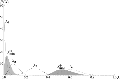
Figure 3: Probability density of eigenvalues $\lambda_{1},\lambda_{2},\lambda_{3},\lambda_{4}$ (dashed/dotted lines) and product values $\lambda_{\rm min}^{\otimes},\lambda_{\rm max}^{\otimes}$ (dark histograms) for a random two-qubit density matrix, generated according to the Hilbert-Schmidt measure (28).

Figure 3 presents the probability distributions for ordered eigenvalues, $\lambda_{1}\leq\lambda_{2}\leq\lambda_{3}\leq\lambda_{4}$, obtained analytically by integration of (28). These distributions are compared with the distributions $P(\lambda_{\rm min}^{\otimes})$ and $P(\lambda_{\rm max}^{\otimes})$ obtained numerically. As follows from (10) $\lambda_{\rm min}^{\otimes}$ is located between the two smallest eigenvalues, while $\lambda_{\rm max}^{\otimes}$ is interlaced by the two largest eigenvalues $\lambda_{3}$ and $\lambda_{4}$. Note that the histogram is not symmetric with respect to the change $\lambda_{1}\leftrightarrow\lambda_{4}$ and $\lambda_{\rm min}^{\otimes}\leftrightarrow\lambda_{\rm max}^{\otimes}$, since the eigenvalues are ordered, so the mean distance of the smallest eigenvalue to zero is smaller than the mean distance of the largest eigenvalue to unity.

II.3 Non–Hermitian case and Multipartite operators

The above analysis can be extended in a natural way for Hilbert spaces with $m$-fold tensor product structure, used to describe quantum systems consisting of $m$ subsystems,

$$\mathcal{H}_{N}\ =\ \mathcal{H}_{n_{1}}\otimes\cdots\otimes\mathcal{H}_{n_{m}},$$ (30)

with $N=n_{1}\dots n_{m}$. In the case of an operator $X$ acting on this space, its product numerical range consists of all expectation values $\langle\psi_{\rm prod}|X|\psi_{\rm prod}\rangle$ among pure product states, $|\psi_{\rm prod}\rangle=|\phi_{1}\rangle\otimes\dots\otimes|\phi_{m}\rangle$.

If the number $m$ of subsystems is larger than two, there exist operators for which product numerical range forms a set which is not simply connected thomas08significance ; PGMSCZ10 . In fact the genus of this set can be greater than one. To show an illustrative example, we consider a unitary matrix of size two

$$U=\left[\begin{array}[]{cc}1&0\\ 0&e^{i\phi}\end{array}\right].$$ (31)

The product numerical range of $U^{\otimes n}$ can be found analytically for any integer $n$ by applying an extension of the formula (8) to multipartite systems. Numerical range of $U$ forms an interval $I$ joining the complex eigenvalue $e^{i\phi}$ with the unity. Thus to find $\mathrm{\Lambda}^{\!\otimes}\!\left(U^{\otimes n}\right)$, it suffices to compute the $n$-fold Minkowski power of the interval $I$ on the complex plane. More explicitly, $\mathrm{\Lambda}^{\!\otimes}\!\left(U^{\otimes n}\right)$ consists of all the points $z_{1}z_{2}\ldots z_{n}$, where $z_{i}=1-\lambda_{i}+\lambda_{i}e^{i\phi}$ and $\lambda_{i}\in\left[0,1\right]$ for all $i\in\left\{1,2,\ldots,n\right\}$. Let us denote by $f\left(\alpha\right)$ the modulus $\left|z\right|$ of $z=1-\lambda+\lambda e^{i\phi}$ as a function of the phase $\alpha:=\textnormal{Arg}\left(z\right)$. Obviously, $f$ is a convex function of $\alpha$. One can relatively easy get an explicit expression for $f$,

$$f\left(\alpha\right)=\frac{\cos\left(\phi/2\right)}{\cos\left(\alpha-\phi/2\right)}.$$ (32)

Thus the numbers $z$ of the form $z=1-\lambda+\lambda e^{i\phi}$, $\lambda\in\left[0,1\right]$ have a parametrization $\alpha\mapsto e^{i\alpha}f\left(\alpha\right)$ with $\alpha\in\left[0,\phi\right]$ and $f$ given by formula (32). Because of the convexity of $f$, for a fixed $\textnormal{Arg}\left(z_{1}z_{2}\ldots z_{n}\right)$, the minimum of $\left|z_{1}z_{2}\ldots z_{n}\right|$ is attained when $z_{1}=z_{2}=\ldots=z_{n}$. The resulting curve marks the border of $\mathrm{\Lambda}^{\!\otimes}\!\left(U^{\otimes n}\right)$ and has a parametrization

$$\left[0,\phi\right]\ni\alpha\mapsto e^{in\alpha}\left(\frac{\cos\left({\phi/2}\right)}{\cos\left(\alpha-{\phi/2}\right)}\right)^{n}.$$ (33)

The remaining parts of the border of $\mathrm{\Lambda}^{\!\otimes}\!\left(U^{\otimes n}\right)$ are included in the $n$ segments $\left\{\left[e^{i\left(k-1\right)\phi},e^{ik\phi}\right]\right\}_{k=1}^{n}$. This follows because the maximum of $\left|z_{1}z_{2}\ldots z_{n}\right|$ for a fixed $\beta=\textnormal{Arg}\left(z_{1}z_{2}\ldots z_{n}\right)$ is attained for $z_{1}=z_{2}=\ldots=z_{k-1}=e^{i\phi}$, $z_{k}=e^{i\left(\beta-k\phi\right)}$ and $z_{k+1}=z_{k+2}=\ldots=z_{n}=1$, where $k=\lfloor\beta/\phi\rfloor$. In Figure 4 we choose $\phi=\frac{3\pi}{5}$ and plot the product numerical ranges of $U^{\otimes n}$ for $n=1,2,\ldots,8$.

  $n=1$

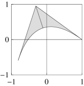
  $n=2$

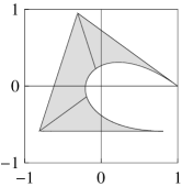
  $n=3$

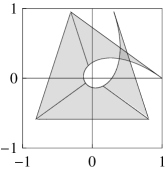
  $n=4$

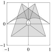
  $n=5$

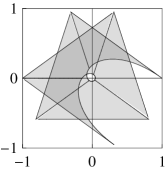
  $n=6$

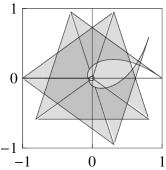
  $n=7$

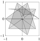
  $n=8$

Figure 4: Product numerical range of $U^{\otimes n}$ for $U$ specified in (31) with $\phi=3\pi/5$ and $n=1,\ldots,8$.

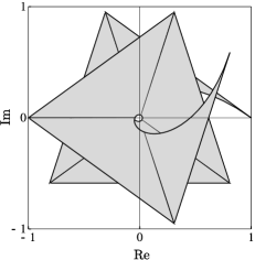
Figure 5: Product numerical range of $U^{\otimes 7}$ (plotted in gray) forms a set of genus $2$. The matrix $U$ is given by Eq. (31) with $\phi=3\pi/5$.

Observe that if $0$ does not belong to the numerical range of $U$, it does not belong to the product numerical range of $U^{\otimes n}$. Hence if for sufficiently large exponent $n$ the product range ’wraps around’ zero, the set $\mathrm{\Lambda}^{\!\otimes}\!\left(U^{\otimes n}\right)$ is not simply connected.

As one may notice in Figure 4, it is possible to construct a tensor product of operators such that its product numerical range has genus two. If we magnify picture number seven from Figure 4, it becomes evident that the genus of $\mathrm{\Lambda}^{\!\otimes}\!\left(U^{\otimes 7}\right)$ is equal to two (cf. Figure 5). Observe that if $n$ is further increased, the genus of $\mathrm{\Lambda}^{\!\otimes}\!\left(U^{\otimes n}\right)$ is not smaller than one, although the size of the hole around $z=0$ shrinks exponentially fast. More precisely, the distance between the set $\Lambda\left(U\right)$ and zero is $\cos\left(\phi/2\right)$, which implies that the distance between $\Lambda^{\otimes}\left(U^{\otimes n}\right)$ and zero equals $[\cos\left(\phi/2\right)]^{n}$ for arbitrary $n$.

In general, finding the product numerical range of a non-Hermitian operator without the tensor product structure is not a simple task. However, in the special case of a normal operator $X$, which can be diagonalized by product of unitary matrices, a useful parameterization of its product numerical range was described in PGMSCZ10 .

III Separable numerical range

Consider a tensor product Hilbert space $\mathcal{H}_{N}=\mathcal{H}_{K}\otimes\mathcal{H}_{M}$ and the set $\Omega$ of all normalized states acting on it, $\rho\in\Omega\Leftrightarrow\rho=\rho^{\dagger},\rho\geq 0,{\rm Tr}\rho=1$. One distinguishes its subset $\Omega_{\rm sep}$ of separable states, i.e. states that can be represented as a convex combination of product states,

$$\rho\in\Omega_{\rm sep}\ \Leftrightarrow\ \rho\in\Omega{\rm\quad and\quad}\rho=\sum_{i}p_{i}\;\rho_{i}^{(K)}\otimes\rho_{i}^{(M)}$$ (34)

Here positive coefficients $p_{i}$ form a probability vector, while $\rho_{i}^{(K)}$ and $\rho_{i}^{(M)}$ denote arbitrary states acting on $\mathcal{H}_{K}$ and $\mathcal{H}_{M}$, respectively. Any state $\rho$ which cannot be represented in the above form is called entangled BZ06 . Hence this definition depends on the particular choice of the tensor product structure, $\mathcal{H}_{N}=\mathcal{H}_{K}\otimes\mathcal{H}_{M}$.

Observe that Definition 6 of the product numerical range of an operator $X$ acting on $\mathcal{H}_{K}\otimes\mathcal{H}_{M}$ can be formulated as

$$\mathrm{\Lambda}^{\!\otimes}\!\left(X\right)=\left\{{\rm Tr}X\rho:\rho=|\psi_{A}\rangle\otimes|\psi_{B}\rangle\langle\psi_{A}|\otimes\langle\psi_{B}|\right\}.$$ (35)

It is then natural to introduce an analogous definition of separable numerical range

$$\Lambda^{\rm sep}(X):=\left\{{\rm Tr}X\rho:\rho\in\Omega_{\rm sep}\right\}.$$ (36)

Since any product state is separable, the product numerical range forms a subset of the separable numerical range, $\mathrm{\Lambda}^{\!\otimes}\!\left(X\right)\subset\Lambda^{\rm sep}(X)$. By definition, the set $\Omega_{\rm sep}$ of separable states is convex. This fact allows us to establish a simple relation between both sets.

Proposition 1

Separable numerical range forms the convex hull of the product numerical range,

$$\Lambda^{\rm sep}(X)={\rm co}(\mathrm{\Lambda}^{\!\otimes}\!\left(X\right))$$

Proof. Assume that $\lambda\in{\rm co}(\mathrm{\Lambda}^{\!\otimes}\!\left(X\right))$, so it can be represented as a convex combination of points belonging to the product numerical range, $\lambda=\sum_{i}p_{i}\lambda_{i}$. Taking the convex combination of the corresponding product states $|\phi_{i}\rangle=|\psi_{i}^{A}\rangle\otimes|\psi_{i}^{B}\rangle$ we get a separable mixed state $\rho=\sum_{i}p_{i}|\phi_{i}\rangle\langle\phi_{i}|$ such that ${\rm Tr}X\rho=\lambda$. A similar reasoning shows that if $\lambda\notin{\rm co}(\mathrm{\Lambda}^{\!\otimes}\!\left(X\right))$ there is no separable state $\rho$ such that ${\rm Tr}X\rho=\lambda$. $\blacksquare$

Following PGMSCZ10 one can note that if $A$ or $B$ is normal then $\Lambda^{\rm sep}(A\otimes B)=\Lambda(A\otimes B)$.

Since product numerical range of a Hermitian operator forms an interval, in this case the separable and product numerical ranges do coincide. This is not the case in general. A typical example is shown in Figs. 6b and 6c, in which the separable numerical range forms a proper subset of the standard numerical range and includes the product numerical range as its proper subset.

Consider, for instance a unitary matrix $U$ of size $4$ with a non-degenerate spectrum. Its numerical range is then formed by a quadrangle inscribed into the unit circle. If all eigenvectors of this matrix are entangled, the product numerical range of $U$ does not contain any of its eigenvalues. In a generic case $\mathrm{\Lambda}^{\!\otimes}\!\left(U\right)$ is not convex and it forms a proper subset of $\Lambda^{\rm sep}(U)$ – see Fig. 6.

\begin{overpic}[width=130.08731pt]{separable0} \put(80.0,12.0){\scriptsize$\alpha=0$} \end{overpic} \begin{overpic}[width=130.08731pt]{separable2} \put(80.0,12.0){\scriptsize$\alpha=\frac{\pi}{8}$} \end{overpic}

\begin{overpic}[width=130.08731pt]{separable3} \put(80.0,12.0){\scriptsize$\alpha=\frac{3\pi}{16}$} \end{overpic} \begin{overpic}[width=130.08731pt]{separable4} \put(80.0,12.0){\scriptsize$\alpha=\frac{\pi}{4}$} \end{overpic}

Figure 6: Numerical range (light gray), separable numerical range (dark gray) and product numerical range (black dots obtained by random sampling) of family of matrices $X_{\alpha}=U_{d}(\alpha,0,0)\cdot\mathrm{diag}(i,-1,-i,1)\cdot U_{d}(\alpha,0,0)^{\dagger}$, where $U_{\alpha}$ is given by Eq. (26) for $\alpha=0,\pi/8,3\pi/16,\pi/4$. In the case of $\alpha=0$ the eigenvectors of $X$ form orthonormal canonical basis and $X$ is normal therefore $\Lambda^{\rm sep}(X)=\Lambda(X)$. In the case of $\alpha=\pi/4$ all eigenvectors of $X$ are maximally entangled states and $\Lambda^{\rm sep}(X)=\mathrm{\Lambda}^{\!\otimes}\!\left(X\right)$.

III.1 $k$–Entangled numerical range

Any pure state in a $N=KM$ dimensional bipartite Hilbert space can be represented by its Schmidt decomposition,

$$|\psi\rangle=\sum_{i=1}^{K}\sum_{j=1}^{M}A_{ij}|i\rangle\otimes|j\rangle=\sum_{i=1}^{K}\sqrt{\mu_{i}}\;|i^{\prime}\rangle\otimes|i^{\prime\prime}\rangle.$$ (37)

We the have assumed here that $K\leq M$ and denoted a suitably rotated product basis by $|i^{\prime}\rangle\otimes|i^{\prime\prime}\rangle$. The eigenvalues $\mu_{i}$ of a positive matrix $AA^{\dagger}$ are called the Schmidt coefficients of the bipartite state $|\psi\rangle$. The normalization condition $|\psi|^{2}=\langle\psi|\psi\rangle=1$ implies that $||A||^{2}_{\rm HS}=\mathrm{tr}AA^{\dagger}=1$, so the Schmidt coefficients $\mu_{i}$ form a probability vector – see e.g. BZ06 .

The state $|\psi\rangle$ is separable iff the $K\times M$ matrix of coefficients $A$ is of rank one, so the corresponding vector of the Schmidt coefficients is pure. A given mixed state $\rho$ is called separable if it can be represented as a convex combination of product pure states. This notion can be generalized in a natural way, and in the theory of quantum information TH00 once considers set $\Omega^{({\rm k})}$ of states which can be decomposed into a convex combination of states with the Schmidt number not larger than $k$. In symbols, $\rho=\sum_{j=1}p_{j}|\phi_{j}\rangle\langle\phi_{j}|,$ with all vectors $|\phi_{j}\rangle=\sum_{i=1}^{k}\xi_{i}|\psi^{A}_{i}\rangle\otimes|\psi^{B}_{i}\rangle$ of Schmidt rank at most $k$. We may choose $k$ to be $1,\dots,K$, where $K=M$ denotes the dimensionality of each subsystem. By definition, $\Omega^{(1)}=\Omega_{\rm sep}$ represents the set of separable states, while $\Omega^{({\rm K})}=\Omega$ denotes the entire set of mixed quantum states.

Making use of the definition of the subset $\Omega^{({\rm k})}$ of the set of all states in (3) one obtains an entire hierarchy of restricted numerical ranges denoted by $\Lambda^{(k)}$. As the elements of $\Omega^{({\rm k})}$ are called $k$-entangled states SSZ09 , the set $\Lambda^{({\rm k})}(X)$ will be referred to as numerical range restricted to $k$–entangled states.

For $k=1$ one has $\Omega^{(1)}=\Omega_{\rm sep}$ so in this case one obtains the separable numerical range, $\Lambda^{(1)}=\Lambda^{\rm sep}$. Note that in this convention a $1$-entangled state means a separable state. In the other limiting case $k=K$, $\Omega_{K}=\Omega$ and one arrives at the standard numerical range, $\Lambda^{(K)}=\Lambda$. The following chain of inclusions $\Lambda^{\otimes}\subset\Lambda^{(1)}\subset\Lambda^{(2)}\subset\cdots\subset\Lambda^{({\rm K})}=\Lambda$ holds by construction. This implies inequalities between the corresponding restricted numerical radii, $r^{\otimes}\leq r^{(1)}\leq r^{(2)}\leq\dots,\leq r^{(K)}=r$.

IV Applications in quantum information theory

In this section we link various problems in the theory of quantum information processing which have one thing in common: they can be analyzed using the restricted numerical range or related notions.

IV.1 Block positive matrices and entanglement witnesses

Let us start by recalling the standard definition of block-positivity BZ06 . A Hermitian matrix $X$ acting on the tensor product Hilbert space, ${\cal H}_{N}={\cal H}_{M}\otimes{\cal H}_{K}$, is called block positive, if it is positive on all product states. Making use of the notation introduced in Sec. II this property reads, $\lambda_{\rm min}^{\otimes}(X)\geq 0$. Therefore checking if a given Hermitian matrix is block-positive is equivalent to showing that its product numerical range forms a subset of $[0,\infty)$.

Block positive matrices arise in a characterization of positive quantum maps by the theorem of Jamiołkowski Ja72 . A map $\Phi$ taking operators on $\mathcal{H}_{K}$ to operators on $\mathcal{H}_{M}$, is called positive, if it maps positive operators to positive operators. Let $|\Psi_{+}\rangle\langle\Psi_{+}|$ denote the orthogonal projection onto the maximally entangled state $|\Psi_{+}\rangle=\frac{1}{\sqrt{K}}\sum_{i=1}^{K}|i\rangle|i\rangle$ acting on $\mathcal{H}_{K}\otimes\mathcal{H}_{K}$. The Jamiołkowski theorem states that $\Phi$ is positive iff the corresponding dynamical matrix (Choi matrix Cho75a ), $D_{\Phi}=\left(\Phi\otimes\mathbbm{1}\right)|\Psi_{+}\rangle\langle\Psi_{+}|$, is block positive. This leads us to the following characterization of positive maps in terms of the product numerical range of $D_{\Phi}$,

Proposition 2

Let $\Phi$ be a linear map taking operators on $\mathcal{H}_{K}$ to operators on $\mathcal{H}_{M}$. Then

$$\Phi\textrm{ is positive }\Leftrightarrow\ \mathrm{\Lambda}^{\!\otimes}\!\left(D_{\Phi}\right)\subset[0,\infty).$$ (38)

That is, the product numerical range of $D_{\Phi}$ has to be contained in the positive semiaxis in order for $\Phi$ to be positive. As discussed in Section III, for any Hermitian $D$, its product and separable numerical ranges do coincide. Consequently, positivity of $\Phi$ can be formulated with $\Lambda^{\rm sep}(D_{\Phi})$. The positivity condition reads: ${\rm Tr}D_{\Phi}\rho\geq 0$ for any separable $\rho$. This is the same as $\Lambda^{\rm sep}\left(D_{\Phi}\right)\subset\left[0;+\infty\right)$.

We recall that a map $\Phi$ is called $k$-positive if $\Phi\otimes\mathbbm{1}_{k}$ is a positive map. If this is the case for arbitrary $k\in\mathbbm{N}$ the map is called completely positive. The famous theorem by Choi Cho75a concerning completely positive maps can be expressed in a similar manner,

Proposition 3

Let $\Phi$ be a linear map taking operators on $\mathcal{H}_{K}$ to operators on $\mathcal{H}_{M}$. Then

$$\Phi\textrm{ is completely positive }\Leftrightarrow\ \mathrm{\Lambda}\left(D_{\Phi}\right)\subset[0,\infty).$$ (39)

The difference is that (38) refers to the product numerical range of $D_{\Phi}$ whereas (39) concerns the standard numerical range. Note that $\mathrm{\Lambda}\left(D_{\Phi}\right)\subset[0,\infty)$ is just another way of writing that $D_{\Phi}$ is a positive operator.

Positive maps find a direct application in the theory of quantum information due to a theorem by the Horodecki family HHH96a : a state $\sigma$ of a bipartite system is separable iff $(\Phi\otimes{\mathbbm{1}})\sigma\geq 0$ for any positive map $\Phi$. In the opposite case, the state $\sigma$ is entangled.

The above results explain recent interest in characterization of the set of positive maps. A block positive matrix $W:=D_{\Phi}$ which corresponds to a map which is positive but not completely positive, is called an entanglement witness, since it can be used to detect quantum entanglement. As discussed in sec. III, product and separable numerical ranges coincide for Hermitian operators. Thus the set of entanglement witnesses consists of Hermitian operators $W$ such that ${\rm Tr}W\rho\geq 0$ for all separable $\rho$ and there exists an entangled state $\sigma$ such that ${\rm Tr}W\sigma<0$. The set of separable quantum states can thus be characterized by a suitably chosen set of entanglement witnesses. Such an approach was advocated in a recent work by Sperling and Vogel SV09 , in which various methods for obtaining the minimal product value $\lambda_{\rm min}^{\otimes}$ of Hermitian matrices were analyzed.

Bound 9 implies that the spectrum of an entanglement witness for any state of a $K\times K$ system has at most $(K-1)^{2}$ negative eigenvalues, in accordance with recent results of Sarbicki Sa08 . In the simplest case of $K=2$, one recovers the known statement that any non-trivial entanglement witness in the two-qubit system has exactly one negative eigenvalue STV98 .

Our study of product numerical range of a Hermitian operator can thus be directly applied to the positivity problem. For instance, consider the family of one-qubit maps described by the dynamical matrix $D=D(a,b,c)$ defined in (22). It is clear that these matrices are block positive iff $G\leq 1/2$. Therefore the expression (24) for $G=G(a,b,c)$ gives us explicit constraints under which the map corresponding to $D(a,b,c)$ is positive. If this map is not completely positive, the matrix $D$ can be used as a witness of quantum entanglement.

In the above case corresponding to maps acting on $2$ dimensional Hilbert space ${\cal H}_{2}$ any $2$–positive map is completely positive. This is a consequence of the theorem of Choi Cho75a , which implies that if a map acting on $K$ dimensional Hilbert space is $K$ positive, it is also completely positive. Thus for maps acting on a $K$–dimensional system, it is interesting to study $k$–positivity for $k=1$ (equivalent to positivity), $k=2,\dots K-1$ and $k=K$ (complete positivity). In general $k$-block positive matrices are related to $k$–positive maps. We are thus in a position to formulate the generalized Jamiołkowski–Choi theorem Ra07 ; SSZ09 making use of the concept of the restricted numerical range.

Proposition 4

Let $\Phi$ be a linear map taking operators on $\mathcal{H}_{K}$ to operators on $\mathcal{H}_{M}$. Then

$$\Phi\textrm{ is $k$--positive }\Leftrightarrow\ \Lambda^{(k)}\left(D_{\Phi}\right)\subset[0,\infty).$$ (40)

As we explain in the next section, a special case of Proposition 4 for $k=2$ is of relevance to the distillability problem for quantum states.

IV.2 $n$–copy distilability of a quantum state

It has been known for a long time diVicenzo00 that bi-partite states with distillable entanglement are closely related to $2$-positive maps and hence to $2$-block positive operators (cf. also Cl05 ; SSZ09 ). The precise relation between distillability and $2$-block positivity is the following. Let $\rho$ be an arbitrary state on a bipartite space $\mathcal{H}_{N}=\mathcal{H}_{K}\otimes\mathcal{H}_{M}$. Assume that we allow only LOCC operations on a single copy of $\rho$. The state can be distilled into a maximally entangled state only if the partial transpose $\left({\rm 1l}\otimes T\right)\rho$ is not a $2$-block positive operator, i.e. it is not positive on states with Schmidt rank $2$. Otherwise, $\rho$ is one-copy undistillable. Writing this in terms of $k$-entangled numerical ranges (cf. Section III.1), we get the following proposition.

Proposition 5

A state with a density matrix $\rho$ on a bi-partite space $\mathcal{H}_{N}=\mathcal{H}_{K}\otimes\mathcal{H}_{M}$ is one-copy undistillable if and only if the $2$-entangled numerical range of its partial transpose is contained in the nonnegative semiaxis, $\Lambda^{\left(2\right)}\left(\left({\rm 1l}\otimes T\right)\rho\right)\in\left[0;+\infty\right)$.

If a state $\rho$ turns out to be one-copy undistillable, it is still possible that a number of copies of $\rho$ can be used for entanglement distillation. Proposition 5 is easily generalized to that situation.

Proposition 6

Let $\rho$ correspond to a state on a bi-partite space $\mathcal{H}_{N}=\mathcal{H}_{K}\otimes\mathcal{H}_{M}$. For any integer $n$, the state is $n$-copy undistillable if and only if the $2$-entangled numerical range of $\left({\rm 1l}\otimes T\right)\rho^{\otimes n}$ is contained in the nonnegative semiaxis, $\Lambda^{\left(2\right)}\left(\left({\rm 1l}\otimes T\right)\rho^{\otimes n}\right)\in\left[0;+\infty\right)$.

The symbol $\Lambda^{\left(2\right)}$ in Proposition 6 refers to positivity on states of Schmidt rank $2$, where the Schmidt rank is calculated w.r.t. the splitting $\mathcal{H}_{N}^{\otimes n}=\mathcal{H}^{\otimes n}_{K}\otimes\mathcal{H}^{\otimes n}_{M}$ of the multipartite space. This is important to notice because many different splittings of $\mathcal{H}_{N}^{\otimes n}$ into a tensor product of two factors are possible. Evidently, Proposition 6 is nothing but Proposition 5 applied to $\rho^{\otimes n}$ in place of $\rho$. This is easy to understand because the tensor product $\rho^{\otimes n}$ represents a number $n$ of identical, independent copies of the state $\rho$, e.g. coming from a source that produces $\rho$.

It is natural to mention here a fundamental question concerning distillability of quantum states. Using the language of numerical ranges, we can formulate the problem in the following way: Given a density matrix $\rho$ on a bi-partite Hilbert space $\mathcal{H}_{N}^{\otimes n}=\mathcal{H}^{\otimes n}_{K}\otimes\mathcal{H}^{\otimes n}_{M}$ s.t. $\Lambda\left(\left({\rm 1l}\otimes T\right)\rho\right)\not\in\left[0;+\infty\right)$, can we infer that $\Lambda^{\left(2\right)}\left(\left({\rm 1l}\otimes T\right)\rho^{\otimes n}\right)\not\in\left[0;+\infty\right)$ for some positive integer $n$? In other words, is a bi-partite state $\rho$ with a negative partial transpose always distillable, possibly using a huge number $n$ of copies of $\rho$? This question has not yet been answered, despite a considerable effort and some partial results (cf. e.g. Pankowski ).

IV.3 Minimum output entropy and product numerical range

Consider a completely positive map $\Phi$ acting on the set $\Omega_{N}$ of normalized quantum states of dimension $N$. Minimum output entropy (see e.g. (petz, , Chapter 7)) is defined as

$$S_{\min}\left(\Phi\right)=\min_{\rho}\left\{S\left(\Phi(\rho)\right)\right\},$$ (41)

with $\rho\in\Omega_{N}$. Since the von Neumann entropy is concave, the minimum is attained on the boundary and thus

$$S_{\min}\left(\Phi\right)=\min_{|\psi\rangle\langle\psi|}\left\{S\left(\Phi(|\psi\rangle\langle\psi|)\right)\right\},$$ (42)

where $|\psi\rangle\langle\psi|\in\Omega_{N}$ are pure states. Therefore the minimum output entropy can be interpreted as a certain measure of decoherence introduced by the channel.

In king01minimal ; king02additivity it was proven that minimum output entropy (and thus Holevo capacity) is additive for unital channels. It is now known however that minimum output entropy is not additive in the general case hastings09counterexample . Here we provide a characterization of the minimum output entropy for one-qubit channels using product numerical range of the dynamical matrix.

Proposition 7

Let $\Phi$ be a CP-TP map acting on $\Omega_{2}$. Then

$$S_{\min}\left(\Phi\right)=\lambda\log(\lambda)+(1-\lambda)\log(1-\lambda),$$ (43)

where $\lambda$ is a minimal value of product numerical range for the dynamical matrix $D_{\Phi}$

$$\lambda=\lambda^{\otimes}_{\min}(D_{\Phi}).$$ (44)

Proof. Let us define $f(x)=-x\log_{2}(x)-(1-x)\log_{2}(1-x)$, which is increasing for $x\in[0,\frac{1}{2}]$.

Directly from the definition of minimum output entropy we can write

$$S_{\min}\left(\Phi\right)=\min_{|i\rangle}S(\Phi(|i\rangle\langle i|))=\min_{|i\rangle}f(\lambda_{\min}(\Phi(|i\rangle\langle i|)))=f\left(\min_{|i\rangle}\lambda_{\min}(\Phi(|i\rangle\langle i|))\right).$$ (45)

Now since $\langle k|\Phi(|i\rangle\langle j|)|l\rangle=\langle k\otimes i|D_{\Phi}|l\otimes j\rangle$ (see (BZ06, , Eqn. 11.25)) we can rewrite the above expression as

$$S_{\min}\left(\Phi\right)=f\left(\min_{|i\rangle,|j\rangle}\langle j|\Phi(|i\rangle\langle i|)|j\rangle\right)=f\left(\min_{|i\rangle,|j\rangle}\langle j\otimes i|D_{\Phi}|j\otimes i\rangle\right)=f\left(\lambda^{\otimes}_{\min}(D_{\Phi})\right).$$ (46)

$\blacksquare$

Using the above proposition, we can easily calculate minimal output entropy for channels listed below.

First we consider the amplitude damping, phase damping, phase flip, bit-flip and and bit-phase flip channels. In all those cases we can see from the Kraus form that the spectrum of the dynamical matrix has two zero eigenvalues. Then the plane spanned by the two eigenvectors corresponding to the zero eigenvalue contains at least one product state CMW08 . Thus $\lambda_{\min}^{\otimes}(D_{\Phi})=0$ and the minimum output entropy for this channels is equal to zero. Using Proposition 7 one can also easily calculate minimum output entropy for some other one qubit channels. Consider the Werner-Holevo channel, described by the following dynamical matrix,

$$D_{\Phi_{\mathrm{HW}}}=\left(\begin{array}[]{cccc}\frac{p+1}{2}&0&0&0\\ 0&\frac{1-p}{2}&p&0\\ 0&p&\frac{1-p}{2}&0\\ 0&0&0&\frac{p+1}{2}\end{array}\right),$$ (47)

for $p\in[-1,1/3]$. In this case $\lambda_{\min}^{\rm loc}(D_{\Phi_{\mathrm{HW}}})=\frac{1}{2}(1-|p|)$ and thus

$$S_{\min}\left(\Phi_{\mathrm{HW}}\right) = -\frac{1}{2}(1-|p|)\log_{2}\frac{1}{2}(1-|p|)-\frac{1}{2}(1+|p|)\log_{2}\frac{1}{2}(1+|p|)$$ (48)

$$= -\frac{\log\left(\frac{1}{4}-\frac{p^{2}}{4}\right)+2p\tanh^{-1}(p)}{\log(4)}.$$ (49)

In the case of higher dimensional quantum channels we can use properties of product numerical range to check, whether for a given channel its minimal output entropy is equal zero.

Proposition 8

For any completely positive, trace preserving (CP-TP) map we have

$$S_{\min}\left(\Phi\right)=0\quad\text{ iff }\quad 1\in\Lambda^{\otimes}(D_{\Phi}).$$ (50)

Proof. Since $1\in\Lambda^{\otimes}(D_{\Phi})$, there exists $|i\rangle,|j\rangle$ such that

$$1=\langle i\otimes j|D_{\Phi}|i\otimes j\rangle=\langle i|\Phi(|j\rangle\langle j|)|i\rangle.$$ (51)

Because $\Phi$ is CP-TP channel, we have $\mathrm{tr}\Phi(|j\rangle\langle j|)=1$ and thus

$$\Phi(|j\rangle\langle j|)=|i\rangle\langle i|.$$ (52)

The proposition follows. $\blacksquare$

IV.4 Local discrimination of unitary operators

The problem of local distinguishability of multipartite quantum states was analyzed by Walgate et al. WSHV00 . Following their work, Duan et al. have shown DFY08 that two unitary operations $U_{1}$ and $U_{2}$ are locally distinguishable iff $0\in\mathrm{\Lambda}^{\!\otimes}\!\left(V\right)$ where $V=U_{1}^{\dagger}U_{2}$. If this is the case, then there exists a product state $|\psi\rangle=|\phi_{A},\phi_{B}\rangle$ such that the states $U_{1}|\psi\rangle$ and $U_{2}|\psi\rangle$ are orthogonal and thus distinguishable.

Our results on product numerical range allow us to solve the problem of local distinguishability for a wide class of unitary operators. If the operator $V=U_{1}^{\dagger}U_{2}$ has the tensor product structure, $V=V_{1}\otimes V_{2}$, the two unitaries $U_{1},U_{2}$ are distinguishable iff the numerical range of any of the factors $V_{1},V_{2}$ contains zero. This is the case when $0$ belongs to the convex hull of the spectrum of the factor $V_{1}$ or of the factor $V_{2}$.

Figure 7: a) Product numerical range for the matrix (53) with $\phi=2\pi/3$ and $\psi=10\pi/7$, b) The region in the space of parameters $\left(\phi,\psi\right)$ corresponding to locally distinguishable pairs $\left(U_{1},U_{2}\right)$ when $U_{1}^{\dagger}U_{2}=V\left(\phi,\psi\right)$.

Let us now deal with a more general case of $V$ without the tensor product structure. Consider for instance a family of unitary matrices of order four,

$$V\left(\phi,\psi\right)=\left[\begin{array}[]{cccc}1&0&0&0\\ 0&e^{i\phi}&0&0\\ 0&0&e^{i\psi}&0\\ 0&0&0&1\end{array}\right],$$ (53)

for $\phi,\psi\in\left[0,2\pi\right]$.

It is easy to show that the product numerical range of $V$ is a bounded region of $\mathbbm{C}$ whose border consists of the segments $\left[e^{i\phi},1\right]$, $\left[1,e^{i\psi}\right]$ and the line

$$\gamma:\left[0,1\right]\ni t\ \mapsto\ t^{2}e^{i\phi}+\left(1-t\right)^{2}e^{i\psi}+2t\left(1-t\right)\in\mathbbm{C}\ .$$ (54)

For example, Fig. 7a shows the shape of the product numerical range of $V(\frac{2\pi}{3},\frac{10\pi}{7})$.

Using Eq. (54), it is not difficult to check for which values of the phases $\phi$ and $\psi$ the product numerical range of $V\left(\phi,\psi\right)$ contains $0$, so any $U_{1}$ and $U_{2}$ such that $U_{1}^{\dagger}U_{2}=V\left(\phi,\psi\right)$ are locally distinguishable. Figure 7b) shows, in grey, the set of parameters $\left(\phi,\psi\right)$ corresponding to such distinguishable pairs $\left(U_{1},U_{2}\right)$. Explicitly, we have

$$0\in\mathrm{\Lambda}^{\otimes}\left(V\left(\phi,\psi\right)\right)\Leftrightarrow\Big{\{}|\sin\psi|\cos\phi+|\sin\phi|\cos\psi+2\sqrt{|\sin\phi\sin\psi|}\leqslant 0\\ \land\sin\phi\sin\psi\leqslant 0\land\left(\phi,\psi\right)\not\in\left\{\left(0,0\right),\left(2\pi,2\pi\right)\right\}\Big{\}}.$$ (55)

For any two unitary matrices $U_{1}$ and $U_{2}$ such that $V=U_{1}^{\dagger}U_{2}$ satisfies the above constraints, it is possible to find a product state $|\chi,\xi\rangle$ with the property $\langle\chi,\xi|V|\chi,\xi\rangle=0$. A detailed construction of this state, presented in Appendix A, allows one to design the scheme of local discrimination between the unitary gates $U_{1}$ and $U_{2}$.

IV.5 Local fidelity and entanglement measures

Several tasks of quantum information processing relay on the ability to approximate a given quantum state $\varrho_{1}$ by some other state $\varrho_{2}$. Alternatively, one attempts to distinguish $\varrho_{1}$ from $\varrho_{2}$. To characterize both problems quantitatively one may use fidelity, which can be interpreted as a ‘transition probability’ in the space of quantum states Uh76 ,

$$F(\varrho_{1},\varrho_{2})=[{\rm Tr}|\sqrt{\varrho_{1}}\sqrt{\varrho_{2}}|)]^{2}.$$ (56)

We are going to follow here the original definition by Jozsa Jo94 , but one has to be warned that some later articles use the name ‘fidelity’ for $\sqrt{F}$. If one of the states is pure, $\varrho_{1}=|\psi_{1}\rangle\langle\psi_{1}|$, formula (56) simplifies and $F=\langle\psi_{1}|\varrho_{2}|\psi_{1}\rangle$. Thus in this case fidelity has a simple interpretation of probability that the state $\varrho_{2}$ is projected onto a pure state $|\psi_{1}\rangle$.

Consider two arbitrary mixed states $\varrho_{1}$ and $\varrho_{2}$ acting on a Hilbert space ${\cal H}_{N}$. Although fidelity between these states is fixed and given by (56), one may pose a question to what extent fidelity can grow if local unitary operations are allowed. In other words, one asks about the fidelity between $\varrho_{1}$ and $U\varrho_{2}U^{\dagger}$ maximized over all unitaries $U\in U(N)$. This problem was studied in MMPZ08 , where the following bounds were established

$$F(p^{\uparrow},q^{\downarrow})\leq F(\varrho_{1},U\varrho_{2}U^{\dagger})\leq F(p^{\uparrow},q^{\uparrow})=F(p^{\downarrow},q^{\downarrow}).$$ (57)

The vectors $p$ and $q$ represent the spectra of $\varrho_{1}$ and $\varrho_{2}$, while the up/down arrows indicate that the eigenvalues are put in the non-decreasing (non-increasing, resp.) order. Arguments of the fidelity in the above equation denote thus diagonal matrices which represent classical states.

In this section we analyze an analogous problem for multipartite systems: What maximum fidelity between two given states of such a system can be achieved, if arbitrary local unitary operations are allowed? We provide a solution of this problem in the special case when both quantum states are pure and derive bounds for the local fidelity in the case where $\rho$ is a diagonal mixed state.

Let $|\phi\rangle$ be a vector and $\varrho$ an arbitrary mixed state, both on ${\cal H}_{AB}={\cal H}_{A}\otimes{\cal H}_{B}$. For simplicity we will restrict our attention to the symmetric case and assume that ${\rm dim}({\cal H}_{A})={\rm dim}({\cal H}_{B})=N$.

The fidelity of a mixed state with respect to a pure state is given by an expectation value, $F=\langle\phi|\varrho|\phi\rangle$. We are going to study the question to what extend this quantity can be increased by applying arbitrary local unitary operations $U_{A}\otimes U_{B}$. In other words, we look for the local fidelity defined as the maximum

$$F^{\rm max}(\varrho,\phi)=\max_{U_{A}\otimes U_{B}}\langle\phi|(U_{A}\otimes U_{B})^{\dagger}\varrho(U_{A}\otimes U_{B})|\phi\rangle.$$ (58)

It is instructive to relate this quantity to a generalized numerical radius of an operator $X$, defined as the largest modulus of an element of its numerical range. Similarly for an operator $X$ acting on a composed Hilbert space one defines product numerical radius as the largest modulus of an element of $\mathrm{\Lambda}^{\!\otimes}\!\left(X\right)$. This notion can be further generalized, and for any operator $X$ and an auxiliary operator $C$ acting on the Hilbert space $\mathcal{H}_{N}=\mathcal{H}_{K}\otimes\mathcal{H}_{M}$, one defines the $C$–product numerical radius thomas08significance ,

$$r_{C}^{\otimes}(X)=\max\{|z|:z=\mathrm{tr}(U_{1}\otimes U_{2})X(U_{1}\otimes U_{2})^{\dagger}C,\quad U_{1}\in U(K),\quad U_{2}\in U(M)\},$$ (59)

and other notions listed in Tab. 2. The problem of finding the local fidelity is then equivalent to determining the $C$–product numerical radius of the operator $X=|\phi\rangle\langle\phi|$ for $C=\varrho$.

Let us first solve the problem in the special case where the analyzed state is pure, $\varrho=|\psi\rangle\langle\psi|$. It is then useful to represent both pure states using their Schmidt decompositions (37),

$$|\phi\rangle=\sum_{i=1}^{N}\sqrt{\lambda_{i}}|i\rangle\otimes|i\rangle,{\quad}|\psi\rangle=\sum_{j=1}^{N}\sqrt{\mu_{j}}|j\rangle\otimes|j\rangle.$$ (60)

The vector $\lambda$ of Schmidt coefficients set in a decreasing (increasing) order will be denoted by $\lambda^{\downarrow}$ and $\lambda^{\uparrow}$, respectively. This notation allows one to formulate the following lemma.

Lemma 1

For arbitrary local unitary operation $U_{A}\otimes U_{B}$ and pure states $|\phi\rangle$, $|\psi\rangle$, one has

$$0\leq|\langle\psi|U_{A}\otimes U_{B}|\phi\rangle|^{2}\leq F(\mu^{\downarrow},\lambda^{\downarrow})=\left(\sum_{j=1}^{N}\sqrt{\lambda_{j}^{\downarrow}\mu_{j}^{\downarrow}}\right)^{2}.$$ (61)

The lower bound is a trivial consequence of the definition of fidelity. The upper bound follows from the theorem of Uhlmann which states that fidelity is given by the maximal overlap between purifications of both states, and the bound in (MMPZ08, , Eq. (4.19)). This result follows also from the recent work of Schulte-Herbrüggen et al. (SHGDH08, , Prop. IV.1).

If one of the states is separable, $|\phi\rangle=|\phi_{A}\rangle\otimes|\phi_{B}\rangle$, its Schmidt vector has only a single non-vanishing component, $\lambda^{\downarrow}=(1,0,\dots,0)$, so the overlap (61) is bounded by the largest Schmidt coefficient $\mu_{\rm max}$ of the state $|\psi\rangle$. This is a special case of the geometric measure of entanglement of a multipartite state $|\psi\rangle$, defined as the logarithm of the maximum projection on any product state WG03 ,

$$E_{g}(|\psi\rangle)\ =-{\rm log}\Bigl{(}\max_{U_{\rm loc}}|\langle\psi|U_{1}\otimes U_{2}\otimes\cdots\otimes U_{m}|0,\dots 0\rangle|^{2}\Bigr{)}\ .$$ (62)

Here $|0,\dots 0\rangle$ represents an arbitrary product state, so transforming it by a local unitary matrix one explores the entire set of separable pure states of the $m$–partite system. Observe that the argument of the logarithm in the above expression is just equal to the product numerical radius of the projector onto the analyzed state, $X=|\psi\rangle\langle\psi|$.

In recent papers HMMOV09 ; WS09 it was shown that the above maximization procedure becomes simpler if the multipartite state $|\psi\rangle$ is symmetric with respect to permutations of the subsystems, and all its coefficients in the product basis are non-negative. Then the maximum in (62) is achieved for the tensor product of a single unitary matrix, $U_{\rm loc}=U^{\otimes m}$, so the search for $E_{g}(\psi)$ can be reduced to the space of a smaller dimension. It is then natural to ask whether this observation can be generalized for the problem of determining the product numerical radius of any multipartite Hermitian operator $X$, provided that $X$ is symmetric with respect to permutations and it satisfies suitable positivity conditions. This problem was considered in a very recent paper by Hübner et al. HKWG09 .

Thus the product numerical radius is useful in characterizing quantum entanglement of a pure state of a multipartite system. Interestingly, the product $C$–numerical radius of a Hermitian bi-concurrence matrix introduced by Badzia̧g et al. BDHHH02 can be applied to describe the degree of quantum entanglement for any mixed state of a bipartite system.

Let us then return to the bipartite problem and discuss the case when one of the two states in the expression (58) for local fidelity is pure while the other is mixed. Assume that the pure state $|\phi\rangle$ is given by its Schmidt decomposition (60), while $\varrho$ is a diagonal mixed state, $\varrho=\sum_{ij=1}^{N}p_{ij}|i\rangle\langle i|\otimes|j\rangle\langle j|.$ The maximal local fidelity between these states can be bounded by the following lemma, proved in Appendix B.

Lemma 2

The maximal fidelity between a pure state $\psi$ and diagonal state $\rho$ is bounded from above,

$$\max_{U,V\in U(N)}F\left((U\otimes V)|\psi\rangle\langle\psi|(U\otimes V)^{\dagger},\varrho\right)\leq\max\sum_{ij=1}^{N}p_{ij}B_{ij},$$ (63)

where the maximum on the right-hand side is taken over all collections of non-negative real numbers $B_{ij}$ that satisfy the constraints, for any $\{i_{1},i_{2},\dots,i_{r}\}\subset\{1,2,\dots,N\}$

$$\sum_{j=1}^{N}\left[B_{i_{1}j}+B_{i_{2}j}+\dots+B_{i_{r}j}\right]\in\left[\sum_{k=1}^{r}\lambda_{(k)},\sum_{k=N-r+1}^{N}\lambda_{(k)}\right]$$ (64)

and for any $\{j_{1},j_{2},\dots,j_{s}\}\subset\{1,2,\dots,N\}$

$$\sum_{i=1}^{N}\left[B_{ij_{1}}+B_{ij_{2}}+\dots+B_{ij_{s}}\right]\in\left[\sum_{k=1}^{s}\lambda_{(k)},\sum_{k=N-s+1}^{N}\lambda_{(k)}\right],$$ (65)

where $\lambda_{(1)},\lambda_{(2)},\dots,\lambda_{(N)}$ are Schmidt coefficients of $\psi$ in ascending order.

The maximum on the right-hand side in Lemma 2 is attained at the edges of the polygon defined by the constraints (64) and (65). The bounds obtained in this way can be easily computed numerically using the simplex algorithm.

IV.6 Local dark spaces and error correction codes

Consider a quantum operation $\Phi$ acting in the space of mixed quantum states of size $N$, which can be represented in the Kraus form

$$\rho^{\prime}=\Phi(\rho)=\sum_{i=1}^{M}Y_{i}\rho Y_{i}^{\dagger}.$$ (66)

To assure that the trace is preserved by the operation, the set of $M$ Kraus operators has to satisfy an identity resolution, $\sum_{i=1}^{M}Y_{i}^{\dagger}Y_{i}={\mathbbm{1}}$.

Consider a $l$-dimensional subspace $P_{l}=\sum_{i=1}^{l}|i\rangle\langle i|$ embedded in ${\cal H}_{N}$. If it satisfies the set of $M$ conditions

$$P_{l}X_{m}P_{l}=\lambda_{m}P_{l}\;,{\rm\quad for\quad}m=1,\ldots,M$$ (67)

where $X_{m}=Y_{m}^{\dagger}Y_{m}$ and $\lambda_{m}\in\mathbb{C}$ no information goes outside of this subspace MK06 , so $P_{l}$ is called a dark subspace MMZ09 .

If a subspace $P_{k}$ fulfils even stronger conditions of the type (67),

$$P_{l}Y_{i}^{\dagger}Y_{j}P_{l}=\lambda_{ij}P_{l}\;,{\rm\quad for\quad}i,j=1,\ldots,M,$$ (68)

then quantum information stored in the system can be recovered, so the subspace $P_{l}$ provides an error correction code BDSW96a ; KL97 . Note that $P_{l}$ has to simultaneously satisfy all the $M^{2}$ equations (68). The complex numbers $\lambda_{ij}$ corresponding to different $X_{ij}$’s may be different.

From an algebraic perspective condition (67) implies that $\lambda_{m}$ belongs to the numerical range of order $l$ of the operator $X_{m}$ CKZ06 . In full analogy to the product numerical range, one may introduce the concept of product numerical range of higher rank as defined in Tab. II. This notion can be used to identify dark spaces or error correction codes with a local structure DH09 . The distinguished subspace $P_{l}^{\otimes}$, which solves the set of equations (66), can be chosen to be in the product form, $P_{l}^{\otimes}=\sum_{i=1}^{l}|i\otimes i\rangle\langle i\otimes i|$.

V Concluding remarks

In this work we investigated basic properties of numerical range of an operator restricted to some class of quantum states. In particular, we analyzed the case of operators acting on a Hilbert space with a tensor product structure, often used to describe composed quantum systems. In this case one defines the product numerical range of an operator. We reviewed basic properties of this notion and presented some examples of operators for which product numerical range can be found analytically.

To tackle the problem in a general case, however, we had to rely on numerical computations. In particular, we investigated an ensemble of $N=4$ random density matrices distributed according to the Hilbert-Schmidt measure and compared the probability distributions of both edges of the product range with probability distributions for individual eigenvalues.

In the case of a non-Hermitian operator its product numerical range forms a connected set in the complex plane. In general this set is not convex. The product numerical range of an operator acting on a two-fold tensor product is simply connected. However, this property does not hold for operators acting on a space with a larger number of subsystems. For any operator with a tensor product structure its product range is equal to the Minkowski product of numerical ranges of all factors. The theory of the Minkowski product of various sets in the complex plane, recently developed by Farouki et al. FMR01 , can thus be directly applied to characterize the product numerical range of operators of the tensor product form. In this way we managed to establish product numerical range of a unitary product matrix $U^{\otimes n}$.

Standard definitions	Product definitions
(for simple systems)	(for multipartite systems)
$X:\mathcal{H}_{N}\to\mathcal{H}_{N}$	$X:\mathcal{H}_{n_{1}}\otimes\dots\otimes\mathcal{H}_{n_{m}}\to\mathcal{H}_{n_{1}}\otimes\dots\otimes\mathcal{H}_{n_{m}}$
numerical range	product numerical range
$\mathrm{\Lambda}({X})=\left\{\langle\varphi|X|\varphi\rangle:|\varphi\rangle\in\mathcal{H}\right\}$	$\mathrm{\Lambda}^{\!\otimes}\!\left(X\right)=\left\{\langle\psi_{1}\otimes\ldots\otimes\psi_{m}|X|\psi_{1}\otimes\ldots\otimes\psi_{m}\rangle:|\psi_{i}\rangle\in\mathcal{H}_{n_{i}}\right\}$
numerical radius	product numerical radius
$r(X)=\max\{|z|:z\in\mathrm{\Lambda}({X})\}$	$r^{\otimes}(X)=\max\{|z|:z\in\mathrm{\Lambda}^{\!\otimes}\!\left(X\right)\}$
$C$-numerical range	product $C$-numerical range
$\mathrm{\Lambda}^{C}({X})=\{\lambda:\lambda=\mathrm{tr}UXU^{\dagger}C\}$	$\mathrm{\Lambda}_{C}^{\otimes}(X)=\left\{\mathrm{tr}(U_{1}\otimes\ldots\otimes U_{k})X(U_{1}\otimes\ldots\otimes U_{k})^{\dagger}C\right\}$
where $U\in U(N)$.	where $U_{i}\in U(n_{i})$.
$C$-numerical radius	product $C$-numerical radius
$r_{C}(X)=\max\{|z|:z\in\mathrm{\Lambda}^{C}({X})\}$	$r_{C}^{\otimes}(X)=\max\{|z|:z\in\mathrm{\Lambda}_{C}^{\otimes}(X)\}$
higher rank numerical range	higher rank product numerical range
$\mathrm{\Lambda}_{l}(X)=\{\lambda:P_{l}XP_{l}=\lambda P_{l}\}$	$\mathrm{\Lambda}_{l}^{\otimes}(X)=\{\lambda:P_{l}^{\otimes}XP_{l}^{\otimes}=\lambda P_{l}^{\otimes}\}$
$P_{l}=\sum_{i=1}^{l}|i\rangle\langle i|$	$P_{l}^{\otimes}=\sum_{i=1}^{l}|\underbrace{i\otimes\ldots\otimes i}_{m}\rangle\langle\underbrace{i\otimes\ldots\otimes i}_{m}|$

Table 2: Standard algebraic definition of the numerical range and related concepts compared with their product analogues. The definitions on the left concern an operator $X$ acting on Hilbert space $\mathcal{H}_{N}$, while their product analogues are defined for operators acting on a tensor product Hilbert space $\mathcal{H}_{n_{1}}\otimes\dots\otimes\mathcal{H}_{n_{m}}$. Here $|\varphi\rangle$ denotes an arbitrary state of $\mathcal{H}_{N}$, while $|\psi_{1}\otimes\dots\otimes\psi_{m}\rangle=|\psi_{1}\rangle\otimes\dots\otimes|\psi_{m}\rangle\in\mathcal{H}_{1}\otimes\dots\mathcal{H}_{m}$ represents an arbitrary product state of the composite, $m$-particle system.

Numerical range can also be generalized by taking other restrictions on the set of quantum states. Although we studied here the case of numerical range restricted to separable and $k$–entangled states, one may also use other restricted sets of quantum states or combine these conditions, analyzing for instance the set of real product states. As the product states of the $K\times M$ system can also be considered as coherent states with respect to the composite group $SU(K)\otimes SU(M)$ MZ04 , an analogous relation holds for the corresponding numerical ranges.

Numerical range can also be generalized in other direction: for each case of a restricted numerical range one can introduce concepts and generalizations known for the standard numerical range. In Table 2 we have collected standard definitions of numerical range, numerical radius, $C$–numerical range and higher rank numerical range CKZ06 , along with their counterparts defined for Hilbert space of the form of an $m$–fold tensor product, $\mathcal{H}_{N}=\mathcal{H}_{n_{1}}\otimes\cdots\otimes\mathcal{H}_{n_{m}}$, with $N=n_{1}\dots n_{m}$. Note that C-numerical range, as well as product C-numerical range, reduce to the numerical range (product numerical range, resp.) for $C=\mathrm{diag}(\{1,0,\dots,0\})$ and this case was already analyzed in dirr08relative .

Observe that the above concepts arise naturally in a variety of problems in quantum information theory. For instance, being in a position to find the product numerical range of an arbitrary operator, one could advance fundamental problems concerning the characterization of the set of positive maps or description of the set of entangled states and finding the minimum output entropy of a one–qubit quantum channel. Therefore, improving techniques of finding restricted numerical ranges would have direct implications for the theory of quantum information and quantum control. For example, in this work we have established the positivity of a certain family of one-qubit maps, we solved the problem of local distinguishability between a class of two-qubit unitary gates and analyzed the properties of local fidelity between quantum states.

In conclusion, we advocate further studies on restricted numerical range and cognate concepts. On one hand, the restricted numerical range is an interesting subject for mathematical investigations. On the other hand, it proves to be a versatile algebraic tool, useful in tackling various problems of quantum theory.

Appendix A Product vectors for local discrimination between $U_{1}$ and $U_{2}$

The discussion in Section IV.4 left aside the question of precisely how the unitaries $U_{1}$, $U_{2}$ fulfilling $\mathrm{\Lambda}^{\!\otimes}\!\left(U_{1}^{\dagger}U_{2}\right)=0$ can be distinguished. To accomplish this task in practice, one needs to find a product vector $|\chi,\xi\rangle$ such that $\langle\chi,\xi|U_{1}^{\dagger}U_{2}|\chi,\xi\rangle=0$. There exists in general an infinite number of such vectors. In the case $U_{1}^{\dagger}U_{2}=V\left(\phi,\psi\right)$ analyzed in Section IV.4, it is not difficult to find all of them. Recall that $V\left(\phi,\psi\right)$ is of the diagonal form $\textnormal{diag}\left(1,e^{i\phi},e^{i\psi},1\right)$ with respect to the tensor product basis $\left\{|00\rangle,|01\rangle,|10\rangle,|11\rangle\right\}$ of $\mathcal{H}_{2}\otimes\mathcal{H}_{2}$. Let us write $|\xi\rangle=\sqrt{t}\,e^{i\kappa_{0}}|0\rangle+\sqrt{1-t}\,e^{i\kappa_{1}}|1\rangle$ and $|\chi\rangle=\sqrt{s}\,e^{i\delta_{0}}|0\rangle+\sqrt{1-s}\,e^{i\delta_{1}}|1\rangle$ for $s,t\in\left[0,1\right]$ and $\kappa_{0},\kappa_{1},\delta_{0},\delta_{1}$ arbitrary real numbers. Thus we assume that $|\chi\rangle$ and $|\xi\rangle$ are of unit norm, which is permissible. It is now easy to see that

$$\langle\chi,\xi|V\left(\phi,\psi\right)|\chi,\xi\rangle=ts+\left(1-t\right)\left(1-s\right)+e^{i\phi}t\left(1-s\right)+e^{i\psi}\left(1-t\right)s,$$ (69)

where $s,t\in\left[0,1\right]$.

Formula (69) gives us some idea of how the results presented in Section IV.4 were obtained. Note that the phases $\kappa_{0},\kappa_{1},\delta_{0}$ and $\delta_{1}$ are irrelevant to the value of $\langle\chi,\xi|V\left(\phi,\psi\right)|\chi,\xi\rangle$. Thus any product vector that fulfils certain relations between the amplitudes $t$ and $s$ can be used for perfect discrimination between the two unitaries. Note that this is a general property whenever $U_{1}^{\dagger}U_{2}$ is diagonal with respect to some tensor product basis of $\mathcal{H}_{K}\otimes\mathcal{H}_{M}$ and $0\in\mathrm{\Lambda}^{\!\otimes}\!\left(U_{1}^{\dagger}U_{2}\right)$.

In order to solve Eq. (69) for $s$ and $t$, we first observe that

$$\textnormal{Im}\left(\langle\chi,\xi|V\left(\phi,\psi\right)|\chi,\xi\rangle\right)=0$$ (70)

reduces to $\sin\phi t\left(1-s\right)+\sin\psi s\left(1-t\right)=0$ or

$$s=\frac{t\sin\phi}{t\left(\sin\phi+\sin\psi\right)-\sin\psi}.$$ (71)

If we substitute this in Eq. (69), we get the condition $\langle\chi,\xi|V\left(\phi,\psi\right)|\chi,\xi\rangle=0$ in the following form

$$t^{2}\sin\phi+\left(1-t\right)\left(t\sin\left(\phi-\psi\right)-\left(1-t\right)\sin\psi\right)=0.$$ (72)

We can solve (72) for $t\in\left[0,1\right]$ under the assumption that $0\in\mathrm{\Lambda}^{\!\otimes}\!\left(V\left(\phi,\psi\right)\right)$ (cf. the conditions on the right-hand side of (55)). The result is

$$t=\frac{\sqrt{\sin\left(\phi-\psi\right)^{2}+4\sin\phi\sin\psi}+|\sin\left(\phi-\psi\right)|+2|\sin\psi|}{2\left(|\sin\phi|+|\sin\left(\phi-\psi\right)|+|\sin\psi|\right)}.$$ (73)

By symmetry we obtain an expression for $s$,

$$s=\frac{\sqrt{\sin\left(\psi-\phi\right)^{2}+4\sin\psi\sin\phi}+|\sin\left(\psi-\phi\right)|+2|\sin\phi|}{2\left(|\sin\psi|+|\sin\left(\psi-\phi\right)|+|\sin\phi|\right)}.$$ (74)

Hence the product vector useful for perfect local discrimination between $U_{1}$ and $U_{2}$ can be any of the family

$$\left(\sqrt{t}\,e^{i\kappa_{0}}|0\rangle+\sqrt{1-t}\,e^{i\kappa_{1}}|1\rangle\right)\otimes\left(\sqrt{s}\,e^{i\delta_{0}}|0\rangle+\sqrt{1-s}\,e^{i\delta_{1}}|1\rangle\right),$$ (75)

with $\kappa_{0},\kappa_{1},\delta_{0},\delta_{1}\in\mathbb{R}$ and $s,t$ given by the formulas (74) and (73), respectively. This only works when $U_{1}^{\dagger}U_{2}=V\left(\phi,\psi\right)$ and $0\in\mathrm{\Lambda}^{\!\otimes}\!\left(U_{1}^{\dagger}U_{2}\right)$.

Appendix B Proof of Lemma 2

Let us introduce matrix $A$ which depends on the vector $\lambda$ and a local unitary matrix $U\otimes V$, with entries

$$A_{ij}=\left|\sum_{k=1}^{N}\sqrt{\lambda_{k}}\langle U\left(k\right)|i\rangle\langle V\left(k\right)|j\rangle\right|^{2},$$ (76)

where by $U\left(k\right)$ we mean $U\left(|k\rangle\right)$, so that $\langle U\left(k\right)|i\rangle$ corresponds to $\langle k|U^{\dagger}|i\rangle$ in the usual physicists’ notation. Similarly, $\langle k|U\left(i\right)\rangle=\langle k|U|i\rangle$.

Using the notation of eq. (76), we arrive at a handy expression for the expectation value

$$\langle\psi|(U\otimes V)^{\dagger}\rho\;(U\otimes V)|\psi\rangle = \sum_{ij=1}^{N}p_{ij}A_{ij},$$ (77)

which we wish to maximize over the set of local unitaries. The first thing to notice is that $A_{ij}$ are non-negative real numbers and

$$\sum_{ij=1}^{N}A_{ij}=1,$$ (78)

thus the matrix $A$ treated as vector is an element of standard $(N^{2}-1)$-simplex.

Matrix $A$ defined above satisfies the following lemma.

Lemma 3

For any $\{i_{1},i_{2},\dots,i_{r}\}\subset\{1,2,\dots,N\}$

$$\sum_{j=1}^{N}\left[A_{i_{1}j}+A_{i_{2}j}+\dots+A_{i_{r}j}\right]\in[\lambda_{(1)}+\lambda_{(2)}+\dots+\lambda_{(r)},\lambda_{(N)}+\lambda_{(N-1)}+\dots+\lambda_{(N-r+1)}]$$ (79)

and for any $\{j_{1},j_{2},\dots,j_{s}\}\subset\{1,2,\dots,N\}$

$$\sum_{i=1}^{N}\left[A_{ij_{1}}+A_{ij_{2}}+\dots+A_{ij_{s}}\right]\in[\lambda_{(1)}+\lambda_{(2)}+\dots+\lambda_{(s)},\lambda_{(N)}+\lambda_{(N-1)}+\dots+\lambda_{(N-s+1)}],$$ (80)

where $\lambda_{(1)},\lambda_{(2)},\dots,\lambda_{(N)}$ are the Schmidt coefficients of $|\psi\rangle$ sorted ascendingly.

Proof. First we write

$$\sum_{j=1}^{N}\left[A_{i_{1}j}+A_{i_{2}j}+\dots+A_{i_{r}j}\right]=$$

$$=\sum_{j=1}^{N}\left[|\sum_{k=1}^{N}\sqrt{\lambda_{k}}\langle Uk|i_{1}\rangle\langle V\left(k\right)|j\rangle|^{2}+\dots+|\sum_{k=1}^{N}\sqrt{\lambda_{k}}\langle U\left(k\right)|i_{r}\rangle\langle V\left(k\right)|j\rangle|^{2}\right]$$

$$=\sum_{j=1}^{N}\Big{[}\sum_{k_{1}l_{1}=1}^{N}\sqrt{\lambda_{k_{1}}\lambda_{l_{1}}}\langle U\left(k_{1}\right)|i_{1}\rangle\langle V\left(k_{1}\right)|j\rangle\langle i_{1}|U\left(l_{1}\right)\rangle\langle j|V\left(l_{1}\right)\rangle+$$

$$\dots+\sum_{k_{r}l_{r}=1}^{N}\sqrt{\lambda_{k_{r}}\lambda_{l_{r}}}\langle U\left(k_{r}\right)|i_{r}\rangle\langle V\left(k_{r}\right)|j\rangle\langle i_{r}|U\left(l_{r}\right)\rangle\langle j|V\left(l_{r}\right)\rangle\Big{]}$$

$$=\sum_{k_{1}l_{1}=1}^{N}\sqrt{\lambda_{k_{1}}\lambda_{l_{1}}}\langle U\left(k_{1}\right)|i_{1}\rangle\langle i_{1}|U\left(l_{1}\right)\rangle\sum_{j=1}^{N}\langle V\left(k_{1}\right)|j\rangle\langle j|V\left(l_{1}\right)\rangle+$$

$$\dots+\sum_{k_{r}l_{r}=1}^{N}\sqrt{\lambda_{k_{r}}\lambda_{l_{r}}}\langle U\left(k_{r}\right)|i_{r}\rangle\langle i_{r}|U\left(l_{r}\right)\rangle\sum_{j=1}^{N}\langle V\left(k_{r}\right)|j\rangle\langle j|V\left(l_{r}\right)\rangle.$$ (81)

Since $|j\rangle$ form a basis, we have the identity $\sum|j\rangle\langle j|={\rm 1l}$. Thus

$$\sum_{j=1}^{N}\left[A_{i_{1}j}+A_{i_{2}j}+\dots+A_{i_{r}j}\right]=$$

$$=\sum_{k_{1}l_{1}=1}^{N}\sqrt{\lambda_{k_{1}}\lambda_{l_{1}}}\langle U\left(k_{1}\right)|i_{1}\rangle\langle i_{1}|U\left(l_{1}\right)\rangle\langle V\left(k_{1}\right)|V\left(l_{1}\right)\rangle+$$

$$\dots+\sum_{k_{r}l_{r}=1}^{N}\sqrt{\lambda_{k_{r}}\lambda_{l_{r}}}\langle U\left(k_{r}\right)|i_{r}\rangle\langle i_{r}|U\left(l_{r}\right)\rangle\langle V\left(k_{r}\right)|V\left(l_{r}\right)\rangle$$

$$=\sum_{k_{1}=1}^{N}\lambda_{k_{1}}|\langle U\left(k_{1}\right)|i_{1}\rangle|^{2}+\dots+\sum_{k_{r}=1}^{N}\lambda_{k_{r}}|\langle U\left(k_{r}\right)|i_{r}\rangle|^{2}.$$ (82)

This fact, combined with Corollary 4.3.18 of Horn and Johnson HJ1 , proves the lemma. $\blacksquare$

References

- [1] A. Horn and C. R. Johnson. Topics in Matrix Analysis. Cambridge University Press, Cambridge, U.K., 1994.
- [2] K. E. Gustafson and D. K. M. Rao. Numerical Range: The Field of Values of Linear Operators and Matrices. Springer-Verlag, New York, 1997.
- [3] T. Ando and C. K. Li. Special Issue: The Numerical Range and Numerical Radius. Linear and Multilinear Algebra, 37(1–3), 1994. Ando, T. and Li, C. K., editors.
- [4] C. K. Li. C-numerical ranges and C-numerical radii. Linear and Multilinear Algebra, 37(1–3):51–82, 1994.
- [5] M. Marcus. Finite Dimensional Multilinear Algebra. Part I. Marcel Dekker, New York, U.S.A., 1973.
- [6] M. Marcus and B. Wang. Some variations on the numerical range. Linear and Multilinear Algebra, 9:111–120, 1980.
- [7] N. Bebiano, C. K. Li, and J. da Providencia. The numerical range and decomposable numerical range of matrices. Linear and Multilinear Algebra, 29:195–205, 1991.
- [8] C. K. Li and A. Zaharia. Induced operators on symmetry classes of tensors. Trans. Am. Math. Soc., 354:807–836, 2001.
- [9] D. W. Kribs, A. Pasieka, M. Laforest, C. Ryan, and M. P. Silva. Research problems on numerical ranges in quantum computing. Linear and Multilinear Algebra, 57:491–502, 2009.
- [10] K. Das, S. Mazumdar, and B. Sims. Restricted numerical range and weak convergence on the boundary of the numerical range. J. Math. Phys. Sci., 21:35–41, 1987.
- [11] J. Holbrook. Real numerical range. Talk at the Mathematics in Experimental Quantum Information Processing Workshop held at Institute for Quantum Computing, Waterloo, August 10-14, 2009.
- [12] N. R. Silva. Numerical ranges and minimal fidelity guarantees. Talk at the Mathematics in Experimental Quantum Information Processing Workshop held at Institute for Quantum Computing, Waterloo, August 10-14, 2009.
- [13] I. Bengtsson and K. Życzkowski. Geometry of Quantum States. An Introduction to Quantum Entanglement. Cambridge University Press, Cambridge, U.K., 2006.
- [14] N. Johnston and D. Kribs. A Family of Norms With Applications In Quantum Information Theory, 2009. arXiv:0909.3907, to appear in J. Math. Phys.
- [15] G. Dirr, U. Helmke, M. Kleinsteuber, and T. Schulte-Herbrüggen. Relative C-Numerical Ranges for Applications in Quantum Control and Quantum Information. Linear and Multilinear Algebra, 56(2):27–51, 2008.
- [16] R. Duan, Y. Feng, and M. Ying. Local distinguishability of multipartite unitary operators. Phys. Rev. Lett., 100:020503, 2008.
- [17] T. Schulte-Herbrüggen, G. Dirr, Helmke U., and S. J. Glaser. The Significance of the -Numerical Range and the Local c-Numerical Range in Quantum Control and Quantum Information. Linear and Multilinear Algebra, 56(2):3–26, 2008.
- [18] T. Schulte-Herbrüggen, S. J. Glaser, G. Dirr, and U. Helmke. Gradient Flows for Optimisation and Quantum Control: Foundations and Applications, 2010.
- [19] B. Terhal and P. Horodecki. A Schmidt number for density matrices. Phys Rev. A, 61:040301, 2000.
- [20] D. W. Kribs. A quantum computing primer for operator theorists. Linear Algebra and Applications, 400:147 – 167, 2005.
- [21] H. Langer, A. Markus, A. Matsaev, and C. Tretter. A new concept for block operator matrices: the quadratic numerical range. Linear Algebra and Applications, 330:89–112, 2001.
- [22] Z. Puchała, P. Gawron, J.A. Miszczak, Ł. Skowronek, Choi M.-D., and K. Życzkowski. Product numerical range in a space with a tensor product structure. preprint, 2010.
- [23] R. T. Farouki, H. P. Moon, and B. Ravani. Minkowski geometric algebra of complex sets. Geom. Dedicata, 85:283, 2001.
- [24] R. T. Farouki and H. Pottmann. Exact Minkowski products of complex discs. Reliable Computing, 8(1):43–66, 2002.
- [25] T. Cubitt, A. Montanaro, and A. Winter. On the dimension of subspaces with bounded Schmidt rank. J. Math. Phys., 49:022107, 2008.
- [26] Ł. Skowronek and K. Życzkowski. Positive maps, positive polynomials and entanglement witnesses. J. Phys. A: Math. Theor., 42(32):325302, 2009.
- [27] B. Kraus and J. I. Cirac. Optimal creation of entanglement using a two-qubit gate. Phys. Rev. A, 63:062309, 2001.
- [28] H.-J. Sommers and K. Życzkowski. Statistical properties of random density matrices. J. Phys. A: Math. Gen., 37(35):8457, 2004.
- [29] Ł. Skowronek, E. Størmer, and K. Życzkowski. Cones of positive maps and their duality relations. Journal of Mathematical Physics, 50(6):062106, 2009.
- [30] A. Jamiołkowski. Linear transformations which preserve trace and positive semidefiniteness of operators. Rep. Math. Phys., 3:275, 1972.
- [31] M.-D. Choi. Completely positive linear maps on complex matrices. Linear Algebra and Applications, 10:285, 1975.
- [32] M. Horodecki, P. Horodecki, and R. Horodecki. Separability of mixed states: necessary and sufficient conditions. Phys. Lett. A, 223:1, 1996.
- [33] J. Sperling and W. Vogel. Necessary and sufficient conditions for bipartite entanglement. Phys. Rev. A, 79:022318, 2009.
- [34] G. Sarbicki. Spectral properties of entanglement witnesses. J. Phys. A, 41:375303, 2008.
- [35] A. Sanpera, R. Tarrach, and G. Vidal. Local description of quantum inseparability. Phys. Rev. A, 58:826, 1998.
- [36] K. S. Ranade and M. Ali. The Jamiołkowski Isomorphism and a Simplified Proof for the Correspondence Between Vectors Having Schmidt Number k and k-Positive Maps. Open Systems and Information Dynamics, 14(4):371–378, 2007.
- [37] D.P. DiVincenzo, P.W. Shor, J.A. Smolin, B.M. Terhal, and A.V. Thapliyal. Evidence for bound entangled states with negative partial transpose. Phys. Rev. A, 61(6):062312, May 2000.
- [38] L. Clarisse. Characterization of distillability of entanglement in terms of positive maps. Phys. Rev. A, 71:032332, 2005.
- [39] Ł. Pankowski, M. Piani, M. Horodecki, and P. Horodecki. A few steps more towards NPT bound entanglement. Transactions on Information Theory, 56(8):4085–4100, 2010.
- [40] D. Petz. Quantum Information Theory and Quantum Statistics. Theoretical and Mathematical Physics. Springer-Verlag, 2008.
- [41] C. King and M. B. Ruskai. Minimal entropy of states emerging from noisy quantum channels. IEEE Transactions on Information Theory, 47(1):192–209, 2001.
- [42] C. King. Additivity for unital qubit channels. J. Math. Phys., 43:4641, 2002.
- [43] M. B. Hastings. A counterexample to additivity of minimum output entropy. Nature Physics, 5:255, 2009.
- [44] J. Walgate, A. J. Short, L. Hardy, and V. Vedral. Local distinguishability of multipartite orthogonal quantum states. Phys. Rev. Lett., 85:4972, 2000.
- [45] A. Uhlmann. The ’transition probability’ in the state space of a ∗–algebra. Rep. Math. Phys., 9:273, 1976.
- [46] R. Jozsa. Fidelity for Mixed Quantum States. J. Mod. Opt., 41:2315, 1994.
- [47] D. Markham, J. A. Miszczak, Z. Puchała, and K. Życzkowski. Quantum state discrimination: a geometric approach. Phys. Rev. A, 77:042111, 2008.
- [48] T.-C. Wei and P. M. Goldbart. Geometric measure of entanglement for multipartite quantum states. Phys. Rev. A, 68:042307, 2003.
- [49] M. Hayashi, D. Markham, M. Murao, M. Owari, and S. Virmani. The geometric measure of entanglement for a symmetric pure state with positive amplitudes. 2009.
- [50] T.-C. Wei and P. M. Goldbart. Matrix permanent and quantum entanglement of permutation invariant states. arXiv:0905.0012v1.
- [51] R. Hübener, M. Kleinmann, T.-C. Wei, and O. Gühne. The geometric measure of entanglement for symmetric states. Phys. Rev. A, 80:032324, 2009.
- [52] P. Badzia̧g, P. Deuar, M. Horodecki, P. Horodecki, and R. Horodecki. Concurrence in arbitrary dimensions. J. Mod. Opt., 49(8):1289, 2002.
- [53] H. Maassen and B. Kümmerer. Institute of Mathematical Statistics, Lecture Notes – Monograph Series, volume 48, chapter Purification of quantum trajectories, page 252. Institute of Mathematical Statistics, 2006.
- [54] K. Majgier, H. Maassen, and K. Życzkowski. Protected Subspaces in Quantum Information. Quantum Information Processing, 9:343–367, 2010.
- [55] C. H. Bennett, D. P. DiVincenzo, J. A. Smolin, and W. K. Wootters. Mixed-state entanglement and quantum error correction. Phys. Rev. A, 54(5):3824, 1996.
- [56] E. Knill and R. Laflamme. Theory of quantum error-correcting codes. Phys. Rev. A, 55(2):900, 1997.
- [57] M.-D. Choi, D. W. Kribs, and K. Życzkowski. Higher-Rank Numerical Ranges and Compression Problems. Linear Algebra and Applications, 418:828–839, 2006.
- [58] M. Demianowicz and P. Horodecki. to be published.
- [59] F. Mintert and K. Życzkowski. Wehrl entropy, Lieb conjecture, and entanglement monotones. Phys. Rev. A, 69(2):022317, 2004.
- [60] A. Horn and C. R. Johnson. Matrix Analysis. Cambridge University Press, Cambridge, U.K., 1985.