Bound and resonance electron states in the monolayer graphene with the short-range impurities

Abstract

Bound and resonance electronic states in impure graphene are studied. Short-range perturbations for defects and impurities of the types ”local chemical potential” and ”local gap” are taken into account. Zero gap and non-zero gap kinds of graphene are considered. A qualitative analysis of the electronic spectrum general features and numeric calculations are presented. A dependence of the resonance widths on the gap value, angular momentum values and the perturbation amplitudes is investigated.

I Introduction

The Dirac equation is one of keystones of the relativistic field theory. However, it is an important model in the non-relativistic solid state theory as well. Superconductors with $d-$pairing d , the Cohen-Blount two-band model of narrow-gap semiconductors keldysh , tamar , electronic spectrum of the carbon tubes form an incomplete list of the non-relativistic applications of this equation. During the last two years extremely much attention was payed to the problem of the electronic spectrum of graphene (see a review novosel ). Two-dimensional structure of it and a presence of the cone points in the electronic spectrum make actual a comprehensive study of the external fields effect on the spectrum and other characteristics of the electronic states described by the Dirac equation in the 2+1 space-time. We consider in this work the resonance and bound states of the 2+1 Dirac equation due to the short-range perturbation using some approaches developed in Ref.firs .We do not take into account the inter-valley transitions. Particular attention to this case stems from the effectiveness of short-range scatterers in contrast to the long-range ones: an effect of the latter is suppressed by the Klein paradox beenakker . Our work takes into account the obvious fact that the Kohn-Luttinger matrix elements of the short-range perturbation calculated on the upper and lower band wave functions are not equal in a general case. This means that not only the potential but the mass perturbation can be present in the perturbed Dirac equation. Resonance states in the zero-mass Dirac model of graphene were considered for distinct perturbations in basko , novikov , matulis .

The paper is organized as follows. In the first section we formulate the problem in terms of the 2+1 Dirac equation with the delta function perturbation taking into account a local change of the potential and mass (gap) due to the crystal defect. An exact solution of this problem leads us to the characteristic equation determining the bound and resonance states in graphene. In the second section we analyze the characteristic equation for the zero-gap graphene case. Both local and global behavior of resonance states for various magnitudes of the perturbations are investigated. Analytic and numeric results are presented. Just analytic approach allowed us to investigate the case of exponentially narrow resonance that could be difficult to do numerically. In the third section we consider the bound and resonance states in graphene with non-zero mass (gap). The exponential approach of the bound state energy levels to the band edge was studied analytically; numerical analysis is presented as well.

II Characteristic equation

The Dirac equation describing electronic states in graphene reads novosel

$$\left(-i\hbar v_{F}\sum_{\mu=1}^{2}\gamma_{\mu}\partial_{\mu}-\gamma_{0}\left(m+\delta m\right)v_{F}^{2}{}\right)\psi=\left(E-V\right)\psi,$$ (1)

where $v_{F}$ is the Fermi velocity of the band electrons, $\gamma_{\mu}$ are the Dirac matrices

$$\gamma_{0}=\sigma_{3},\text{ }\gamma_{1}=\sigma_{1},\text{ }\gamma_{2}=i\sigma_{2},$$

$\sigma_{i}$ are the Pauli matrices, $2mv_{F}{}^{2}=E_{g}$ is the electronic bandgap, $\psi\left(\mathbf{r}\right)$ is the two-component spinor. The electronic gap can appear in the graphene monatomic film lying on the substrate because of the sublattices mutual shift gap ; the spin-orbit interaction can be the reason too. The spinor structure takes into account the two-sublattice structure of graphene.$\ \delta m\left(\mathbf{r}\right)$ and $V(\mathbf{r})$ are the local perturbations of the mass (gap) and the chemical potential. A local mass perturbation can be induced by defects in a graphene film or in the substrate gap . We consider here the delta function model of the perturbation:

$$\delta m\left(\mathbf{r}\right)=-b\delta(r-r_{0}),\text{ }V(\mathbf{r)}=-a\delta(r-r_{0}),$$ (2)

where $r$ and $r_{0}$ are respectively the polar coordinate radius and the perturbation radius. Such short-range perturbation was used in the (3+1)-Dirac problem for narrow-gap and zero-gap semiconductors in tamar .

The perturbation matrix elements

$$diag(V_{1},V_{2})\delta(r-r_{0})$$ (3)

are related to the $a,$ $b$ parameters as follows

$$V_{1}=-\left(a+b\right),\text{ }V_{2}=b-a$$ (4)

The delta function perturbation is the simplest solvable short-range model. Finite radius $r_{0}$ plays a role of the regulator and is necessary in order to exclude deep states of the atomic energy scale. The finite perturbation radius $r_{0}$ leads to the quasi-momentum space form-factor proportional to the Bessel function that justifies our neglect of transitions between the points $K$ and $K^{\prime}$ Ref. tamar . The two-dimensional Dirac problem with the scalar short-range perturbation Eq. (2) (but without the mass perturbation) was considered in Ref. dong . The obtained there characteristic equation for the discrete energy spectrum contains one mistake. We corrected it in our previous work Ref. we and took into account the mass perturbation $\delta m\left(\mathbf{r}\right).$ Here we present more detailed analysis of the electronic bound states and new results on resonance states in the zero-gap and non-zero-gap graphene. Particular attention is paid to the effect of relative intensities of two perturbations $V_{1}$ and $V_{2}$ ($a$ and $b$).

Let us present the two-component spinor in the form

$$\psi_{j}(\mathbf{r},t)=\frac{\exp\left(-iEt\right)}{\sqrt{r}}\left(\begin{array}[]{c}f_{j}\left(r\right)\exp\left[i\left(j-1/2\right)\varphi\right]\\ \\ g_{j}\left(r\right)\exp\left[i\left(j+1/2\right)\varphi\right]\end{array}\right),$$ (5)

where $j$ is the pseudospin quantum number; $j=\pm 1/2,$ $\pm 3/2,\ldots$. In opposite to the relativistic theory, this quantum number has nothing to do with the real spin and indicates a degeneracy in the biconic Dirac point. The upper $f_{j}\left(r\right)$ and lower $g_{j}\left(r\right)$ components of the spinor satisfy the equations set

$$\frac{dg_{j}}{dr}+\frac{j}{r}g_{j}-\left(E-m\right)f_{j}=\left(a+b\right)\delta(r-r_{0})f_{j},$$ (6)

$$-\frac{df_{j}}{dr}+\frac{j}{r}f_{j}-\left(E+m\right)g_{j}=\left(a-b\right)\delta(r-r_{0})g_{j}.$$ (7)

These equations have a symmetry:

$$f_{j}\leftrightarrow g_{j},\text{ }E\rightarrow-E,\text{ }j\rightarrow-j,\text{ }a\rightarrow-a.$$ (8)

Let us introduce the function $\varphi_{j}\left(r\right)\equiv f_{j}/g_{j}.$ It satisfies the equation:

$$\left[\frac{d\varphi_{j}}{dr}-\frac{2j}{r}\varphi_{j}-E\left(\varphi_{j}^{2}+1\right)\right]/\left[\left(a+b\right)\varphi_{j}^{2}+\left(a-b\right)\right]+\delta(r-r_{0})=0$$ (9)

Integrating in the vicinity of $r=r_{0}$

$$\lim_{\epsilon\rightarrow 0}\int_{\varphi_{j}(r_{0}-\delta)}^{\varphi_{j}(r_{0}+\delta)}\frac{d\varphi_{j}}{\left(a+b\right)\varphi_{j}^{2}+\left(a-b\right)}=-1,$$ (10)

we obtain the matching condition

$$\arctan\left(\varphi_{j}^{-}\sqrt{\left(a+b\right)/\left(a-b\right)}\right)-\arctan\left(\varphi_{j}^{+}\sqrt{\left(a+b\right)/\left(a-b\right)}\right)=\sqrt{a^{2}-b^{2}},\text{ \ \ \ }a^{2}>b^{2},$$ (11)

where $\varphi_{j}^{-}\equiv\varphi_{j}\left(r_{0}-\delta\right),$ $\varphi_{j}^{+}\equiv\varphi_{j}\left(r_{0}+\delta\right),$ $\delta\longrightarrow 0$ . The upper and lower component matching conditions resulting from Eq. (11) read

$$\left(\begin{array}[]{c}f_{j}^{+}\\ g_{j}^{+}\end{array}\right)=\overset{\wedge}{A}\left(\begin{array}[]{c}f_{j}^{-}\\ g_{j}^{-}\end{array}\right),$$ (12)

where

$$\overset{\wedge}{A}=\left(\begin{array}[]{cc}\cos\sqrt{a^{2}-b^{2}},&-\sqrt{\frac{a+b}{a-b}}\sin\sqrt{a^{2}-b^{2}}\\ \sqrt{\frac{a-b}{a+b}}\sin\sqrt{a^{2}-b^{2}},&\cos\sqrt{a^{2}-b^{2}}\end{array}\right),\text{ }a^{2}-b^{2}>0$$ (13)

is the orthogonal rotation matrix. It transmutes into the orthogonal boost matrix for $b^{2}>a^{2}$

$$\overset{\wedge}{A=}\left(\begin{array}[]{cc}\cosh\sqrt{b^{2}-a^{2}},&-\sqrt{\frac{b+a}{b-a}}\sinh\sqrt{b^{2}-a^{2}}\\ -\sqrt{\frac{b-a}{b+a}}\sinh\sqrt{b^{2}-a^{2}},&\cosh\sqrt{b^{2}-a^{2}}\end{array}\right),\text{ \ \ }b^{2}-a^{2}>0.$$ (14)

The general solution can be found solving the second-order equation obtained by excluding one of the spinor components from the equation set Eq. (6), Eq. (7) in the domains $0<r<r_{0}$ and $r>r_{0}:$

$$\frac{d^{2}f_{j}}{dr^{2}}+\left[E^{2}-m^{2}-\frac{j\left(j-1\right)}{r^{2}}\right]f_{j}=0.$$ (15)

This equation is related to the Bessel one. We assume at first $E$ to be real and satisfying the inequality $E^{2}<m^{2}.$ Then the general solution of Eq. (15) reads

$$f_{j}=C_{1}\sqrt{r}I_{j-1/2}\left(\kappa r\right)+C_{2}\sqrt{r}K_{j-1/2}\left(\kappa r\right),$$ (16)

where $\kappa=\sqrt{m^{2}-E^{2}}$ is the principal value of the root; $I_{\nu}\left(z\right)$ and $K_{\nu}\left(z\right)$ are the modified Bessel functions. The constant $C_{2}=0$ in the domain $0<r<r_{0}$, while $C_{1}=0$ in the domain $r>r_{0}$. It is useful to introduce the following notations:

$$\mathcal{K}_{j}\left(z\right)=K_{j-1/2}\left(z\right)/K_{j+1/2}\left(z\right),\text{ }\mathcal{I}_{j}\left(z\right)=I_{j-1/2}\left(z\right)/I_{j+1/2}\left(z\right)$$ (17)

Expressing the $g_{j}$-component from Eq. (7), we can write

$$\varphi_{j}^{-}=\sqrt{\left(m+E\right)/\left(m-E\right)}\mathcal{I}_{j}\left(\kappa r_{0}\right),$$ (18)

$$\varphi_{j}^{+}=\sqrt{\left(m+E\right)/\left(m-E\right)}\mathcal{K}_{j}\left(\kappa r_{0}\right).$$ (19)

Substituting the expressions Eq.(18), Eq.(19) into the matching condition Eq. (11), we obtain the characteristic equation for the bound state energy levels (for $E^{2}-m^{2}<0$):

$$\kappa\left[\mathcal{I}_{j}\left(\kappa r_{0}\right)-\mathcal{K}_{j}\left(\kappa r_{0}\right)\right]=T\left(a,b\right)\left[(m-E)\left(a-b\right)+\left(a+b\right)(m+E)\mathcal{I}_{j}\left(\kappa r_{0}\right)\mathcal{K}_{j}\left(\kappa r_{0}\right)\right]$$ (20)

where $T\left(a,b\right).$is determined as follows:

$$T\left(a,b\right)=\left\{\begin{tabular}[]{l}$\tan\left(\sqrt{a^{2}-b^{2}}\right)/\sqrt{a^{2}-b^{2}}$ \ \ if $a^{2}>b^{2},$\\ \\ $\tanh\left(\sqrt{b^{2}-a^{2}}\right)/\sqrt{b^{2}-a^{2}}$ \ \ \ if $b^{2}>a^{2}.$\end{tabular}\right.$$ (21)

We presented above an analysis for the case of $a^{2}>b^{2};$ the case of $b^{2}>a^{2}$ can be considered similarly.

This equation turns to the characteristic one obtained in dong , for $b=0$ apart from the mistakenly omitted terms in the right hand side of Eq. (20). This characteristic equation is unambiguously determined for the bound states with energy levels lying in the real axis segment $\left[-m,\text{ }m\right].$

We write this equation in another form making the symmetry Eq. (8) manifest:

$$\kappa\left[I_{j-1/2}\left(\kappa r_{0}\right)K_{j+1/2}\left(\kappa r_{0}\right)-K_{j-1/2}\left(\kappa r_{0}\right)I_{j+1/2}\left(\kappa r_{0}\right)\right]$$ (22)

$$= T\left(a,b\right)\left[(m-E)\left(a-b\right)I_{j+1/2}\left(\kappa r_{0}\right)K_{j+1/2}\left(\kappa r_{0}\right)+\left(a+b\right)(m+E)I_{j-1/2}\left(\kappa r_{0}\right)K_{j-1/2}\left(\kappa r_{0}\right)\right],$$

This equation was derived for a study of bound states situated in the gap that will be done in section IV.

An analytic continuation of this equation from the energy real axis segment $\left(-m,\text{ }m\right)$ onto the energy complex plane is necessary in order to study resonance states. Using the obvious relations

$$k\equiv\sqrt{m^{2}-E^{2}=}\left\{\begin{array}[]{c}-ip,\text{ \ \ if }E>m\\ \\ ip,\text{ \ \ if }E<-m,\end{array}\right.$$

where $p=\sqrt{E^{2}-m^{2}},$and the known relations between the Bessel functions stegun

$$I_{\nu}\left(z\right) = \left\{\begin{array}[]{c}\exp\left(-i\pi\nu/2\right)J_{\nu}\left(z\exp\left(i\pi/2\right)\right),\text{ \ \ }-\pi<\arg z<\pi/2,\\ \\ \exp\left(i\pi\nu/2\right)J_{\nu}\left(z\exp\left(-i\pi/2\right)\right),\text{ \ \ }-\pi/2<\arg z<\pi,\end{array}\right.$$ (26)

$$K_{\nu}\left(z\right) = \left\{\begin{array}[]{c}i\pi/2\exp\left(i\pi\nu/\right)H_{\nu}^{\left(1\right)}\left(z\exp\left(i\pi/2\right)\right),\text{ \ \ }-\pi<\arg z<\pi/2,\\ \\ -i\pi/2\exp\left(-i\pi\nu/2\right)H_{\nu}^{\left(2\right)}\left(z\exp\left(-i\pi/2\right)\right),\text{ \ \ }-\pi/2<\arg z<\pi,\end{array}\right.$$ (30)

we obtain the characteristic equation in the form

$$p\left[\mathcal{J}_{j}\left(pr_{0}\right)+\mathcal{H}_{j}^{\left(\alpha\right)}\left(pr_{0}\right)\right]=-T\left(a,b\right)\left[\left(E-m\right)\left(a-b\right)-\left(E+m\right)\left(a+b\right)\mathcal{J}_{j}\left(pr_{0}\right)\mathcal{H}_{j}^{\left(\alpha\right)}\left(pr_{0}\right)\right],$$ (31)

where

$$\alpha=\left\{\begin{array}[]{c}1\text{ \ \ if }\mathop{\mathrm{R}e}E>m,\\ \\ 2\text{ \ \ if }\mathop{\mathrm{R}e}E<-m.\end{array}\right.$$

We have introduced the notation:

$$\mathcal{J}_{j}\left(z\right)=J_{j-1/2}\left(z\right)/J_{j+1/2}\left(z\right),\text{ \ \ }\mathcal{H}_{j}^{\left(\alpha\right)}\left(z\right)=H_{j-1/2}^{\left(\alpha\right)}\left(z\right)/H_{j+1/2}^{\left(\alpha\right)}\left(z\right).$$ (32)

The cases of $a^{2}=b^{2}$ (coordinate angles bisectrices in the ($a,$ $b$)-plane) are degenerate: the energy imaginary part vanishes in this limit since according to Eq. (4), one of the matrix elements $V_{1\left(2\right)}$ equals zero. For instance, the effective second-order equation for the upper spinor component takes the simple form:

$$\frac{d^{2}f_{j}}{dr^{2}}+\left[E^{2}-m^{2}-\frac{j\left(j-1\right)}{r^{2}}+\left(E+m\right)V_{1}\left(r\right)\right]f_{j}=0.$$ (33)

This equation obviously does not contain a resonance state because of absence of terms of the type characteristic for the relativistic resonances $V^{2},$ $dV/dr$ etc zeld .

III Zero-gap graphene

Let us consider Eq. (31) in the zero-gap case $m=0$. The symmetry Eq. (8) allows us to restrict the analysis by the right energy half-plane. If we consider explicitly only the right energy half-plane $\left(\alpha=1\right)$, we should take into account both positive and negative angular momentum quantum numbers $j=\pm 1/2,\pm 3/2,\ldots$and both positive and negative potential amplitude $a$ values in order to obtain a complete picture, while considering both $\alpha=1$ and $\alpha=2$ cases it was enough to take into account only positive $j$. The characteristic equation can be essentially simplified in the zero-gap limit $m=0:$

$$E\left\{J_{j-1/2}\left(Er_{0}\right)H_{j+1/2}^{\left(1\right)}\left(Er_{0}\right)+J_{j+1/2}\left(Er_{0}\right)H_{j-1/2}^{\left(1\right)}\left(Er_{0}\right)\right.+$$

$$-T\left(a,b\right)\left.\left[\left(a+b\right)J_{j-1/2}\left(Er_{0}\right)H_{j-1/2}^{\left(1\right)}\left(Er_{0}\right)-\left(a-b\right)J_{j+1/2}\left(Er_{0}\right)H_{j+1/2}^{\left(1\right)}\left(Er_{0}\right)\right]\right\}=0,$$ (34)

$$j=\pm 1/2,\pm 3/2,\cdots,\text{ \ \ }\mathop{\mathrm{R}e}E\geq 0.$$

Notice that this equation has a root $E=0.$ Vanishing of the energy imaginary part stems obviously from vanishing of the free Dirac density of states $g\left(E\right)=Tr\mathop{\mathrm{I}m}G_{r}\left(E\right)$ at $E=0.$ Here $G_{r}\left(E\right)$ is the free retard Green function.

Complex roots of the characteristic equation will be interpreted here as resonance states. Now we will study a distribution of the complex roots of Eq. (34), i. e. resonances.

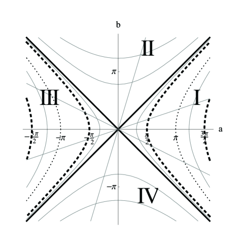
Figure 1: Regions of the perturbation amplitudes $\left(a,b\right)$-plane. Bisectrices of the coordinate angles separating the $\left(a,b\right)$-plane are presented by the thick solid lines. The singular hyperbolae $\rho_{1,3}=\pi/2+\pi n$ are presented by the thick dashed lines. Non-singular hyperbolae are presented by the thin solid lines. The hyperbolae $\rho_{1,3}=\pi n$ are presented by the thin dotted lines.

It is convenient to divide the plane $\left(a,b\right)$ into four regions separated by the coordinate angles bisectrices $a^{2}=b^{2}$ (see Fig. 1). We numerate these regions from I to IV.

III.1 Resonances: $a^{2}>b^{2}$

Let us consider at first the region I of the $\left(a,b\right)$-plane (see Fig. 1). It is useful to introduce there the hyperbolic variables$:$

$$a=\rho_{1}\cosh\psi_{1},\text{ \ \ }b=\rho_{1}\sinh\psi_{1}.$$ (35)

Then Eq. (34) takes the form:

$$J_{j-1/2}\left(Er_{0}\right)H_{j+1/2}^{\left(1\right)}\left(Er_{0}\right)+J_{j+1/2}\left(Er_{0}\right)H_{j-1/2}^{\left(1\right)}\left(Er_{0}\right)$$

$$=\tan\rho_{1}\left[\exp\left(\psi_{1}\right)J_{j-1/2}\left(Er_{0}\right)H_{j-1/2}^{\left(1\right)}\left(Er_{0}\right)-\exp\left(-\psi_{1}\right)J_{j+1/2}\left(Er_{0}\right)H_{j+1/2}^{\left(1\right)}\left(Er_{0}\right)\right].$$ (36)

Periodicity of tan$\rho_{1}$ allows us to restrict the analysis here by the segment $0\leq\rho_{1}\leq\pi.$ Consideration of only right half-plane of energies $\mathop{\mathrm{R}e}$ $E>0$ and $j=\pm 1/2,\pm 3/2,\ldots$will be suffice due to the symmetry Eq. (8).

For a fixed $\rho_{1},$ we can consider the asymptotic behavior at $\left|\psi_{1}\right|\rightarrow\infty.$ Eq. (36) asymptotically transforms into the equations

$$J_{j-1/2}\left(Er_{0}\right)H_{j-1/2}^{\left(1\right)}\left(Er_{0}\right)=0,\text{ \ \ \ }\psi_{1}\rightarrow\infty,$$ (37)

$$J_{j+1/2}\left(Er_{0}\right)H_{j+1/2}^{\left(1\right)}\left(Er_{0}\right)=0,\text{ \ \ \ }\psi_{1}\rightarrow-\infty.$$ (38)

Since the Hankel functions $H_{j\mp 1/2}^{\left(1\right)}\left(Er_{0}\right)$ have no roots in the right halfplane stegun , solutions $E_{n}^{\left(j\mp 1/2\right)}$of Eq. (37), Eq. (38) read

$$E_{n}^{\left(j-1/2\right)}=\lambda_{n}^{\left(j-1/2\right)}/r_{0},\text{ \ \ \ }\psi_{1}\rightarrow\infty,\text{ \ \ \ }n=1,2,\ldots$$ (39)

$$E_{n}^{\left(j+1/2\right)}=\lambda_{n}^{\left(j+1/2\right)}/r_{0},\text{ \ \ \ \ }\psi_{1}\rightarrow-\infty,\text{ \ \ }n=1,2,\ldots$$ (40)

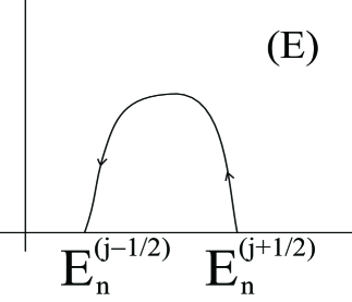
Figure 2: Schematic diagram of the arc-like resonance trajectory. $E_{n}^{\left(\lambda\pm 1/2\right)}$ are the roots of the Bessel functions $J_{j\pm 1/2}\left(r_{0}E\right).$

with $\lambda_{n}^{\left(j\mp 1/2\right)}$ being the roots of the Bessel functions $J_{j\mp 1/2}\left(z\right),$ which are real and tend to infinity. Thus we conclude that solutions of Eq. (36) are distributed on the arcuated curves beared on the real axis in the points $E_{n}^{\left(j\mp 1/2\right)}$ (see Fig. 2)

Notice that the case of $\left|\psi_{1}\right|\rightarrow\infty$ corresponds to $a^{2}\leftrightarrows b^{2}$ (see section II, Eq. (33). When we move along the non-singular hyperbolae $\rho_{1}\in\left(0,\pi/2\right)$ from $\psi_{1}=-\infty$ to $\psi_{1}=+\infty,$ the $n$-th arc-like curves are circumscribed in the complex plane of $E$ from the lying on the real axis point $E_{n}^{\left(j+1/2\right)}=r_{0}^{-1}\lambda_{n}^{\left(j+1/2\right)}$to the similar point $E_{n}^{\left(j-1/2\right)}=r_{0}^{-1}\lambda_{n}^{\left(j-1/2\right)}.$ When $\rho_{1}$ approaches $\pi/2$ (singular hyperbola), the ”arc” height tends to infinity. Moving along the arc-like curve takes place anti-clock-wise, when $\psi_{1}$ varies from $-\infty$ to $+\infty$. A transition between the points $E_{n}^{\left(j\pm 1/2\right)}$ corresponds to swapping of the upper and lower components of the wave function spinor amplitudes. However, crossing the singular hyperbolae $\pi/2$ leads to an essential rearrangement of the arc structure. Notably, the function $\tan\rho_{1}$ changes its sign and alternative combinations of nearest neighbor Bessel’s function roots are connected by arcs in order to satisfy the characteristic equation. Thus, the resonance arc-like curve begins in the point $E_{n}^{\left(j+1/2\right)}$ and moves clock-wise into the point $E_{n+1}^{\left(j-1/2\right)}$, when $\pi/2<\rho_{1}<\pi.$ A schematic picture of such transitions of arcs is presented in Fig. 3. Results of numerical calculations for $\rho_{1}\in\left(0,\pi\right)$ presented in Fig. 4 for $\rho_{1}\in\left(0,\pi/2\right)$ and in Fig. 5 for $\rho_{1}\in\left(\pi/2,\pi\right).$ They are in good qualitative agreement with our analytic consideration. A periodicity with the period $\Delta\rho_{1}=\pi$ takes place.

Motion along rays in the region I of the $\left(a,b\right)$-plane maps into closed resonance trajectories in the energy complex plane in the case of the ray lying in the upper half-plane. In the case of the ray lying in the lower half-plane we obtain repeating jumps from one resonance to the next one instead of the closed curves (see Fig. 6)..When the ray approaches the coordinate angle bisectrix, the closed curves diameter decreases so that the curves shrink into a point.

Consider now the left quarter (region III in Fig. 1):

$$a=-\rho_{3}\cosh\psi_{3},\text{ }b=-\rho_{3}\sinh\psi_{3}.$$ (41)

Then the characteristic equation reads

$$J_{j-1/2}\left(r_{0}E\right)H_{j+1/2}^{\left(1\right)}\left(r_{0}E\right)+J_{j+1/2}\left(r_{0}E\right)H_{j-1/2}^{\left(1\right)}\left(r_{0}E\right)$$

$$=\tan\rho_{3}\left[\exp\left(-\psi_{3}\right)J_{j+1/2}\left(r_{0}E\right)H_{j+1/2}^{\left(1\right)}\left(r_{0}E\right)-\exp\left(\psi_{3}\right)J_{j-1/2}\left(r_{0}E\right)H_{j-1/2}^{\left(1\right)}\left(r_{0}E\right)\right].$$ (42)

The asymptotic form of the equation at $\left|\psi_{3}\right|\longrightarrow\infty$ is following

$$J_{j-1/2}\left(r_{0}E\right)=0,\text{ }\psi_{3}\rightarrow\infty,$$

$$J_{j+1/2}\left(r_{0}E\right)=0,\text{ }\psi_{3}\rightarrow-\infty.$$

When $\psi_{3}$ varies from $-\infty$ to $+\infty$ circumscribing the hyperbola in the region III, we have motion from the roots of $J_{j+1/2}\left(r_{0}E\right)$ to the roots of $J_{j-1/2}\left(r_{0}E\right)$ in the energy complex plane (the same arc-form curves circumscribed anti-clock-wise or clock-wise respectively for $\rho_{3}\in(0,$ $\pi/2)$ or $\left(\pi/2,\pi\right)$). Numeric calculations are similar to the case of the region I; they confirm conclusions of our analysis.

An increase of the potential radius $r_{0}$ shifts the roots in the direction of the coordinate origin.

III.2 Resonances: $b^{2}>a^{2}$

Now we consider the region II in the $\left(a,b\right)$-plane (see Fig. 1). We introduce the hyperbolic variables here differently:

$$b=\rho_{2}\cosh\psi_{2},\text{ }a=\rho_{2}\sinh\psi_{2}.$$ (43)

The characteristic equation takes the form

$$J_{j-1/2}\left(r_{0}E\right)H_{j+1/2}^{\left(1\right)}\left(r_{0}E\right)+J_{j+1/2}\left(r_{0}E\right)H_{j-1/2}^{\left(1\right)}\left(r_{0}E\right)$$

$$=\left[\exp\left(\psi_{2}\right)J_{j-1/2}\left(r_{0}E\right)H_{j-1/2}^{\left(1\right)}\left(r_{0}E\right)+\exp\left(-\psi_{2}\right)J_{j+1/2}\left(r_{0}E\right)H_{j+1/2}^{\left(1\right)}\left(r_{0}E\right)\right]\tanh\rho.$$ (44)

One can see that in the limit of $a\leftrightarrows b$ we have the equation

$$J_{j-1/2}\left(r_{0}E\right)=0,\text{ \ \ \ }\psi_{2}\rightarrow\infty,$$

while for $a\leftrightarrows-b$ we have

$$J_{j+1/2}\left(r_{0}E\right)=0,\text{ \ \ \ }\psi_{2}\rightarrow-\infty.$$

Thus, the roots circumscribe arc-form curves clock-wise from the point $\lambda_{n}^{\left(j-1/2\right)}/r_{0}$ to $\lambda_{n}^{\left(j+1/2\right)}/r_{0}$ (see Fig. 7), while $\psi_{2}$ varies from $+\infty$ to $-\infty$ (motion along the upper hyperbolae in Fig. 1 anti-clock-wise).

Let us learn a limiting form of the arcs, when $\rho_{2}\longrightarrow\infty.$ As $\tanh\rho_{2}\longrightarrow 1,$ Eq. (44) takes the form

$$\left[\mathcal{J}_{j}\left(r_{0}E_{jn}\right)-\exp\left(-\psi_{2}\right)\right]\left[\mathcal{H}_{j}\left(r_{0}E_{jn}\right)-\exp\left(-\psi_{2}\right)\right]=0,$$ (45)

where $E_{jn}=E_{jn}^{\left(1\right)}-i\Gamma_{jn}/2$ is the complex root of the characteristic equation; we used the standard notions for the real and imaginary parts of the resonance energy.

Notice that roots of the second factor are not physical and must be ignored. Eq. (45) can be written in the form

$$\mathcal{J}_{j}\left(r_{0}\left(E_{jn}^{\left(1\right)}-i\Gamma_{jn}/2\right)\right)=\exp\left(-\psi_{2}\right),\text{ }\rho_{2}\longrightarrow\infty,$$ (46)

Since $\mathcal{J}_{j}\left(z\right)$ is real on the real axis, we have $\mathcal{J}_{j}\left(z\right)^{\ast}=\mathcal{J}_{j}\left(z^{\ast}\right)$ and, therefore, $\mathcal{J}_{j}\left(r_{0}\left(E_{jn}^{\left(1\right)}-i\Gamma_{jn}/2\right)\right)=\mathcal{J}_{j}\left(r_{0}\left(E_{jn}^{\left(1\right)}+i\Gamma_{jn}/2\right)\right)^{\ast}=\exp\left(-\psi_{2}\right).$ So we see that $E_{jn}^{\left(1\right)}+i\Gamma_{jn}/2$ is a root of Eq. (46) as well. Since the ends of the arc are simple zeros of the Bessel function, these two arcs coincide and are flat in this limit. Eq. (46) takes the form

$$\mathcal{J}_{j}\left(r_{0}E_{jn}^{\left(1\right)}\right)\equiv J_{j-1/2}/J_{j+1/2}=\exp\left(-\psi_{2}\right)=\sqrt{\left(b-a\right)/\left(b+a\right)},\text{ \ \ }b^{2}\gg a^{2}.$$ (47)

We see that the energy imaginary part is getting extremely small and the arcs approach the real axis segments $[\lambda_{n}^{\left(j-1/2\right)}/r_{0},$ $\lambda_{n}^{\left(j+1/2\right)}/r_{0}]$ so fast at $\rho_{2}\longrightarrow\infty$ that it is difficult to observe a presence of the imaginary part numerically. However, this process can be followed analytically. In order to investigate the limiting behavior of the energy imaginary part, we expand Eq. (44) for $\rho_{2}\longrightarrow\infty$ taking account of the asymptotics leading terms. In particular, the expansion $\tanh x\cong 1-\exp\left(-2x\right)+\ldots$ for $x\gg 1$ was used. Taking the real part of Eq. (44), we obtain after some algebra

$$\mathop{\mathrm{R}e}\mathcal{J}_{j}(r_{0}E_{jn})\left[1-\left(1-\exp(-2\rho_{2})\exp\left(\psi_{2}\right)\mathop{\mathrm{R}e}\mathcal{H}_{j}\left(r_{0}E_{jn}\right)\right)\right]$$

$$= -\mathop{\mathrm{R}e}\mathcal{H}_{j}\left(r_{0}E_{jn}\right)+\Gamma_{n}\mathcal{J}_{j}^{{}^{{}^{\prime}}}\left(r_{0}E_{jn}^{\left(1\right)}\right)\left(r_{0}/2\right)\left(1-\exp\left(-2\rho_{2}\right)\right)\exp\left(-\psi_{2}\right)\mathop{\mathrm{I}m}\mathcal{H}_{j}\left(r_{0}E_{jn}\right)$$

$$+\left(1-\exp\left(-2\rho_{2}\right)\right)\exp\left(-\psi_{2}\right).$$

Expanding this formula for small $\Gamma_{jn}$ we obtain in the leading order

$$r_{0}\Gamma_{jn}/2=-\frac{\exp\left(-\psi_{2}-2\rho_{2}\right)}{\mathcal{J}_{j}^{{}^{{}^{\prime}}}\left(r_{0}E_{jn}^{\left(1\right)}\right)}\cdot\frac{\mathop{\mathrm{R}e}\mathcal{H}_{j}\left(r_{0}E_{jn}^{\left(1\right)}\right)+\exp\left(-\psi_{2}\right)}{\mathop{\mathrm{I}m}\mathcal{H}_{j}\left(r_{0}E_{jn}^{\left(1\right)}\right)}.$$ (48)

Here $E_{jn}^{\left(1\right)}$ is determined from Eq. (47). It is seen from Eq. (48) that the resonance width $\Gamma_{jn}$ decreases exponentially at large $\rho_{2}.$

Returning to the initial notions we find:

$$r_{0}\Gamma_{jn} = 2\exp\left(-2\sqrt{b^{2}-a^{2}}\right)\frac{\sqrt{\left(b-a\right)/\left(b+a\right)}J_{j+1/2}^{2}}{J_{j+1/2}^{{\acute{}}}J_{j-1/2}-J_{j-1/2}^{{\acute{}}}J_{j+1/2}}$$ (49)

$$\cdot\frac{\mathop{\mathrm{R}e}\left[H_{j-1/2}^{\left(1\right)}/H_{j+1/2}^{\left(1\right)}\right]+\sqrt{\left(b-a\right)/\left(b+a\right)}}{\mathop{\mathrm{I}m}\left[H_{j-1/2}^{\left(1\right)}/H_{j+1/2}^{\left(1\right)}\right]},\text{ \ \ \ \ \ \ \ \ }b^{2}>>a^{2}$$

The obtained formula indicates that these resonances are extremely sharp for the case of small $\left|j\right|$ and, therefore, they can give a strong resonance scattering of electrons. Using the Bessel functions $J_{\nu},$ $H_{\nu}^{\left(1\right)}$ asymptotics for large $\nu$ stegun , we obtain the following estimate for the resonance width asymptotic at large $\left|j\right|:$

$$\Gamma_{jn}\sim\left(r_{0}^{-1}\right)\sqrt{\left(b-a\right)/\left(b+a\right)}\exp\left(-2\sqrt{b^{2}-a^{2}}\right)\left(\left|j\right|/e\right)^{\left|j\right|}.$$ (50)

This function catastrophically increases beginning from $\left|j\right|\sim 4.$ It means that the imaginary part of the energy is large for any realistic $\rho_{2}$ so that solutions with $j>4$ are not really sharp resonances and they will not contribute into the electron resonance scattering.

Results of numeric calculation for resonances in the case of $b^{2}>a^{2}$ are presented in Figs. 7 and 8. Approaching of arc-like resonance curves to the real axis segments, when $\rho_{2}$ increases, is shown in Fig. 7. Fig. 8 shows the resonance trajectory corresonding to a motion along the ray in the $\left(a,b\right)$-plane region II. When the radius increases, the trajectory approaches a point on the real axis.

The region IV (lower quarter) can be analyzed similarly using the hyperbolic variables:

$$b=-\rho_{4}\cosh\psi_{4},\text{ }a=-\rho_{4}\sinh\psi_{4}$$ (51)

An analisis of this region could be done similarly to the region II, but we omit it here since no qualitative distinction is observed in this case. Numerical results for the region IV are omitted by us as well because of this similarity.

So we have discussed a local behavior of the resonance trajectories within the chosen quarter in the $\left(a,\text{ }b\right)$-plane. Now we will consider the global behavior, when all quarters are passed along hyperbolae with the fixed hyperbolic radius $\rho.$ This process creates pairs of arc-form curves bearing on two common basing points lying on the real axis. These figures of eight are arranged at the $E$ complex plane symmetrically relative to the imaginary axis in the case of $m=0.$ Resonances move anti-clock-wise from the root $\lambda_{n}^{\left(j+1/2\right)}/r_{0}$ to the root $\lambda_{n}^{\left(j-1/2\right)}/r_{0}$ circumscribing the arc, when $\phi\in\left[-\pi/4,\text{ }\pi/4\right]$ When $\phi\in\left[\pi/4,\text{ }3\pi/4\right],$ a different arc appears. It connects the same points $\lambda_{n}^{\left(j+1/2\right)}$ and $\lambda_{n}^{\left(j-1/2\right)}$, but moving in the opposite direction (clock-wise). We obtain in result the figures-of-eight in the $E$-complex plane. This picture is repeated with the period $\Delta\phi=\pi$.

Such excursion around all quarters of the $\left(a,\text{ }b\right)$-plane can be carried out circumscribing the circles in the $\left(a,b\right)$-plane

$$a=\rho\cos\phi,\text{ }b=\rho\sin\phi.$$ (52)

One quarter after another is passed in this case too, but now the figures-of-eight do not touch the real energy axis anymore (see Fig. 9), i. e. all resonances belonging to this set have rather large widths. Numeric analysis confirms our prediction on the mapping of the circular excursion in the $\left(a,b\right)$ plane onto the energy plane. When the perturbation intensity $\rho$ is increased, the picture is getting more complicated: all the figures-of-eight are associating into a single whole (see Fig. 9 for large $\rho$). Notice that the resonance trajectory self-crossing points are fixed points relative to $\rho$ changes. !They correspond to resonance set, which do not change at motion along the ray $a=b.$

IV Gapped graphene

While the pristine graphene is gapless, a contact with the substrate can induce some narrow gap gap . That is why we study here bound and resonance states in the gapped graphene as well.

Let us consider the characteristic equation for the case of $m\neq 0.$ We introduce the dimensionless parameters:

$$\epsilon=E/m,\text{ }r_{0}m=r_{0}/r_{c}=\gamma,$$ (53)

where $r_{c}=1/m$ is the ”Compton radius” ($\hslash=1,$ $v_{F}=1).$ The characteristic equation for bound states Eq. (22) takes the form:

$$\sqrt{1-\epsilon^{2}}\left[I_{j-1/2}\left(z\right)K_{j+1/2}\left(z\right)-K_{j-1/2}\left(z\right)I_{j+1/2}\left(z\right)\right]$$ (54)

$$= T(a,b)\left[\left(1-\epsilon\right)\left(a-b\right)J_{j+1/2}\left(z\right)K_{j+1/2}\left(z\right)+\left(1+\epsilon\right)\left(a+b\right)I_{j-1/2}\left(z\right)K_{j-1/2}\left(z\right)\right],$$

where $z=\gamma\sqrt{1-\epsilon^{2}}.$ The perturbation radius $r_{0}$ value is of order of the lattice spacing $d,$ while the ”Compton” radius $r_{c}$ is rather large: $r_{c}>>d:$ $\hslash/\left(m_{0}v_{F}\right)\sim 10^{-8}$ $cm$ even for the bare electron mass $m_{0}$; the real effective mass at the band extrema can be estimated as $10^{-1}-10^{-2}$ of $m_{0}$. Therefore, the actual value of $\gamma$ is less than unity.

We consider here some general properties of the bound states electronic spectrum resulting from the characteristic equation (54) and the effect of non-vanishing gap on the resonance states. Results of the numerical solution will be presented too.

IV.1 Bound states: $a^{2}>b^{2}$

Let us assume at first $j=1/2.$ We consider Eq. (54) for the energy situated in the gap $\epsilon^{2}<1$. We use the Bessel functions limiting forms for the states lying near the gap edges stegun

$$I_{\nu}(z)\sim\left(z/2\right)^{\nu}\frac{1}{\Gamma\left(\nu+1\right)},\text{ }K_{0}\left(z\right)\sim-\log z,\text{ }K_{\nu}\left(z\right)\sim\frac{1}{2}\Gamma\left(\nu\right)\left(z/2\right)^{-\nu},$$ (55)

in order to transform the characteristic equation (54). Here $\Gamma\left(\nu\right)$ is the gamma function. We obtain a simple relation for small $z.$

$$1+\left(\gamma^{2}/4\right)\left(1-\epsilon^{2}\right)\log\left(\gamma\sqrt{1-\epsilon^{2}}\right)$$ (56)

$$\cong \gamma\frac{\tan\sqrt{a^{2}-b^{2}}}{\sqrt{a^{2}-b^{2}}}\left[\left(1-\epsilon\right)\left(a-b\right)/4-\left(1+\epsilon\right)\left(a+b\right)\log\left(\gamma\sqrt{1-\epsilon^{2}}\right)\right].$$

Formulae like Eq. (56) determine a map from the plane $\left(a,b\right)$ onto the complex energy plane; in the case of bound states the map is carried out onto the real energy axis segment $-1<\epsilon<1.$Now we consider the asymptotic energy level behavior near the upper edge of the gap $\epsilon\longrightarrow 1.$ Eq. (56) takes the asymptotic form:

$$1\cong-\gamma\frac{\tan\sqrt{a^{2}-b^{2}}}{\sqrt{a^{2}-b^{2}}}\left(a+b\right)\log\left[2\gamma^{2}\left(1-\epsilon\right)\right].$$ (57)

Therefore, we can write

$$1-\epsilon\cong\left(2\gamma^{2}\right)^{-1}\exp\left[-\left(1/\gamma\right)\frac{1}{a+b}\cdot\frac{\sqrt{a^{2}-b^{2}}}{\tan\sqrt{a^{2}-b^{2}}}\right].$$ (58)

It is clear that $\epsilon\longrightarrow 1$  if $a+b\longrightarrow+.$ $0.$ This result conforms the well known general property of the two-dimensional quantum systems: a threshold for creation of the bound state is absent for $j=1/2$.

Formula (58) can be rewritten in the hyperbolic variables in the region I (see Eq. (35) as follows

$$1-\epsilon\cong\left(2\gamma^{2}\right)^{-1}\exp\left[-1/\left(\gamma\exp\left(\psi_{1}\right)\tan\rho_{1}\right)\right].$$ (59)

It is seen from the last formula that $\epsilon\longrightarrow 1$, when $\rho_{1}\longrightarrow\pi n+0$ (where $n=1,$ $2\ldots)$, i. e. the $\epsilon=1$ ”fronts” approach the hyperbolae $\rho_{1}=\sqrt{a^{2}-b^{2}}\longrightarrow\pi n+0.$

Let us study now a behavior of the bound state trajectory near the lower band edge. Using Eq. (56) we conclude that when $\epsilon\longrightarrow-1,$ the following relation holds:

$$1\cong\gamma\tan\left(\rho_{1}\right)\exp\left(-\psi_{1}\right)\left(1-\epsilon\right)/4.$$ (60)

This equation shows, how the bound states trajectory approaches the lower edge of the gap. Putting $\epsilon=-1$ we obtain the equation, which determines the $\epsilon=-1$ boundary lines in the $\left(a,b\right)$-plane, separating the domains of the bound states:

$$\tan\rho_{1}=2\exp\psi_{1}/\gamma.$$ (61)

When $\psi_{1}\longrightarrow+\infty$ along one of these lines, $\rho_{1}\longrightarrow\pi/2+\pi n-0,$ $n=0,1,\ldots$. The line $n=0$ crosses the abscissa axis in the point (see Eq. (60)):

$$b_{0}=0,\text{ }a_{0}=\arctan\left(2/\gamma\right).$$ (62)

Then this curve crosses the bisectrix $a+b=0$ in the point $a_{1}=1/\gamma,$ $b_{1}=-1/\gamma.$ Any point situated in the domain restricted at the left by the bisectrix $a-b=0$ and at the right by the line Eq. (61) ($\epsilon=-1$ ”front”) (which asymptotically approaches the hyperbola $\rho_{1}=\pi/2-0,$ $\psi_{1}\longrightarrow+\infty$), gives a solution of the characteristic equation lying in the gap $\left|\epsilon\right|<1$ that is an eigenvalue of our problem. A motion from the bisectrix $a+b=0$ to the curve Eq. (61) in the region I of the $(a,b)$-plane is mapped to the motion from the upper to lower edges in the energy gap.

Other domains with $n=1,2,\ldots,$ lie between approaching the hyperbolae $\rho_{1}=\pi n-0$ curves ($\epsilon=1$ ”front”, $\left|\psi_{1}\right|\longrightarrow\infty$) and the $\epsilon=-1$ ”front”, approaching the hyperbolae $\rho_{1}=\pi/2+\pi n-0$ at $\psi_{1}\longrightarrow+\infty$ and the hyperbolae $\rho_{1}=\pi n+0$ at $\psi_{1}\longrightarrow-\infty.$ These lines boarder the countable set of domains in the $\left(a,b\right)$-plane, where the bound states exist. When we move along the lying in the region I ray beginning in the coordinate origin in the direction of the $\rho_{1}^{2}=a^{2}-b^{2}$ increase, we cross this set of domains so that every time the bound states trajectory starts at $\epsilon=1$ and terminates at $\epsilon=-1.$

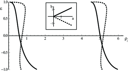
Figure 10: Eigenvalue dependence on the radial coordinate $\rho_{1}$ in the region I for two angle magnitudes: solid line $\phi=\pi/6,$ dashed line $\phi=-\pi/6.$In the inset: Two rays in the $(a,b)$-plane with the above angle values.

A dependence of the bound state energy on the radius $\rho_{1},$ at the motion along the rays in the $\left(a,b\right)$-plane (see inset to Fig. 10) was investigated numerically in the case of $a^{2}>b^{2}$. The motion between the coordinate origin and the first $\epsilon=-1$ ”front” maps into the mildly sloping  transition between the $\epsilon=1$ and $\epsilon=-1$ edges of the gap (solid line) and the sharp sloping transition respectively for the rays in the upper and lower half-planes of the $\left(a,b\right)$-plane (first pair of the curves). The second and so on pairs of curves show similar transitions between the domain boundaries.

Now we consider the region III. Let us return to Eq. (56) that is valid near the band edges and everywhere inside the gap if $\gamma<<1.$ Using the hyperbolic variables Eq. (41) we can write for the bound states near the upper edge $\epsilon=+1:$

$$1-\epsilon\cong\left(2\gamma^{2}\right)^{-1}\exp\left[\frac{\exp\left(\psi_{3}\right)}{\gamma\tan\rho_{3}}\right].$$ (63)

Eq. (63) is satisfied near the hyperbolae $\rho_{3}=\pi n-0$ (then $\tan\rho_{3}\longrightarrow-0).$ This determines the $\epsilon=1$ ”front” of domains containing the eigenvalues. The $\epsilon=1$ ”fronts” are formed by the approaching the hyperbolae $\rho_{3}=\pi n-0$, ($n=1,2,\ldots)$ at $\left|\psi_{3}\right|\longrightarrow+\infty.$ Therefore, we have the exponential approaching of the energy level to the upper band edge in the region III similarly to the region I.

The $\epsilon=-1$ ”fronts” Eq. (61)

$$\tan\rho_{3}=-\left(2/\gamma\right)\exp\psi_{3}$$

approach the hyperbolae $\rho_{3}=\pi n-0,$ when $\psi_{3}\longrightarrow-\infty,$ and hyperbolae $\rho_{3}=-\pi/2+\pi n+0,$ when $\psi_{3}\longrightarrow+\infty,$ $n=1,2,\ldots.$

IV.2 Bound states: $b^{2}>a^{2}$

Let us consider the region II in the $\left(a,b\right)$-plane.The approximate characteristic equation Eq. (56) for the states near the band edges in the case of $b^{2}>a^{2}$ reads:

$$1+\left(\gamma^{2}/4\right)\left(1-\epsilon^{2}\right)\log\left(\gamma\sqrt{1-\epsilon^{2}}\right)$$ (64)

$$\cong \gamma\frac{\tanh\sqrt{b^{2}-a^{2}}}{\sqrt{b^{2}-a^{2}}}\left[\left(1-\epsilon\right)\left(a-b\right)/4-\left(1+\epsilon\right)\left(a+b\right)\log\left(\gamma\sqrt{1-\epsilon^{2}}\right)\right].$$

We obtain for the energy near the upper band gap edge:

$$1-\epsilon\cong\left(2\gamma^{2}\right)^{-1}\exp\left[-\left(1/\gamma\right)\frac{1}{a+b}\cdot\frac{\sqrt{b^{2}-a^{2}}}{\tanh\sqrt{b^{2}-a^{2}}}\right].$$

Thus, the $\epsilon=1$ ”front” approaches the bisectrix $a+b\longrightarrow 0$ exponentially. We introduce here the variables

$$b=\rho_{2}\cosh\psi_{2},\text{ }a=\rho_{2}\sinh\psi_{2}.$$ (65)

Then Eq. (64) takes the form

$$1+\left(\gamma^{2}/4\right)\left(1-\epsilon^{2}\right)\log\left(\gamma\sqrt{1-\epsilon^{2}}\right)$$ (66)

$$\cong -\gamma\tanh\rho_{2}\left[\left(1-\epsilon\right)\exp\left(-\psi_{2}\right)/4+\left(1+\epsilon\right)\exp\left(\psi_{2}\right)\log\left(\gamma\sqrt{1-\epsilon^{2}}\right)\right].$$

We obtain for the energies near the upper band edge $\epsilon\longrightarrow 1$:

$$1-\epsilon\cong 1/\left(2\gamma^{2}\right)\exp\left[-\frac{\exp\left(-\psi_{2}\right)}{\gamma\tanh\rho_{2}}\right]$$ (67)

Thus, the $\epsilon=1$ ”front” approaches the bisectrix $a+b=0$ at $\rho_{2}\longrightarrow 0.$ There is no ”front” at the bisectrix $a-b=0$ as it was shown above. Eq. (66) can be rewritten for $\rho_{2}\longrightarrow\infty:$

$$\left[1+\left(\gamma/4\right)\left(1-\epsilon\right)\exp\left(-\psi_{2}\right)\right]\left[1+\gamma\left(1+\epsilon\right)\exp\left(\psi_{2}\right)\log\left(\gamma\sqrt{1-\epsilon^{2}}\right)\right]\cong 0.$$ (68)

Therefore,

$$\gamma\left(1+\epsilon\right)\exp\left(\psi_{2}\right)\log\left(\gamma\sqrt{1-\epsilon^{2}}\right)\cong-1.$$ (69)

Eq. (69) is satisfied if $\epsilon\longrightarrow-1$ and $\psi_{2}\longrightarrow+\infty.$ Therefore, the $\epsilon=-1$ ”front” approaches the bisectrix $a-b=0,$ if $\rho_{2}\longrightarrow\infty.$This ”front” lies in the region I (see above). Thus, a motion in the region II of the plane $\left(a,b\right)$ from the bisectrix $a+b=0$ to the bisectrix $a-b=0$ corresponds to a motion of the energy eigenvalue from the upper band edge $\epsilon=1$ to the lower band edge $\epsilon=-1$, when $\rho_{2}>>1.$

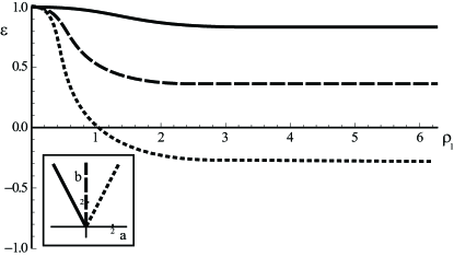
Figure 11: Eigenvalue dependence on the radial coordinate $\rho_{2}$ in the region II for three angle values (corresponding rays are shown in the inset): solid lines $\phi=2\pi/3,$ dashed lines $\phi=\pi/2,$ dotted lines $\phi=-2\pi/3.$

A dependence of the bound state energy on the radius $\rho_{2},$ at the motion along the rays in the $\left(a,b\right)$-plane (see inset to Fig. 11) was investigated numerically in the case of $a^{2}<b^{2}$. The motion along the ray maps into the monotone transition of the energy level from the band gap edge $\epsilon=1$ to the constant situated in the gap. Motion along the ray in the right half-plane maps into the faster energy dependence and with lower asymptotic energy value, than in the case of the ray in the left half-plane. When the ray approaches the bisectrix $a-b=0$, the asymptotic value tends to $\epsilon=-1.$

Let us consider now solutions of the characteristic equation near the band edges for the parameters $a,b$ in the region IV. We introduce the hyperbolic variables (see Eq. (51)).

Then Eq. (64) can be approximately written in the form:

$$1+\left(\gamma^{2}/4\right)\left(1-\epsilon^{2}\right)\log\left(\gamma\sqrt{1-\epsilon^{2}}\right)$$ (70)

$$\cong \gamma\tanh\rho_{4}\left[\left(1-\epsilon\right)\exp\left(-\psi_{4}\right)/4+\left(1+\epsilon\right)\exp\left(+\psi_{4}\right)\log\left(\gamma\sqrt{1-\epsilon^{2}}\right)\right].$$

The line

$$1\cong\left(\gamma/2\right)\exp\left(-\psi_{4}\right)\tanh\rho_{4}$$ (71)

corresponds to the $\epsilon=-1$ ”front” in the region IV. This line is a continuation of the line Eq. (61); they meet in the point $a=-b=1/\gamma.$ The line Eq. (71) turns into the asymptotic at $\rho_{4}\longrightarrow\infty:$

$$\psi_{4}\longrightarrow-\log\left(2/\gamma\right).$$ (72)

Let us transform Eq. (70) in the limit of $\rho_{4}\longrightarrow\infty:$

$$\left[1-\left(\gamma/4\right)\left(1-\epsilon\right)\exp\left(-\psi_{4}\right)\right]\left[1-\gamma\left(1+\epsilon\right)\exp\left(\psi_{4}\right)\log\left(\gamma\sqrt{1-\epsilon^{2}}\right)\right]\cong 0.$$ (73)

The ”front” $\epsilon\longrightarrow 1$ equation takes the form

$$1-\epsilon\cong\left(4/\gamma\right)\exp\left(\psi_{4}\right)$$ (74)

Thus, the ”front” $\epsilon\longrightarrow 1$ approaches the bisectrix $b+a=0$ asymptotically, when $\psi_{4}\longrightarrow-\infty.$ Therefore, a motion from the line Eq. (72) to the bisectrix $b+a=0$ in the $\left(a,b\right)$ plane is mapped to a motion from the lower edge of the gap to the upper one when $\rho_{4}>>1.$

If $\gamma$ increases, we conclude from Eq. (72) that the second front $1+\epsilon\longrightarrow 0$ moves to the bisectrix $b-a=0,$ i. e. an increase of the mass widens the domain of the region IV, where the eigenvalues exist; it fills all region IV in the extreme limit.of large $\gamma.$ Notice that this case is not realistic for an impurity problem, but can be important for the quantum dot case matulis .

When $\gamma<<1,$ it is seen from Eq. (72) that the ”front” $1+\epsilon\longrightarrow 0$ tends to the ”front” $1-\epsilon\longrightarrow 0$ at $\psi_{4}\longrightarrow-\infty,$ i. e. the fronts tend to merge, when the gap tends to zero.

Thus, our analysis shows that there is a countable set of eigenvalue domains in the case $a^{2}>b^{2}.$ The boundaries of these domains approach the hyperbolae described above. In the case of $b^{2}>a^{2},$ we have a saturation instead of periodicity, when radius increases.

IV.3 Bound states for higher angular momenta

Let us consider now the eigenvalue spectrum for the angular momentum $j=3/2,$for instance, when the parameters $a,$ $b$ lie in the regions I and II.. Using the Bessel functions expansion for small arguments (55), Eq. (54) can be written as follows:

$$1/\gamma-\gamma\left(1-\epsilon^{2}\right)/12=T\left(a,b\right)\left[\left(a-b\right)\left(1-\epsilon\right)/12+\left(a+b\right)\left(1+\epsilon\right)/4\right].$$ (75)

In the region I, this equation takes the form

$$1/\gamma-\gamma\left(1-\epsilon^{2}\right)/12=\tan\rho_{1}\left[\left(1-\epsilon\right)\exp\left(-\psi_{1}\right)/12+\left(1+\epsilon\right)\exp\left(\psi_{1}\right)/4\right].$$ (76)

The ”fronts” $\epsilon\longrightarrow 1$ have the form

$$\tan\rho_{1}=\left(2/\gamma\right)\exp\left(-\psi_{1}\right).$$ (77)

We have asymptotically:

$$\rho_{1}\left(\psi_{1}\right)\longrightarrow\left\{\begin{array}[]{c}\pi/2+\pi n-0\text{ \ \ \ \ for\ }\psi_{1}\longrightarrow-\infty,\\ \\ \pi n+0\text{ \ \ \ for }\psi_{1}\longrightarrow\infty,\end{array}\text{ \ \ }n=1,2,\ldots\right.$$ (78)

The ”fronts” $\epsilon\longrightarrow-1$ have the form

$$\tan\rho_{1}=\left(6/\gamma\right)\exp\left(\psi_{1}\right).$$ (79)

Thus we have the lines

$$\rho_{1}\left(\psi_{1}\right)\longrightarrow\left\{\begin{array}[]{c}\pi n+0\text{ \ \ \ \ for\ }\psi_{1}\longrightarrow-\infty,\\ \\ \pi/2+\pi n-0\text{ \ \ \ for }\psi_{1}\longrightarrow\infty.\end{array}\text{ \ \ }n=1,2,\ldots\right.$$ (80)

The ”fronts” Eq. (77) ($\epsilon\longrightarrow 1)$, Eq. (79) $\left(\epsilon\longrightarrow-1\right)$ cross for the first time the abscissa axis respectively in the points

$$a_{1} = \arctan\left(2/\gamma\right),\text{ \ \ }b_{1}=0$$ (81)

$$a_{2} = \arctan\left(6/\gamma\right).$$ (82)

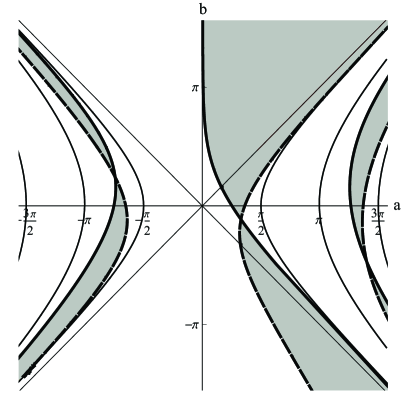
Figure 13: Diagram of bound states for $j=3/2$ and $\gamma=2.$ ”Fronts” $\epsilon=+1$ are shown by solid lines, ”fronts” $\epsilon=-1$ are shown by dashed lines. Thin solid line hyperbolae are asymptotes of the ”fronts”..

Therefore, a motion from the point $a_{1}$ to the point $a_{2}$ maps into a motion from $\epsilon=1$ to $\epsilon=-1.$ More than that, having in mind a continuous dependence of solutions on the parameters $a$ and $b$ the ”fronts” Eq. (77), Eq. (79) obtained from the asymptotic equation (76) cross one another. This prediction is confirmed by the numerical calculations (see Fig. 13). Exclusively fast dependence of the energy eigenvalues on the parameters $a$ and $b$ will be observed in the vicinity of the crossing point.

Let us consider now the region II. We have here from Eq. (75):

$$1/\gamma-\gamma\left(1-\epsilon^{2}\right)/12=\tanh\rho_{2}\left[-\left(1-\epsilon\right)\exp\left(-\psi_{1}\right)/12+\left(1+\epsilon\right)\exp\left(\psi_{1}\right)/4\right].$$ (83)

The ”front” $\epsilon\longrightarrow 1$ is given by the equation

$$\tanh\rho_{2}=\left(2/\gamma\right)\exp\left(-\psi_{2}\right).$$ (84)

Since $0\leq\tanh\rho_{2}\leq 1$  $\left(\rho_{2}\geq 0\right),$ we have

$$\psi_{2}\geq-\log\left(\gamma/2\right).$$ (85)

The domain, where the energy eigenvalues exist in the case of $\gamma=2,$ is bounded by the positive half-axis $b$ and the first quadrant bisectrix. When $\gamma<2$ and decreases, the ”front” $\epsilon=1$ turns about the coordinate origin from the ordinate axis approaching the first quadrant bisectrix. The eigenvalues domain is narrowing in result. When $\gamma>2$ and increases, this boundary turns anti-clock-wise approaching the second quadrant bisectrix. When $\psi_{2}\longrightarrow\infty,$ Eq. (83) can be satisfied only if

$$1+\epsilon=4/\left(\gamma\tanh\rho_{2}\right)\exp\left(-\psi_{2}\right),\text{ \ \ }\psi_{2}\longrightarrow\infty$$ (86)

We have for $\rho_{2}\longrightarrow\infty$ (higher hyperbolae):

$$1+\epsilon=\left(4/\gamma\right)\exp\left(-\psi_{2}\right),\text{ \ \ }\psi_{2}\longrightarrow\infty.$$ (87)

When $\psi_{2}$ is fixed, the asymptotic magnitude of the eigenvalue $\epsilon_{as}$ at $\rho_{2}\longrightarrow\infty$ can be found from the quadratic equation

$$\epsilon_{as}^{2}-\gamma^{-1}\left[6\exp\left(\psi_{2}\right)+2\exp\left(-\psi_{2}\right)\right]\epsilon_{as}-1+12/\gamma^{2}+\left(2/\gamma\right)\exp\left(-\psi_{2}\right)-\left(6/\gamma\right)\exp\left(\psi_{2}\right)=0.$$ (88)

The domain of eigenvalues in the region IV is narrower in the case of $j=3/2$, than for $j=1/2$ similarly to the region II. Generically, an increase of $j$ at fixed $\gamma$ leads to narrowing of the eigenvalues existence domains.

The case of higher angular momenta $j=5/2,\ldots$ can be analyzed similarly. The energy discrete eigenvalues exist for all $j,$ but in opposite to the case of $j=1/2,$ there is a threshold for the bound state appearing at the upper edge of the gap. Existence of bound states for all higher angular momenta is a specific feature of the delta function perturbation.

The states with $j<0$ can be easily obtained with a use of the symmetry transformation Eq. (8).

IV.4 Diagram of the bound states

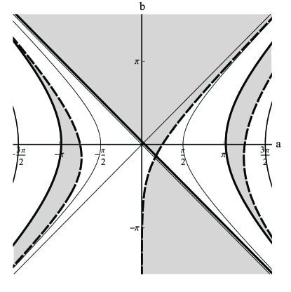
Figure 12: Diagram of bound states for $j=1/2$ and $\gamma=2.$ ”Fronts” $\epsilon=+1$ are shown by solid lines, ”fronts” $\epsilon=-1$ are shown by dashed lines. Thin solid line hyperbolae are asymptotes of the ”fronts”.

General results of mathematical and numerical analysis for a distribution of bound states for $j=1/2$ and $j=3/2$ are presented respectively in Figs. 12, 13. Shaded domains represent basines of the bound states existence. The thick lines correspond to the upper edge of the band gap $\epsilon=+1$, while the thin ones represent the lower edge $\epsilon=-1.$

In the case of $j=1/2,$ domain boundaries approach asymptotically the hyperbolae. One crossing point of boundaries can be seen. Therefore, we have one twisted domain in this case. Notice that this crossing looks so in a projection onto the $\left(a,b\right)$-plane. A  three-dimensional picture of this feature is shown.in Fig. 13: it is seen that the ”fronts” $\epsilon=\pm 1$ lie at different ”floors” so that the crossing curves in the plane curves appear to be skew ones.

Notice that our diagrams of states are obtained assuming single-valued dependence of the bound state energy on the parameters $a$ and $b$. This is true everywhere in the $\left(a,b\right)$-plane except very small islands near the domain boundaries (see Fig. 10 of this paper and our work we , where the twisting point neighborhood was analyzed numerically).

In the case of $j=3/2,$the bound state existence domains are getting narrower, a number of the boundaries crossing points increases. The diagram of states for higher $j$ is given us in Ref. we .

IV.5 Resonances: $m>0$

It is necessary to return now to Eq. (31) written in terms of non-modified Bessel’s functions. We consider here an effect of non-zero bandgap upon the resonance states. It is convenient to re-write Eq. (31) using the Bessel function explicitly (see eq (32)) and choosing $\alpha=1.$ We analyze here resonances for the parameters values lying in the region I as an example.

Introducing the hyperbolic coordinates according to Eq. (35) and using the dimensionless parametrization Eq. (53) , we can write

$$\left[J_{j-1/2}\left(\varsigma\right)H_{j+1/2}^{\left(1\right)}\left(\varsigma\right)+J_{j+1/2}\left(\varsigma\right)H_{j-1/2}^{\left(1\right)}\left(\varsigma\right)\right]$$ (89)

$$= -\tan\rho_{1}\left[\sqrt{\left(\epsilon-1\right)/\left(\epsilon+1\right)}\exp\left(-\psi_{1}\right)J_{j+1/2}\left(\varsigma\right)H_{j+1/2}^{\left(1\right)}\left(\varsigma\right)\right.$$

$$+\left.\sqrt{\left(\epsilon+1\right)/\left(\epsilon-1\right)}\exp\left(\psi_{1}\right)J_{j-1/2}\left(\varsigma\right)H_{j-1/2}^{\left(1\right)}\left(\varsigma\right)\right],$$

$$\mathop{\mathrm{R}e}E > 0,\text{ }j=\pm 1/2,\pm 3/2,\ldots,$$

where $\varsigma=\gamma\sqrt{\epsilon^{2}-1}.$ If $\psi_{1}\longrightarrow\pm\infty$ (asymptotical approach to the bisectrix), we have for the roots

$$J_{j\mp 1/2}\left(\varsigma\right)=0,\text{ \ \ }\psi_{1}\longrightarrow\pm\infty,$$ (90)

since the roots of the equation $H_{j\pm 1/2}^{\left(1\right)}\left(\varsigma\right)=0$ are extraneous ones. Solving Eq. (90), we obtain the Bessel function roots $\lambda_{n}^{\left(j\mp 1/2\right)}.$ Therefore,

$$\epsilon_{n}^{\left(j\mp 1/2\right)}=\sqrt{1+\left(\lambda_{n}^{\left(j\mp 1/2\right)}/\gamma\right)^{2}},\text{ \ \ }\psi_{1}\longrightarrow\pm\infty$$ (91)

This formula can be written in the form:

$$E_{n}^{\left(j\mp 1/2\right)}=\sqrt{m^{2}+\left(\lambda_{n}^{\left(j\mp 1/2\right)}/r_{0}\right)^{2}}$$ (92)

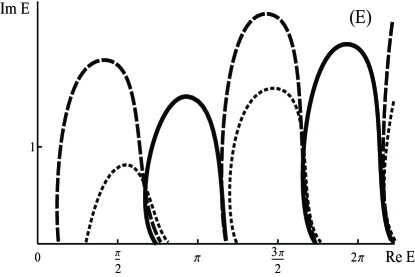
Figure 14: Arc-like resonance trajectory dependence on the mass (gap) value. Solid lines: $m=0,$ dashed lines: $m=0.5,$ dotted line $m=1.0.$

We see that appearing of non-zero mass shifts ”arc’s” bearing points relative to the positions, determined by Eqs.. (39), (40), in the direction of the energy increase (see Fig. 14). This shift is essential only for small $n$ since $\lambda_{n}^{\left(j\mp 1/2\right)}$ increases fast with $n$ increasing. When $m\neq 0,$ a distribution of signs of Eq. (89) right-hand-side for various $m$ values at fixed $\rho_{1}$ is complicated. Arcs, in result, can be formed both clock-wise and anti-clock depending on the $m$ value.

We have analyzed the resonances for the region I; the dependence of the resonances distribution on the parameter $\gamma=r_{0}m$ in other regions can be considered similarly.

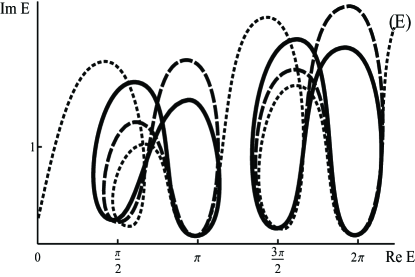
Figure 15: Figure-of-eight resonance trajectory dependence on the mass (gap) value. Solid lines: $m=0,$ dashed lines: $m=0.25,$ dotted line $m=0.5.$

We studied in the previous section a motion of resonances along the figure-of-eight curves in the case of $m=0$, when the parameters $a,b$ are varied along the circles Eq.(52) with various $\rho$ values. In the non-zero gap case, we have found that a large enough mass destructs the figure-of-eight structure for $\rho$ fixed; these figures associate into a whole complicated aggregate (see Fig. 15).

V Conclusion

In conclusion, we considered the bound and resonance electronic states for the two-dimensional Dirac equation with the short-range perturbation. The short-range perturbation is approximated by the delta function $\delta\left(r-r_{0}\right)$ with different amplitudes in the upper and lower electronic bands. We have in result local perturbations of the potential-like and mass-like types.respectively with amplitudes $a$ and $b$.

We derived the characteristic equations for the bound and resonance states. The characteristic equation is presented in forms convenient both for an analysis of the bound and resonance states. Energy levels behavior in dependence on the perturbation amplitudes was investigated both analytically and numerically. A general picture of the electronic spectrum dependence on the potential, and mass local perturbation is considered for various mass and angular momentum values; the results are presented as diagrams in the $\left(a,b\right)$-plane. Absence of a threshold for forming of the bound state in the vicinity of the upper bandgap edge is obtained for the lower angular momenta $\left|j\right|=1/2$ which is in accord with the general principles of quantum mechanics for the dimension 2+1.

A qualitative distinction of $a^{2}>b^{2}$ and $a^{2}>b^{2}$ cases is shown. A countable set of eigenvalues existence domains in the $\left(a,b\right)$-plane is present in the former case, while monotonic approaching to the asymptote takes place,  when $b^{2}-a^{2}\longrightarrow\infty$. in the latter one. Positions of asymptotes are determined by the parameter $\tanh^{-1}\left(b/a\right).$ Higher angular momenta are investigated as well. Twisted eigenvalue domains with crossing boundaries are found. Domains of eigenvalues are narrowing with the angular momentum increase and at the mass value fixed. A zero-energy solution with vanishing imaginary part exists in the zero-gap case.This solution has to be considered as a limit at $m\longrightarrow 0.$

Behavior of resonances depends essentially on the sign of $\left(a^{2}-b^{2}\right).$ When $a^{2}>b^{2},$ resonance trajectories in the energy complex plane have a form of closed curves circumscribed periodically at moving from the coordinate origin to infinity in the ($a,b)$-plane. Motion along the hyperbolae $\sqrt{a^{2}-b^{2}}=const$ maps onto the countable set of arc-like trajectories in the energy complex plane. These arcs bear on the real axis; positions of the bearing points are exactly determined by the Bessel function roots. When $b^{2}-a^{2}>0,$ an increase of $b^{2}-a^{2}$ forces the arcs to get flatter so that if $b^{2}-a^{2}\longrightarrow\infty,$ the arcs asymptotically nestle up to the real axis. The resonance width is exponentially small in this case. For higher angular momenta $j,$ the rate of this decrease is getting small due to the factor $\left|j\right|^{\left|j\right|}.$ Therefore, higher spherical harmonics do not contribute into the resonance scattering.

Two kinds of the non-zero mass effect on the resonances behavior were found. Firstly, positions of arc-bearing points shift. This effect is particularly essential for lower roots. Secondly, eight-like figures resulted from mapping of the circular motion in the $\left(a,b\right)$-plane onto the energy plane transform into large aggregates.

The carried out analysis allowed us to describe both qualitatively and quantitatively a distribution of the bound and resonance states in the energy complex plane for any chosen distribution of the perturbation amplitudes $a$ and $b$ and for various magnitudes of the mass and momentum. The obtained results can be useful for understanding of the graphene electronic properties.

Figure captions

Figure 3: Recommuting of the arc system in the region I, when $\rho_{1}$ crosses the singular hyperbolae $\rho_{1}=\pi/2+\pi n$, $n=0,1\ldots$
(a) $\pi n<\rho_{1}<\pi/2+\pi n.$
(b) $\pi/2+\pi n<\rho_{1}<\pi\left(n+1\right).$

Figure 4: Numerically calculated resonance trajectories for various $\rho_{1}$ values in the region I. Solid lines: $\rho_{1}=0.8,$ dashed lines: $\rho_{1}=1.4,$ dotted line $\rho_{1}=2.0.$
In the inset: Hyperbola paths in the $\left(a,b\right)$-plane.
In the body of figure: Maps of the above paths onto the resonances trajectories in the energy complex plane.

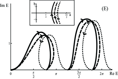
Figure 5: Numerically calculated resonance trajectories for various $\rho$ values in the region I. Solid lines: $\rho_{1}=2.5,$ dashed lines: $\rho_{1}=3.0,$ dotted grey lines $\rho_{1}=3.5.$
In the inset: Hyperbola paths in the $\left(a,b\right)$-plane.
In the body of figure: Maps of the above paths onto the resonances trajectories in the energy complex plane.

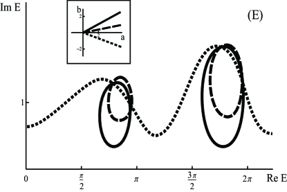
Figure 6: Numerically calculated resonance trajectories for motion along the rays in the $(a,b)$-plane in the region I. Solid lines: $\phi=\pi/7,$ dashed lines: $\phi=\pi/16,$ dotted lines: $\phi=-\pi/10.$
In the inset: Rays in the $\left(a,b\right)$-plane.
In the body of figure: Resonance trajectories in the energy complex plane.

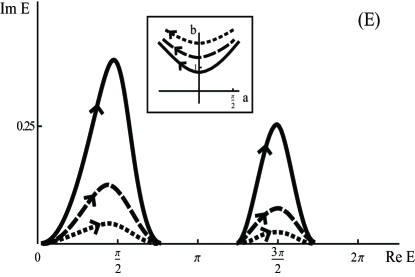
Figure 7: Numerically calculated resonance trajectories for various $\rho_{2}$ values in the region II. Solid lines: $\rho_{2}=0.8,$ dashed lines: $\rho_{2}=1.4,$ dotted lines $\rho_{2}=2.0.$
In the inset: Hyperbola paths in the $\left(a,b\right)$-plane.
In the body of figure: Maps of the above paths onto the resonances trajectories in the energy complex plane.

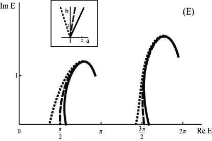
Figure 8: Numerically calculated resonance trajectories for motion along the rays in the $(a,b)$-plane in the region II. Solid lines: $\phi=5\pi/14,$ dashed lines: $\phi=7\pi/16,$ dotted lines $\phi=3\pi/5.$
In the inset: Rays in the $\left(a,b\right)$-plane.
In the body of figure: Corresponding resonance trajectories in the energy complex plane.

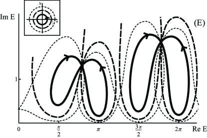
Figure 9: Numerically calculated resonance trajectories for motion along the circles in the $(a,b)$-plane. Solid lines: $\rho=0.8,$ dashed lines $\rho=1.4,$ dotted lines $\rho=2.0.$
In the inset: Circles in the $\left(a,b\right)$-plane.
In the body of figure: Corresponding figure-of-eight resonance trajectories in the energy complex plane.

References

- (1) D. J. Scalapino, Phys. Rep. 250, 329 (1995).
- (2) L. V. Keldysh, JETP 45, 365 (1963).
- (3) S. A. Ktitorov, V. I. Tamarchenko, Soviet Physics (Solid State) 19, 2070 (1977).
- (4) A. H. Castro Neto, F. Guinea, et al, Rev. Mod. Phys., 81, 109 (2009)
- (5) Yu. P. Goncharov, N. E. Firsova, Int. J. Mod. Phys. 19, 761 (2004).
- (6) C. W. J. Beenakker, Rev. Mod. Phys., 80, 1337 (2008).
- (7) D. M. Basko, Phys. Rev. B 78 115432 (2008).
- (8) D. S. Novikov, Phys. Rev. B 76 245435 (2007).
- (9) A. Matulis, F. M. Peeters, Phys. Rev. B 77, 115423 (2008).
- (10) A. Lherbier, X. Blase,Y. M. Niquet, F. Triozon, S. Roche, Phys. Rev. Letters, 101, 036808-1 (2008).
- (11) Shi-Hai Dong, Zhong-Qi Ma, Phys. Lett. A 15, 171 (2002).
- (12) Natalie E. Firsova, Sergey A. Ktitorov, Philip A. Pogorelov, Physics Letters A 373, 525 (2009)
- (13) M. Abramowitz, I.A. Stegun, Handbook of Mathematical Functions with Formulas, Graphs, and Mathematical Tables, National Bureau of Standards, Washington DC, 1964.
- (14) Ya.B. Zeldovich and V.S. Popov, Soviet Physics-Uspekhi, 14, 673 (1972).