Level Crossing Rates of Interference in Cognitive Radio Networks

Abstract

The future deployment of cognitive radios (CRs) is critically dependent on the fact that the incumbent primary user (PU) system must remain as oblivious as possible to their presence. This in turn heavily relies on the fluctuations of the interfering CR signals. In this letter we compute the level crossing rates (LCRs) of the cumulative interference created by the CRs. We derive analytical formulae for the LCRs in Rayleigh and Rician fast fading conditions. We approximate Rayleigh and Rician LCRs using fluctuation rates of gamma and scaled noncentral $\chi^{2}$ processes respectively. The analytical results and the approximations used in their derivations are verified by Monte Carlo simulations and the analysis is applied to a particular CR allocation strategy.

I Introduction

It is now well known [2, 3] that granting exclusive licences to service providers for particular frequency bands has resulted in severe under-utilization of the radio frequency (RF) spectrum. This has led to global interest in the concept of cognitive radios (CRs) or secondary users (SUs). These CRs are deemed to be intelligent agents capable of making opportunistic use of radio spectrum while simultaneously existing with the legacy primary users (PUs) without harming their operation.

In addition to ensuring their own quality of service (QoS) operation, the most important and challenging task for the CRs is to avoid adverse interference to the incumbent PUs. Hence, it is necessary to develop schemes that can help PUs avoid such harmful interference. The recently developed [4, 1] methods based on radio environment maps (REMs) [5, 6] can help achieve this goal very efficiently. In [4] only those CRs are allowed to operate in a particular time, frequency or space slot that do not reduce the PU signal to noise ratio (SNR) by more than some agreed penalty. However, the approaches in [4, 1] allow CRs to operate on the basis of average signal to interference plus noise (SINR) ratio values and do not consider the instantaneous temporal variation of the interference. Throughout the paper SNR or SINR values represent long term average values while the interference is considered on an instantaneous scale. Note that small scale variations in the composite CR interference can degrade the PU performance even though the CR levels may be acceptable on average. Thus, the determination of the rate at which the instantaneous interference crosses a particular threshold and the duration for which it stays above or below it, is an issue of core importance. For PU system designers, the following questions are important:

• How large is the CR-PU interference and can it be controlled?

• How often will the interference exceed a threshold?

• How long does the interference stay above a given threshold?

• How do these issues vary with the type of fading?

These questions form the focus of this paper. In particular, we make the following contributions:

• We determine the level crossing rate (LCR) and average exceedance duration (AED) of the CR-PU interference for Rayleigh and Rician fading channels, and various CR interferer profiles.

• For Rayleigh channels, we approximate the LCRs using fluctuation rates of a gamma process. Similarly, for Rician fading we approximate the instantaneous aggregate interference with a fractional order noncentral $\chi^{2}$ variable to evaluate the LCRs. These approximations are validated via simulations.

• For CR systems where the long term interference has an imposed maximum, results show that the LCR is maximum at or around the maximum interference threshold and is virtually zero 5 dB beyond this point. We also show that compared to Rayleigh fading, in line of sight (LOS) channels, the interference rarely crosses the threshold and when it does, it only exceeds the threshold value for a short duration.

The rest of the paper is organized as follows: Section II characterizes the instantaneous interference and derives the LCR and AED results. In Section III we present simulation and analytical results. Finally, in Section IV we describe our conclusions.

II Instantaneous CR performance

In any CR allocation policy, for example [4], even if the target SINR of the PU is exactly met the fast fading will result in fluctuations of the instantaneous SINR both above and below the target. As a first look at this problem we fix the PU signal power and consider the instantaneous variation of the interference only. Hence, in this section we focus on the instantaneous temporal behavior of the aggregate interference. For this purpose we evaluate the LCR (and thus the average exceedance duration (AED)) of the cumulative interference offered by the CRs. First we calculate the LCRs for a Rayleigh environment and then we characterize them for Rician fading conditions.

II-A LCRs for Rayleigh Fading

For a given set of CR interferers, the instantaneous aggregate interference, $I_{Ray}(t)$, is given by:

$$I_{Ray}(t)=\sum_{i=1}^{N}I_{i}|h_{i}(t)|^{2}$$ (1)

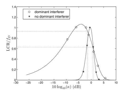
Figure 2: LCR results for the dominant and no dominant interferer cases in a Rayleigh fading scenario. The solid lines represent analytical results. Simulation values are shown by the circle and star symbols. The interference threshold values and their LCRs are shown by dotted lines.

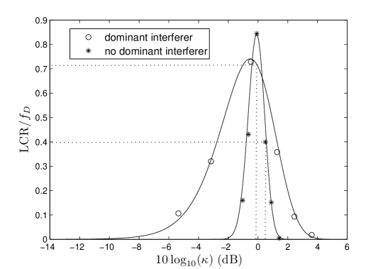
Figure 3: LCR results for the dominant and no dominant interferer cases in a Rician ($K=10$ dB) fading scenario. The solid lines represent analytical results. Simulation values are shown by the circle and star symbols. The interference threshold values and their LCRs are shown by dotted lines.

where $I_{i}$ represents the long term interference power of the $i$th CR, $h_{i}(t)$ is the corresponding normalized channel gain so that in Rayleigh fading $|h_{i}(t)|^{2}$ is a standard exponential random variable with unit mean and $N$ is the number of interfering CRs. Note that we fix the long term interference values, $I_{1},\ldots,I_{N}$ and consider the variation of the fast fading terms, $h_{i}$. From (1), the aggregate interference is represented as a weighted sum of exponential variables. Such weighted sums can be approximated by a gamma variable [7]. Simulated results show that the gamma fit is very good, but are not shown here for reasons of space. However, the corresponding LCR results are shown to be accurate in Figs. 1-3. Note that the exact LCR computation for such sums was given in [8] for the case of three and four branch maximal ratio combining (MRC) by providing special function integrals. Recently, more general expressions for arbitrary number of branches have been derived in [9]. However, the approach of [9] results in numerical difficulties, especially for large values of $N$, which can be the case for CR systems. Hence, an approximation is useful to overcome these problems and to provide a much simpler solution. Thus, approximate LCRs for (1) can be found by calculating the LCR of the equivalent gamma process. The LCR for a gamma process has been calculated in [10]. Therefore, the crossing rate of $I_{Ray}(t)$ across a threshold, $T$, can be approximated by:

$$\textrm{LCR}_{I_{Ray}}(T)=\frac{1}{2\Gamma(r)}\sqrt{\frac{2|\ddot{R}(0)|}{\pi}}(\theta T)^{r-0.5}\exp(-\theta T)$$ (2)

where $r=E(I_{Ray}(t))^{2}/Var(I_{Ray}(t))$, $\theta=E(I_{Ray}(t))/Var(I_{Ray}(t))$ and $\ddot{R}(0)=\ddot{\rho}_{Ray}(0)$ is the second derivative of the autocorrelation function (ACF) of $I_{Ray}(t)$ at time lag, $\tau=0$. Hence, to compute the LCR in (2) only the mean, variance and ACF of the random process in (1) are required. The first two moments of (1) can be computed as $E(I_{Ray}(t))=\sum_{i=1}^{N}I_{i}$ and $Var(I_{Ray}(t))=\sum_{i=1}^{N}I_{i}^{2}$. To calculate the ACF, note that:

$$h_{i}(t+\tau)=\rho_{i}(\tau)h_{i}(t)+\sqrt{(1-\rho_{i}^{2}(\tau))}e_{i}(t),$$ (3)

where $e_{i}(t)$ is independent of $h_{i}(t)$ and statistically identical to $h_{i}(t)$. Assuming a Jakes’ fading process, $\rho_{i}(\tau)$ is the zeroth order Bessel function of the first kind, $J_{0}(2\pi f_{D}\tau)$ and $f_{D}$ is the Doppler frequency. Using (3) we have:

$$E[I_{Ray}(t)I_{Ray}(t+\tau)] {}={} \sum_{i,j=1}^{N}I_{i}I_{j}E[|h_{i}(t)|^{2}|h_{j}(t+\tau)|^{2}]$$ (4)

$${}={} \sum_{i\neq j}^{N}I_{i}I_{j}+\bigg{(}\sum_{i=1}^{N}I_{i}^{2}E[|h_{i}(t)|^{2}(\rho_{i}^{2}(\tau){\times}|h_{i}(t)|^{2}+(1-\rho_{i}^{2}(\tau))|e_{i}(t)|^{2})]\bigg{)}$$

$${}={} \sum_{i\neq j}^{N}I_{i}I_{j}+\sum_{i=1}^{N}I_{i}^{2}+\sum_{i=1}^{N}I_{i}^{2}\rho_{i}^{2}(\tau)$$

$${}={} \bigg{(}\sum_{i=1}^{N}I_{i}\bigg{)}^{2}+\sum_{i=1}^{N}I_{i}^{2}\rho_{i}^{2}(\tau),$$

where in the second to last step above, we have used the fact that cross products have zero mean and that $E[|h_{i}(t)|^{4}]=2$. The ACF of (1) is given by:

$$\rho_{Ray}(\tau)\!=\!\frac{E(I_{Ray}(t)I_{Ray}(t+\tau))\!-\!E(I_{Ray}(t))E(I_{Ray}(t+\tau))}{\sqrt{Var(I_{Ray}(t))Var(I_{Ray}(t+\tau))}},$$ (5)

and with the relevant substitutions, the ACF becomes:

$$\rho_{Ray}(\tau)=\frac{\sum_{i=1}^{N}I_{i}^{2}J_{0}^{2}(2\pi f_{D}\tau)}{\sum_{i=1}^{N}I_{i}^{2}}.$$ (6)

Finally, using the expansion $J_{0}(2\pi f_{D}\tau)=1-\pi^{2}f_{D}^{2}\tau^{2}+\ldots$, the second derivative of the ACF needed to compute the LCR in (2) is evaluated as:

$$\ddot{\rho}_{Ray}(0)=-4\pi^{2}\frac{\sum_{i=1}^{N}I_{i}^{2}f_{D}^{2}}{\sum_{i=1}^{N}I_{i}^{2}}.$$ (7)

Hence, the three parameters, $r$, $\theta$ and $\ddot{R}(0)$, are available and (2) gives the approximate LCR.

II-B LCRs for Rician Fading

The instantaneous aggregate interference, $I_{Ric}(t)$, for this scenario is given as:

$$I_{Ric}(t)=\sum_{i=1}^{N}I_{i}|h_{i}(t)|^{2},$$ (8)

where $|h_{i}(t)|$ is Rician, with Rician K-factor denoted by $K$, and $N,I_{1},I_{2},\ldots,I_{N}$ are as defined in (1). Hence, $I_{Ric}(t)$ is a weighted sum of noncentral chi-square ($\chi^{2}$) random variables. Note that standard LCR results for Ricians [11, 12] and noncentral $\chi^{2}$ variables [12] cannot be applied directly here. The work in [13] is for a single Rician and in [12] the LCR applies to the case where $I_{1}=I_{2}=\ldots=I_{N}$ and an exact noncentral $\chi^{2}$ arises with integer degrees of freedom (dof). Instead, using the same approximation philosophy as that used in the Rayleigh case, we propose approximating (8) by a single noncentral $\chi^{2}$. This approach is less well documented but has appeared in the literature (see [14]). Also note that a scaled, rather than a standard, noncentral $\chi^{2}$ distribution is required for fitting and the resulting best-fitting distribution will almost certainly not have integer dof. A noncentral $\chi^{2}$ variable with $v$ dof, non-centrality parameter $\lambda$ and scale parameter $\alpha$ has the following PDF:

$$p(x)=\frac{\alpha}{2}\exp\bigg{(}\frac{-(\lambda+\alpha x)}{2}\bigg{)}\bigg{(}\frac{\alpha x}{\lambda}\bigg{)}^{\frac{v-2}{4}}I_{\frac{v-2}{2}}\big{(}\sqrt{\lambda\alpha x}\big{)},$$ (9)

where $I_{(v-2)/2}$ is a modified Bessel function of the first kind with order $(v-2)/2$. Fitting the PDF in (9) to the variable in (8) is performed using the method of moments technique so that the approximate noncentral $\chi^{2}$ has the same first three moments as $I_{Ric}(t)$. The derivation details are outlined in Appendix I. Note that there can be numerical difficulties with the approach for certain values of $I_{1},I_{2},\ldots,I_{N}$. However, when this approach does not work it is straightforward to perform a numerical minimization of the difference between the true moments of the CR interference and the moments of the $\alpha-$scaled noncentral $\chi^{2}$ variable. Values of $\lambda$, $v$ and $\alpha$ which minimize this difference can then be used.

The LCR of a noncentral $\chi^{2}$ process with integer dof can be readily obtained from [12]. In particular, if we substitute $R=T$, $\sigma^{2}=1$, $M=v/2$, $s^{2}=\lambda$ and $f_{m}=f_{D}$ in [12, Eq. (15)] we get the following expression for the LCR of the $\alpha-$scaled noncentral $\chi^{2}$ variable

$$\textrm{LCR}_{I_{Ric}} {}={} \sqrt{\pi}f_{D}(\alpha T)^{\frac{v}{4}}\lambda^{\frac{-(v-2)}{4}}e^{\big{(}\frac{-\lambda-\alpha T}{2}\big{)}}I_{\frac{v-2}{2}}\big{(}\sqrt{\lambda\alpha T}\big{)}.$$ (10)

The result in (10) holds good for a noncentral $\chi^{2}$ process with integer dof. In Appendix II we show that this formula is also valid for non-integer dof. Note that a similar extension for a central $\chi^{2}$ with integer order [15] to a central $\chi^{2}$ with fractional order [10] has also been shown to be correct.

II-C AEDs

We define the AED for both Rayleigh and Rician environments as the average time that the aggregate interference stays above a given threshold $T$ [11]. Mathematically,

$$AED=\frac{1-F(T)}{LCR}$$ (11)

where $F(T)$ gives the distribution function of the aggregate interference. Note that the exact CDFs of both $I_{Ray}(t)$ and $I_{Ric}(t)$ can be found in [16].

III Results

In order to evaluate the accuracy of (2) and (10) it is important to use realistic values of $I_{1},I_{2},\dots,I_{N}$. Hence, we use a particular CR access scheme [4] to provide these values. The decentralized selection algorithm in [4] employs a controller that considers CRs in their order of arrival. Each interferer is considered in turn and is accepted if the combined interference from previously accepted CRs and the current CR is less than some interference threshold. If a CR is not accepted, the next CR in the list is investigated. The $I_{i}$ values are generated in [4] from randomly located CRs in a circular region and include path loss and shadowing effects. In [4] a threshold value is used which corresponds to the PU accepting a $2$ dB loss in its SNR due to the presence of CRs.

From 1000 simulations, using the above selection procedure two sets of interferers were selected. The first set selected had the highest variance. Only 3 CRs were accepted and there was a dominant interferer which accounted for 95% of the interference power. The second set had the lowest variance, representing the no dominant interferer scenario. Here, 18 CRs were accepted with the largest interferer only accounting for 16%. In addition to giving examples of engineering importance (presence or absence of a dominant interferer) these two cases also test the general applicability of (2) and (10) over a wide range of interferer profiles. These sets were obtained using the following parameter values: shadow fading variance, $\sigma=8.0$ dB, path loss exponent, $\gamma=3.5$, radius of PU coverage area, $R=1000$ m, radius of CR coverage area, $R_{c}=100$ m, CR density of 1000 CRs per square kilometer, an activity factor of $0.1$ and $f_{D}=25$ Hz.

LCR and AED of CR-PU Interference

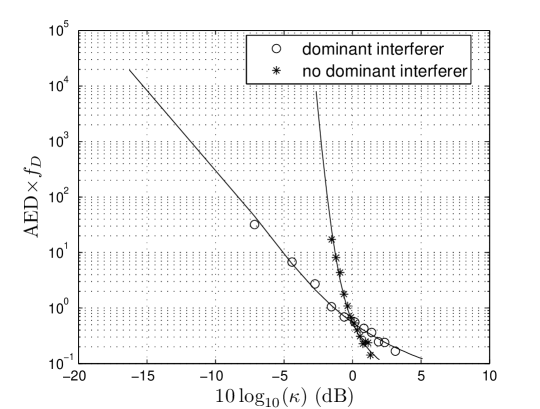
Figure 4: AED results for the dominant and no dominant interferer cases in a Rician ($K=10$ dB) fading scenario. The solid lines represent analytical results. Simulation values are shown by the circle and star symbols.

Figures 1, 2 and 3 show the LCR (normalized by Doppler frequency) of the interference for different types of fading and interference profiles. The $x$-axis is also normalized by the rms value of the process so that $\kappa=T/\sqrt{m_{2}}$ is plotted, where $T$ is the interference power level and $m_{2}$ is the mean-square interference (see Appendix I). Figure 1 shows the effect on LCR of increasing the Rician $K$-factor, with the strong LOS case being considerably narrower than the non-LOS case. Figures 2 and 3 also show the value of the normalized interference threshold that restricts the long term average interference value in the CR system (as shown by the dotted lines). Note that there are multiple thresholds since the normalization is different for different channels. For all types of fading, the maximum LCR is observed close to this threshold value. This is because the CR allocation method gives a mean interference level close to the threshold. Even in strong LOS conditions ($K=10$ dB), the interference shows a significant number of level crossings across the buffer due to the scattered component. Figure 2 shows the case of Rayleigh fading where the interference budget is dominated by a single large interferer with a number of smaller additional interferers. Also shown is the no dominant interferer case. Figure 3 shows the same results for a Rician channel with $K=10$ dB. Figures 2 and 3 show that when there are many small interferers, the interference is more stable compared to the dominant interferer case. The results in Fig. 3 are quite promising. In near LOS conditions, the interference has a much lower level crossing rate across the interference buffer for the no dominant interferer case. Hence, it may be a desirable part of the CR allocation policy to avoid any single user which takes up a significant part of the buffer. Finally, for completeness, we show the AED results corresponding to Fig. 3 in Fig. 4. As expected, the time spent by the interference above a threshold decreases as the threshold value increases. Therefore, for the no dominant interferer case, the interference seldom crosses the threshold (see Fig. 3), and when it does, it only exceeds the threshold for a small period of time. Finally, we note that all figures show an excellent agreement between the analytical approximations and the simulations.

IV Conclusion

In this paper we determine the LCR and AED for the CR-PU interference for Rayleigh and Rician channels. We have shown that LCRs in Rayleigh environment can be accurately approximated by LCRs of a gamma process. Similarly, while deriving LCR approximations in Rician conditions we have shown that the LCR of a noncentral $\chi^{2}$ process with non-integer dof has the same form as that of a noncentral $\chi^{2}$ process with integer dof. The LCR results show that it is desirable for the interference to be made up of several small interfering CRs rather than a dominant source of interference. The LCR of the former case is more stable than the latter. The AED results also show that the interference exceeds the threshold value for small periods of time in the latter case.

Appendix A

Let $Y$ denote the random variable defined by (9). The first three moments of $Y$ are [7]:

$$E(Y)={\alpha^{-1}}{(\lambda+\nu)}$$ (12)

$$E(Y^{2})={\alpha^{-2}}{((\lambda+\nu)^{2}+2(\lambda+\nu)+2\lambda)}$$ (13)

$$E(Y^{3})={\alpha^{-3}}({(\lambda+\nu)^{3}+6(\lambda+\nu)^{2}+2\lambda(\lambda+\nu)+8(\lambda+\nu)+16\lambda}).$$ (14)

Similarly, suppose $m_{1},m_{2}$ and $m_{3}$ denote the moments of $I_{Ric}(t)$ in (8) about origin. Expanding $I_{Ric}(t)$, $I_{Ric}^{2}(t)$ and $I_{Ric}^{3}(t)$ into multiple sums and taking expectation using standard results in [7] leads to:

$$m_{1}=\sum_{i=1}^{N}I_{i}$$ (15)

$$m_{2}=\bigg{(}\sum_{i=1}^{N}I_{i}\bigg{)}^{2}+\sum_{i=1}^{N}I_{i}^{2}\bigg{(}1-\bigg{(}\frac{K}{K+1}\bigg{)}^{2}\bigg{)}$$ (16)

$$m_{3}=\bigg{(}\sum_{i=1}^{N}I_{i}\bigg{)}^{3}+3\sum_{i=1}^{N}\sum_{k\neq i,k=1}^{N}I_{i}^{2}I_{k}\bigg{(}1-\bigg{(}\frac{K}{K+1}\bigg{)}^{2}\bigg{)}+\sum_{i=1}^{N}I_{i}^{3}\bigg{(}2-6\bigg{(}\frac{K}{K+1}\bigg{)}^{2}+4\bigg{(}\frac{K}{K+1}\bigg{)}^{4}\bigg{)}.$$ (17)

Now applying the method of moments, we solve $m_{k}=E(Y^{k})$ for $k=1,2,3$ and obtain the following:

$$\lambda=0.5\alpha(\alpha m_{2}-\alpha m_{1}^{2}-2m_{1}),\quad\nu=\alpha m_{1}-\lambda,$$ (18)

where $\alpha$ is the solution to the following quadratic equation:

$$\alpha^{2}m_{1}^{3}-\alpha^{2}m_{3}+6\alpha m_{1}^{2}+3\alpha^{2}m_{1}m_{2}-3\alpha^{2}m_{1}^{3}+8\alpha m_{2}-8\alpha m_{1}^{2}-8m_{1}=0.$$ (19)

Appendix B

In [12] a noncentral $\chi^{2}$ process, denoted $r$ is considered. The only part of the derivation in [12] that requires integer dof is the proof that the conditional distribution of $\dot{r}$ given $r$ is Gaussian with variance $Var(\dot{r}|r)=4\tilde{\sigma}^{2}r$ where $\tilde{\sigma}^{2}$ is a variance parameter. In this Appendix we show that this is true for a general noncentral $\chi^{2}$ process. The LCR of a stationary gamma process was first derived by Barakat [10] in an optics context building on previous results in [17]. This analysis is based on the representation [10]

$$\Omega=\int_{A}|E(x)|^{2}dx$$ (20)

where $A$ is the region of integration (an aperture in [10]), $E(x)$ is a circular complex zero-mean Gaussian process and $\Omega$ is the resulting gamma variable. If $E(x)$ is allowed to have a constant non-zero mean then for certain $A$, the resulting $\Omega$ has a scaled noncentral $\chi^{2}$ distribution with arbitrary degrees of freedom (not necessarily integer). For this noncentral case let $E(x)=E_{1}(x)+jE_{2}(x)$ and

$$\Omega=\int_{A}E_{1}^{2}(x)+E_{2}^{2}(x)dx,$$ (21)

where $E_{1}(x)$ and $E_{2}(x)$ are both non-zero mean Gaussian processes. The derivative of $\Omega$ is therefore

$$\dot{\Omega}=\int_{A}[2E_{1}(x)\dot{E_{1}}(x)+2E_{2}(x)\dot{E_{2}}(x)]dx.$$ (22)

Now it is well known [18, 12, 9, 8, 13] that $\dot{E_{1}}(x)$, $\dot{E_{2}}(x)$ are zero-mean Gaussian variables which are independent of $E_{1}(x)$, $E_{2}(x)$ and each other. Let the distribution of both derivatives be denoted by $\mathcal{N}(0,\sigma^{2})$. Hence, conditioned on $E_{1}(x)$ and $E_{2}(x)$ over $x\in A$, the derivative, $\dot{\Omega}$, is also zero mean Gaussian. The variance of $\dot{\Omega}$ conditioned on $\{E_{1}(x),E_{2}(x)|x\in A\}$ is given by

$${}E{} \bigg{[}\int_{A}\int_{A}(2E_{1}(x)\dot{E_{1}}(x)+2E_{2}(x)\dot{E_{2}}(x))(2E_{1}(y)\dot{E_{1}}(y)+2E_{2}(y)\dot{E_{2}}(y))dxdy\bigg{]}$$ (23)

$${}={} E\bigg{[}\int_{A}\big{(}4E_{1}^{2}(x)\dot{E_{1}^{2}}(x)+4E_{2}^{2}(x)\dot{E_{2}^{2}}(x)\big{)}dx\bigg{]}$$

since $\dot{E_{i}}(x)$ is independent of $\dot{E_{i}}(y)$ for $x\neq y$. Also, since $E[\dot{E_{i}}^{2}(x)]=\sigma^{2}$, the conditional variance is

$$4\sigma^{2}\int_{A}[E_{1}^{2}(x)+E_{2}^{2}(x)]dx=4\sigma^{2}\Omega$$ (24)

Hence, $\dot{\Omega}$ has the representation $\dot{\Omega}=2\sigma\Omega^{1/2}Z$ where $Z\sim\mathcal{N}(0,1)$ and $\dot{\Omega}$ has the conditional density

$$f_{\dot{\Omega}|\Omega}=\frac{\exp(\frac{-x^{2}}{8\sigma^{2}\Omega})}{\sqrt{8\pi\sigma^{2}\Omega}}.$$ (25)

Since $\dot{\Omega}\sim\mathcal{N}(0,4\sigma^{2}\Omega)$, conditional on $\Omega$, the proof is complete.

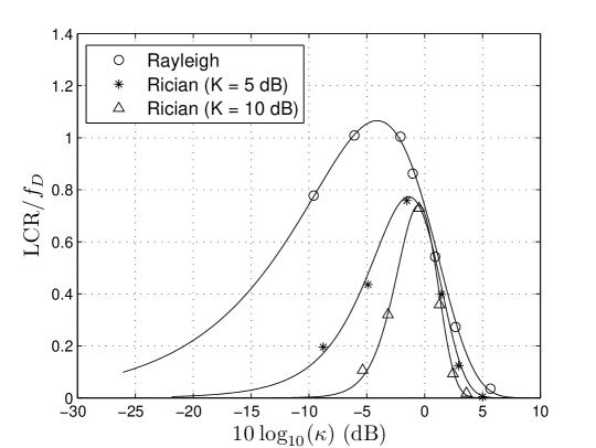
Figure 1: LCR results for different fading conditions with dominant interferers. The solid lines represent analytical results. Simulation values are shown by the circle, star and triangle symbols.

References

- [1] M. F. Hanif, P. J. Smith, and M. Shafi, “Performance of cognitive radio systems with imperfect radio environment map information,” in Proc. IEEE AusCTW, Feb. 2009, pp. 61–66.
- [2] “Spectrum Policy Task Force Report (ET Docket-135),” Federal Communications Comsssion, Tech. Rep., 2002. [Online]. Available: http://hraunfoss.fcc.gov/edocs˙public/attachmatch/DOC-228542A1.pdf
- [3] M. A. McHenry, “NSF Spectrum Occupancy Measurements Project Summary,” Shared Spectrum Company, Tech. Rep., 2005.
- [4] M. F. Hanif, M. Shafi, P. J. Smith, and P. Dmochowski, “Interference and deployment issues for cognitive radio systems in shadowing environments,” to appear in Proc. IEEE ICC, June 2009.
- [5] Y. Zhao, D. Raymond, C. da Silva, J. H. Reed, and S. F. Midkiff, “Performance evaluation of radio environment map-enabled cognitive spectrum-sharing networks,” in Proc. IEEE Military Communications Conference (MILCOM), Oct. 2007, pp. 1–7.
- [6] Y. Zhao, L. Morales, J. Gaeddert, K. K. Bae, J.-S. Um, and J. H. Reed, “Applying radio environment maps to cognitive wireless regional area networks,” in Proc. IEEE International Symposium on New Frontiers in Dynamic Spectrum Access Networks (DySPAN), April 2007, pp. 115–118.
- [7] N. L. Johnson, S. Kutz, and N. Balakrishnan, Continuous Univariate Distributions, vol. 1, 2nd ed. New York: Wiley, 1995.
- [8] X. Dong and N. C. Beaulieu, “Average level crossing rate and average fade duration of low-order maximal ratio diversity with unbalanced channels,” IEEE Communications Letters, vol. 6, no. 4, pp. 135–137, July 2002.
- [9] P. Ivanis, D. Drajic, and B. Vucetic, “The second order statistics of maximal ratio combining with unbalanced branches,” IEEE Communications Letters, vol. 12, no. 7, pp. 508–510, July 2008.
- [10] R. Barakat, “Level-crossing statistics of aperture-integrated isotropic speckle,” J. Opt. Soc. Amer., vol. 5, pp. 1244–1247, 1988.
- [11] G. L. Stuber, Principles of Mobile Communication, 2nd ed. Boston: Kluwer Academic, 2001.
- [12] N. C. Beaulieu and X. Dong, “Level crossing rate and average fade duration of MRC and EGC diversity in Ricean fading,” IEEE Trans. on Communications, vol. 51, pp. 722–726, May 2003.
- [13] M. Patzold, U. Killat, and F. Laue, “An extended Suzuki model for land mobile satellite channels and its statistical properties,” IEEE Transactions on Vehicular Technology, vol. 47, no. 2, pp. 617–630, May 1998.
- [14] H.-Y. Kim, M. J. Gribbin, K. E. Muller, and D. J. Taylor, “Analytic, computational, and approximate forms for ratios of noncentral and central gaussian quadratic forms,” Journal of Computational and Graphical Statistics, vol. 15, pp. 443–459, June 2006.
- [15] R. A. Silverman, “The fluctuation rate of the chi process,” IRE Trans. Inform. Theory, vol. 4, no. 1, pp. 30–34, Mar. 1958.
- [16] N. L. Johnson and S. Kutz, Continuous Univariate Distributions, vol. 2, 1st ed. New York: John Wiley & Sons, 1973.
- [17] R. Barakat, “Second-order statistics of integrated intensities and of detected photoelectrons,” J. Mod. Opt., vol. 34, pp. 91–102, 1987.
- [18] S. O. Rice, “Statistical properties of a sine wave plus random noise,” Bell Syst. Tech. J., vol. 27, pp. 109–157, Jan. 1948.