Evolution of squeezed states under the Fock-Darwin Hamiltonian

Abstract

We develop a complete analytical description of the time evolution of squeezed states of a charged particle under the Fock-Darwin Hamiltonian and a time-dependent electric field. This result generalises a relation obtained by Infeld and Plebański for states of the one-dimensional harmonic oscillator. We relate the evolution of a state-vector subjected to squeezing to that of state which is not subjected to squeezing and for which the time-evolution under the simple harmonic oscillator dynamics is known (e.g. an eigenstate of the Hamiltonian). A corresponding relation is also established for the Wigner functions of the states, in view of their utility in the analysis of cold-ion experiments. In an appendix, we compute the response functions of the FD Hamiltonian to an external electric field, using the same techniques as in the main text.

I Introduction

The study of the time-evolution of a non-relativistic charged particle in homogeneous magnetic and electric fields has a long history in physics. In a quantum context, the treatment of the problem goes back to Darwin Darwin27 , who considered the evolution of a Gaussian wave-packet in a magnetic field, and Fock Fock28 who obtained the eigenenergies and eigenstates of a charged particle in an isotropic harmonic potential, subjected to a magnetic field normal to the plane of motion.

If one takes a particle of charge $-e$ and mass $m$, moving in the $xy$ plane in an harmonic potencial of frequency $\omega_{0}$ and subjected to a magnetic field $\mbox{${\bm{B}}$}=B\mbox{${\bm{e}}$}_{z}$, the Hamiltonian describing the system is given, in the symmetric gauge where $\mbox{${\bm{A}}$}=\frac{1}{2}\,\mbox{${\bm{B}}$}\times\mbox{${\bm{r}}$}$, by

$$\hat{H}_{0}=\frac{1}{2m}\,\left[\left(\hat{p}_{x}-\frac{eB}{2}\hat{y}\right)^{2}+\left(\hat{p}_{y}+\frac{eB}{2}\hat{x}\right)^{2}\right]+\frac{1}{2}\,m\,\omega_{0}^{2}\,(\hat{x}^{2}+\hat{y}^{2})\,,$$ (1)

where the operators $\hat{x},\hat{p}_{x},\hat{y},\hat{p}_{y}$ obey the canonical commutation relations.

This simple problem has applications in the context of the Quantum Hall effect Hajdu94 , where disorder and the Coulomb interaction also play a crucial role. Another field for which the study of this Hamiltonian has proved fruitful is that of quantum dots, where the simple Hamiltonian given by (1) seems to give a good account of the $I-V_{g}$ curves obtained when a gate voltage is applied to the quantum dot Kouwenhoven01 , with corrections due to the assymetry of the confining potential and to the Coulomb interactions also playing a role. For some types of quantum dots, such as InAs/GaAs quantum dots, the agreement between the theoretical and experimental results seems to hold for magnetic fields up to 15 T Babinski06 .

The study of the evolution of Gaussian wave packets also goes back to the first days of quantum mechanics. This study was first undertaken by Schrödinger Schrodinger26 , Kennard Kennard27 and also by Darwin Darwin27 in the context of the harmonic oscillator, of a free particle and of a particle in constant electric and magnetic fields. This problem continues to attract attention to the present day in many contexts, see the review by Dodonov Dodonov02 .

Schrödinger considered the time-evolution of a minimal uncertainty state, i.e. a coherent state of the harmonic oscillator, in the terminology of Glauber Glauber63 . These states have a wide range of applications in quantum optics (see e.g. Leonhardt97 ), where they act as the quasi-classical states of the EM field, and in quantum field theory, where they are the basis of the phase-space path integral Brown94 . Such states and their derivatives have become important in quantum information processing in recent years, in the context of the manipulation of cold atoms in traps. It has become possible to reconstruct the Wigner function of a coherent state of the center-of-mass of an harmonically bound ion Leibfried96 .

Kennard has on the other hand considered the evolution of a more general wavepacket of the harmonic oscillator, what is now known as a squeezed state. Important early contributions are those of Husimi Husimi53 and Infeld and Plebański Infeld55 ; Plebanski56 . These later authors introduced the so-called squeezing operator and established a relation between the evolution of initial states for which the time-evolution is known (’unsqueezed states’) and states which are derived from such initial states by the application of the squeezing operator (’squeezed states’). The generalisation of this relation to the FD Hamiltonian in an homogeneous time-dependent electric field is the main result of the present paper. Stoler Stoler70 ; Stoler71 proved that squeezed-coherent states are unitarily equivalent to coherent states, thus being minimal uncertainty states, but that their minimal character is not preserved by time-evolution, although the uncertainty periodically assumes the minimum value compatible with Heisenberg’s uncertainty relation. He also showed that the squeezing operator as currently written in terms of quadratures operators is exactly of the form given by Infeld and Plebański. Squeezed states play a proeminent role in quantum optics, see again Leonhardt97 . Recently, they have also become important in quantum information processing both in a quantum optics context and also through the manipulation of cold atoms Heinzen90 ; Cirac93 ; Zeng95 ; Meekhof96 ; Ban99 ; Braunstein00 ; Braunstein05 ; Vahlbruch07 ; Polzik08 ; Adesso08 . See in particular reference Kimble08 for an up-to-date report of the state of quantum information processing using cold atoms and photons.

Besides the paper of Darwin already referred, the time-evolution of states of a non-relativistic particle in homogeneous electric and magnetic fields was also considered by Malkin, Man’ko, Trifonov and Dodonov Malkin69 ; Malkin69a ; Malkin70 ; Malkin70a ; Dodonov72 , who considered the dynamics of a particle in an homogeneous electromagnetic field in terms of coherent states, obtaining an explicit representation of the Green’s function, and studied the invariants of the system; by Lewis and Riesenfeld Lewis69 , who also considered the invariants of such a system; by Kim and Weiner Kim73 , who considered the evolution of Gaussian wave-packets in a magnetic field, subjected to an isotropic harmonic potential (i.e. the FD Hamiltonian), but also to sadle-point potentials, which are relevant for tunnelling problems.

The structure of this paper is as follows: in the next section, we review the notion of squeezing operator and generalise the relation of Infeld and Plebański to states evolving under the Fock-Darwin Hamiltonian. In section III, with a view to applications in the manipulation of cold atoms, we use the relation obtained to establish a relation between the Wigner function of different states and apply it to the special case of squeezed-coherent states. In section IV, we present our conclusions. In appendix A, we present a derivation of the finite frequency permitivity and conductivity of the FD Hamiltonian that uses the same operator methods that are used in the main text but which lies somewhat outside of the scope of the main text. Finally, in appendix B, we derive the original Infeld-Plebański relation through elementary means.

II Evolution of squeezed states under the FD Hamiltonian

We consider the time-evolution of the state $\mid\overline{\psi}_{t}\,\rangle$, that obeys the time-dependent Schrödinger equation $i\hbar\,\partial_{t}\,\mbox{$\mid\overline{\psi}_{t}\,\rangle$}=\hat{H}(t)\,\mbox{$\mid\overline{\psi}_{t}\,\rangle$}$, where $\hat{H}(t)=\hat{H}_{0}+\hat{H}_{1}(t)$, with $\hat{H}_{0}$ being given by equation (1) and where the interaction Hamiltonean $\hat{H}_{1}(t)$ of the charge with the external electric field is given, in the Schrödinger picture, by $\hat{H}_{1}(t)=e(E_{x}(t)\hat{x}+E_{y}(t)\hat{y})$.

If one now expands the squares and groups the different terms of (1), one obtains

$$\hat{H}_{0}=\frac{1}{2m}\,\left(\hat{p}_{x}^{2}+\hat{p}_{y}^{2}\right)+\frac{1}{2}\,m\,\omega_{R}^{2}\,(\hat{x}^{2}+\hat{y}^{2})+\frac{\omega_{L}}{2}\,\hat{L}_{z}\,,$$ (2)

where $\omega_{L}=\frac{eB}{m}$ is the giration frequency and $\omega_{R}^{2}=\omega_{0}^{2}+\frac{\omega_{L}^{2}}{4}$, with $\hat{L}_{z}=\hat{x}\hat{p}_{y}-\hat{y}\hat{p}_{x}$ being the angular momentum component along the $z$ axis. One should note that one can write $\hat{H}_{0}=\hat{h}_{0}+\frac{\omega_{L}}{2}\,\hat{L}_{z}$, where $\hat{h}_{0}$ is the Hamiltonean of the isotropic harmonic oscillator with frequency $\omega_{R}$, and also that $[\hat{h}_{0},\hat{L}_{z}]=0$.

Given the state vector $\mid\overline{\psi}_{t}\,\rangle$, one can define the corresponding state vector $\mbox{$\mid\phi_{t}\,\rangle$}=e^{\frac{i}{\hbar}\,\hat{H}_{0}t}\,\mbox{$\mid\overline{\psi}_{t}\,\rangle$}$, in the interaction representation, such that the two vectors coincide at $t=0$. This state vector evolves acording to the Hamiltonian $\hat{H}_{1}^{int}(t)=e^{\frac{i}{\hbar}\,H_{0}t}\,\hat{H}_{1}(t)\,e^{-\frac{i}{\hbar}\,H_{0}t}$, which given that $\hat{h}_{0}$ and $\hat{L}_{z}$ in $\hat{H}_{0}$ commute, one can also write as

$$\hat{H}_{1}^{int}(t)=e^{\frac{i}{\hbar}\,\hat{h}_{0}t}\,e^{\frac{i\omega_{L}t}{2\hbar}\,\hat{L}_{z}}\,\hat{H}_{1}(t)\,e^{-\frac{i\omega_{L}t}{2\hbar}\,\hat{L}_{z}}\,e^{-\frac{i}{\hbar}\,\hat{h}_{0}t}\,.$$ (3)

If one now applies the time-dependent rotation, encoded by $\hat{L}_{z}$ to $\hat{H}_{1}(t)$, followed by the dynamics of the isotropic harmonic oscillator, encoded in $\hat{h}_{0}$, one obtains for $\hat{H}_{1}^{int}(t)$:

$$\hat{H}_{1}^{int}(t) = e\left\{E_{x}^{\prime}(t)\left[\,\hat{x}\,\cos(\omega_{R}t)+\hat{p}_{x}\,\sin(\omega_{R}t)\,\right]+\,E_{y}^{\prime}(t)\left[\,\hat{y}\,\cos(\omega_{R}t)+\hat{p}_{y}\,\sin(\omega_{R}t)\,\right]\right\},$$ (4)

where

$$E_{x}^{\prime}(t) = E_{x}(t)\cos\left(\frac{\omega_{L}}{2}\,t\right)+E_{y}(t)\sin\left(\frac{\omega_{L}}{2}\,t\right)\,,$$ (5)

$$E_{y}^{\prime}(t) = -E_{x}(t)\sin\left(\frac{\omega_{L}}{2}\,t\right)+E_{y}(t)\cos\left(\frac{\omega_{L}}{2}\,t\right)\,,$$ (6)

are the components of the electric field in the rotated frame.

The wave equation for $\mid\phi_{t}\,\rangle$ can be formally integrated in terms of time-ordered products of the integral of $\hat{H}_{1}^{int}(t)$, i.e. $\mbox{$\mid\phi_{t}\,\rangle$}=T\,\exp\left(-\frac{i}{\hbar}\,\int_{0}^{t}\,du\,\hat{H}_{1}^{int}(u)\right)\,\mbox{$\mid\overline{\psi}_{0}\,\rangle$}$. Now, since the commutator of the operators $\hat{H}_{1}^{int}(u)$ at different times is a c-number, one can write the time ordered operator above as

$$T\,\exp\left(-\frac{i}{\hbar}\,\int_{0}^{t}\,du\,\hat{H}_{1}^{int}(u)\right) = \exp\left(-\frac{i}{\hbar}\,\int_{0}^{t}\,du\,\hat{H}_{1}^{int}(u)\right)$$ (7)

$$\mbox{}\times\,\exp\left(-\frac{1}{2\hbar^{2}}\,\int_{0}^{t}\,du\,\int_{0}^{u}\,dv\,[\hat{H}_{1}^{int}(u),\hat{H}_{1}^{int}(v)]\right)\,,$$

where the second term on the rhs is a phase factor.

Collecting the several terms, one obtains for the evolution of $\mid\overline{\psi}_{t}\,\rangle$

$$\mid\overline{\psi}_{t}\,\rangle = \exp\left(\frac{ie^{2}}{2\hbar m\omega_{R}}\,\int_{0}^{t}\,du\,\int_{0}^{u}\,dv\,\sin[\,\omega_{R}(u-v)\,]\,\,[E_{x}^{\prime}(u)E_{x}^{\prime}(v)+E_{y}^{\prime}(u)E_{y}^{\prime}(v)]\right)$$ (8)

$$\mbox{}\times\exp\left(-\frac{i\omega_{L}t}{2\hbar}\,\hat{L}_{z}\right)\,\exp\left(-\frac{i}{\hbar}\,\hat{h}_{0}\,t\right)\,\exp\left(-\frac{i}{\hbar}\,\int_{0}^{t}\,du\,\hat{H}_{1}^{int}(u)\right)\,\mbox{$\mid\overline{\psi}_{0}\,\rangle$}\,.$$

One now assumes, following Infeld and Plebański Plebanski56 , that the initial state $\mid\overline{\psi}_{0}\,\rangle$ is related to a certain initial state $\mid\psi_{0}\,\rangle$, for which the time-evolution under the isotropic harmonic oscillator Hamiltonian $\hat{h}_{0}$ is known, by

$$\mbox{$\mid\overline{\psi}_{0}\,\rangle$}=\exp\left(\frac{i}{\hbar}(\,P^{0}_{x}\hat{x}+P^{0}_{y}\hat{y}-X_{0}\hat{p}_{x}-Y_{0}\hat{p}_{y}\,)\right)\,\exp\left(\frac{i}{2\hbar}\,r\,(\hat{\mbox{${\bm{p}}$}}\cdot\hat{\mbox{${\bm{r}}$}}+\hat{\mbox{${\bm{r}}$}}\cdot\hat{\mbox{${\bm{p}}$}})\right)\,\mbox{$\mid\psi_{0}\,\rangle$}\,,$$ (9)

where the first operator is a translation operator in phase space, with $X_{0},Y_{0},P_{x}^{0},P_{y}^{0}$ being arbitrary real constants, and the second operator is the squeezing operator, with $r$ being a real constant that indicates the degree of squeezing.

Substituting equation (9) in (8) one can combine the operators $e^{-\frac{i}{\hbar}\,\int_{0}^{t}\,du\,\hat{H}_{1}^{int}(u)}$ and $e^{\frac{i}{\hbar}(\,P^{0}_{x}\hat{x}+P^{0}_{y}\hat{y}-X_{0}\hat{p}_{x}-Y_{0}\hat{p}_{y}\,)}$, since the commutator of their exponents is a c-number. This operation merely generates a phase factor, coming from the commutator. One can then commute the resulting operator to the left-hand side, through $e^{-\frac{i\omega_{L}t}{2\hbar}\,\hat{L}_{z}}\,e^{-\frac{i}{\hbar}\,\hat{h}_{0}t}$, using the time-evolution of $\hat{x},\hat{p}_{x},\hat{y},\hat{p}_{y}$ under $\hat{h}_{0}$ and under the time-dependent rotation around the $z$ axis. Combining the resulting phase factors and operators, we obtain

$$\mid\overline{\psi}_{t}\,\rangle = \exp\left(-\frac{ie}{2\hbar}\,\int_{0}^{t}\,du\,\,[E_{x}(u)\,x_{c}(u)+E_{y}(u)\,y_{c}(u)]\right)\,\exp\left(\frac{i}{\hbar}(\,p^{c}_{x}(t)\hat{x}+p^{c}_{y}(t)\hat{y}-x_{c}(t)\hat{p}_{x}-y_{c}(t)\hat{p}_{y}\,)\right)$$ (10)

$$\mbox{}\times\exp\left(-\frac{i\omega_{L}t}{2\hbar}\,\hat{L}_{z}\right)\,\exp\left(-\frac{i}{\hbar}\,\hat{h}_{0}\,t\right)\,\exp\left(\frac{i}{2\hbar}\,r\,(\hat{\mbox{${\bm{p}}$}}\cdot\hat{\mbox{${\bm{r}}$}}+\hat{\mbox{${\bm{r}}$}}\cdot\hat{\mbox{${\bm{p}}$}})\right)\,\mbox{$\mid\psi_{0}\,\rangle$}\,.$$

where $x_{c}(t)$, $y_{c}(t)$, $p_{x}^{c}(t)$ and $p_{y}^{c}(t)$ are the classical solutions of the equations of motion for the Fock-Darwin problem with initial positions $X_{0}$ and $Y_{0}$ and initial momenta $P_{x}^{0}$ and $P_{y}^{0}$. These solutions are given by

$$x_{c}(t) = \left[\,X_{0}\cos\left(\frac{\omega_{L}}{2}t\right)-Y_{0}\sin\left(\frac{\omega_{L}}{2}t\right)\,\right]\,\cos(\omega_{R}t)$$ (11)

$$\mbox{}+\frac{1}{m\omega_{R}}\,\left[\,P_{x}^{0}\cos\left(\frac{\omega_{L}}{2}t\right)-P_{y}^{0}\sin\left(\frac{\omega_{L}}{2}t\right)\,\right]\,\sin(\omega_{R}t)$$

$$\mbox{}-\frac{e}{2m\omega_{R}}\,\int_{0}^{t}\,du\,\left\{E_{x}(u)\,\left[\sin(\omega_{+}(t-u))+\sin(\omega_{-}(t-u))\right]\right.$$

$$\mbox{}\left.+E_{y}(u)\,\left[\cos(\omega_{+}(t-u))-\cos(\omega_{-}(t-u))\right]\right\}\,,$$

$$y_{c}(t) = \left[\,X_{0}\sin\left(\frac{\omega_{L}}{2}t\right)+Y_{0}\cos\left(\frac{\omega_{L}}{2}t\right)\,\right]\,\cos(\omega_{R}t)$$ (12)

$$\mbox{}+\frac{1}{m\omega_{R}}\,\left[\,P_{x}^{0}\sin\left(\frac{\omega_{L}}{2}t\right)+P_{y}^{0}\cos\left(\frac{\omega_{L}}{2}t\right)\,\right]\,\sin(\omega_{R}t)$$

$$\mbox{}-\frac{e}{2m\omega_{R}}\,\int_{0}^{t}\,du\,\left\{-E_{x}(u)\,\left[\cos(\omega_{+}(t-u))-\cos(\omega_{-}(t-u))\right]\right.$$

$$\mbox{}\left.+E_{y}(u)\,\left[\sin(\omega_{+}(t-u))+\sin(\omega_{-}(t-u))\right]\right\}\,,$$

and

$$p_{x}^{c}(t) = \left[\,P_{x}^{0}\cos\left(\frac{\omega_{L}}{2}t\right)-P_{y}^{0}\sin\left(\frac{\omega_{L}}{2}t\right)\,\right]\,\cos(\omega_{R}t)$$ (13)

$$\mbox{}-m\omega_{R}\,\left[\,X_{0}\cos\left(\frac{\omega_{L}}{2}t\right)-Y_{0}\sin\left(\frac{\omega_{L}}{2}t\right)\,\right]\,\sin(\omega_{R}t)$$

$$\mbox{}-\frac{e}{2}\,\int_{0}^{t}\,du\,\left\{E_{x}(u)\,\left[\cos(\omega_{+}(t-u))+\cos(\omega_{-}(t-u))\right]\right.$$

$$\mbox{}\left.-E_{y}(u)\,\left[\sin(\omega_{+}(t-u))-\sin(\omega_{-}(t-u))\right]\right\}\,,$$

$$p_{y}^{c}(t) = \left[\,P_{x}^{0}\sin\left(\frac{\omega_{L}}{2}t\right)+P_{y}^{0}\cos\left(\frac{\omega_{L}}{2}t\right)\,\right]\,\cos(\omega_{R}t)$$ (14)

$$\mbox{}-m\omega_{R}\,\left[\,X_{0}\sin\left(\frac{\omega_{L}}{2}t\right)+Y_{0}\cos\left(\frac{\omega_{L}}{2}t\right)\,\right]\,\sin(\omega_{R}t)$$

$$\mbox{}-\frac{e}{2}\,\int_{0}^{t}\,du\,\left\{E_{x}(u)\,\left[\sin(\omega_{+}(t-u))-\sin(\omega_{-}(t-u))\right]\right.$$

$$\mbox{}\left.+E_{y}(u)\,\left[\cos(\omega_{+}(t-u))+\cos(\omega_{-}(t-u))\right]\right\}\,.$$

One can read the classical dielectric permitivity of the system from equations (11,12) and one obtains the same results as in appendix A, which shows that the quantum and classical results are identical, as one would expect for a linear system. The classical velocities $v_{x}^{c}(t),v_{y}^{c}(t)$ can be easily computed by derivation of (11,12) with respect to time or, using the relations $v_{x}^{c}(t)=\frac{1}{m}\left(p_{x}^{c}(t)-\frac{eB}{2}\,y_{c}(t)\right)$ and $v_{y}^{c}(t)=\frac{1}{m}\left(p_{y}^{c}(t)+\frac{eB}{2}\,x_{c}(t)\right)$, from equations (11) to (14). One can then read the classical conductivity of the system from the resulting expression and this result again coincides with that of appendix A, i.e. the classical and quantum results are the same. Finally, one can also show, after derivation of the velocity expressions with respect to time, that the solution given by (11) and (12) obeys the classical equations of motion in two dimensions $\ddot{\mbox{${\bm{r}}$}}=-\frac{e}{m}(\mbox{${\bm{E}}$}(t)+\,\dot{\mbox{${\bm{r}}$}}\times\mbox{${\bm{B}}$})-\omega_{0}^{2}\,\mbox{${\bm{r}}$}$, with $\mbox{${\bm{B}}$}=B\,\mbox{${\bm{e}}$}_{z}$.

The left most operator in equation (10) is again a translation operator in phase phase. If one considers the wave-function in the coordinate representation, $\overline{\psi}(x,y,t)=\langle\,x,y\,\mbox{$\mid\overline{\psi}_{t}\,\rangle$}$, and one applies this translation operator to $\langle\,x,y\mid$, followed by the rotation operator $e^{-\frac{i\omega_{L}t}{2\hbar}\,\hat{L}_{z}}$, one obtains the following result

$$\overline{\psi}(x,y,t) = \exp\left(-\frac{i}{2\hbar}\left(\,p_{x}^{c}(t)\,x_{c}(t)+p_{y}^{c}\,y_{c}(t)+e\int_{0}^{t}\,du\,[E_{x}(u)\,x_{c}(u)+E_{y}(u)\,y_{c}(u)]\,\right)\right)$$ (15)

$$\mbox{}\times\exp\left(\frac{i}{\hbar}[p^{c}_{x}(t)\,x+p^{c}_{y}(t)\,y]\right)\,\mbox{$\langle\,{\cal R}^{-1}_{t}\cdot\,(\,\mbox{${\bm{r}}$}-\mbox{${\bm{r}}$}_{c}(t)\,)\mid$}\,\,e^{-\frac{i}{\hbar}\,\hat{h}_{0}\,t}\,e^{\frac{i}{2\hbar}\,r\,(\hat{\mbox{\bf\scriptsize p}}\cdot\hat{\mbox{\bf\scriptsize r}}+\hat{\mbox{\bf\scriptsize r}}\cdot\hat{\mbox{\bf\scriptsize p}})}\,\mbox{$\mid\psi_{0}\,\rangle$}\,,$$

with $\mbox{${\bm{r}}$}_{c}(t)$ being the classical solutions of the equations of motion (11) and (12) and ${\cal R}_{t}$ being the rotation matrix in two dimensions by an angle of $\omega_{L}t/2$.

For the wave-function in the momentum representation $\overline{\psi}(p_{x},p_{y},t)=\langle\,p_{x},p_{y}\,\mbox{$\mid\overline{\psi}_{t}\,\rangle$}$, one obtains, applying the translation operator to $\langle\,p_{x},p_{y}\mid$, followed again by the rotation operator,

$$\overline{\psi}(p_{x},p_{y},t) = \exp\left(\frac{i}{2\hbar}\left(\,p_{x}^{c}(t)\,x_{c}(t)+p_{y}^{c}\,y_{c}(t)-e\int_{0}^{t}\,du\,[E_{x}(u)\,x_{c}(u)+E_{y}(u)\,y_{c}(u)]\,\right)\right)$$ (16)

$$\mbox{}\times\exp\left(-\frac{i}{\hbar}[p_{x}\,x_{c}(t)+p_{y}\,y_{c}(t)]\right)\,\mbox{$\langle\,{\cal R}^{-1}_{t}\cdot\,(\,\mbox{${\bm{p}}$}-\mbox{${\bm{p}}$}^{c}(t)\,)\mid$}\,\,e^{-\frac{i}{\hbar}\,\hat{h}_{0}t}\,e^{\frac{i}{2\hbar}\,r\,(\hat{\mbox{\bf\scriptsize p}}\cdot\hat{\mbox{\bf\scriptsize r}}+\hat{\mbox{\bf\scriptsize r}}\cdot\hat{\mbox{\bf\scriptsize p}})}\,\mbox{$\mid\psi_{0}\,\rangle$}\,,$$

with $\mbox{${\bm{p}}$}^{c}(t)$ being the classical solutions of the equations of motion (13) and (14).

One can now apply the relation of Infeld and Plebański Plebanski56 , relating the evolution of $\mbox{$\langle\,x,y\mid$}\,\,e^{-\frac{i}{\hbar}\,\hat{h}_{0}t}\,e^{\frac{i}{2\hbar}\,r\,(\hat{\mbox{\bf\scriptsize p}}\cdot\hat{\mbox{\bf\scriptsize r}}+\hat{\mbox{\bf\scriptsize r}}\cdot\hat{\mbox{\bf\scriptsize p}})}\,\mbox{$\mid\psi_{0}\,\rangle$}$ to that of $\mbox{$\langle\,x,y\mid$}\,\,e^{-\frac{i}{\hbar}\,\hat{h}_{0}t}\,\mbox{$\mid\psi_{0}\,\rangle$}$ and the evolution of $\mbox{$\langle\,p_{x},p_{y}\mid$}\,\,e^{-\frac{i}{\hbar}\,\hat{h}_{0}t}\,e^{\frac{i}{2\hbar}\,r\,(\hat{\mbox{\bf\scriptsize p}}\cdot\hat{\mbox{\bf\scriptsize r}}+\hat{\mbox{\bf\scriptsize r}}\cdot\hat{\mbox{\bf\scriptsize p}})}\,\mbox{$\mid\psi_{0}\,\rangle$}$ to that of $\mbox{$\langle\,p_{x},p_{y}\mid$}\,\,e^{-\frac{i}{\hbar}\,\hat{h}_{0}t}\,\mbox{$\mid\psi_{0}\,\rangle$}$, to equations (15) and (16), respectively. This relation is derived by elementary means in appendix B.

One obtains for (15) the result

$$\overline{\psi}(x,y,t) = \mu_{r}^{-1}(t)\,\exp\left(-\frac{i}{2\hbar}\,\left(p_{x}^{c}(t)\,x_{c}(t)+p_{y}^{c}\,y_{c}(t)\,+\,e\int_{0}^{t}\,du\,\,[E_{x}(u)\,x_{c}(u)+E_{y}(u)\,y_{c}(u)]\right)\right)$$ (17)

$$\mbox{}\times\exp\left(\frac{i}{\hbar}(p^{c}_{x}(t)\,x+p^{c}_{y}(t)\,y)\right)\,\exp\left(\,\frac{i\,m\,\omega_{R}\,\sinh(2r)\sin(2\omega_{R}t)}{2\,\hbar\,\mu_{r}^{2}(t)}\,[\,(x-x_{c}(t))^{2}+(y-y_{c}(t))^{2}\,]\,\right)$$

$$\mbox{}\times\psi\left(\frac{{\cal R}^{-1}_{t}\cdot\,(\,\mbox{${\bm{r}}$}-\mbox{${\bm{r}}$}_{c}(t)\,)}{\mu_{r}(t)},\tau_{r}\right)\,,$$

where $\mu_{r}(t)=\sqrt{e^{-2r}\cos^{2}(\omega_{R}t)+e^{2r}\sin^{2}(\omega_{R}t)}$ and $\tau_{r}=\frac{1}{\omega_{R}}\,\arctan(e^{2r}\tan(\omega_{R}t))$.

For equation (16), one obtains

$$\overline{\psi}(p_{x},p_{y},t) = \mu_{-r}^{-1}(t)\,\exp\left(\frac{i}{2\hbar}\,\left(p_{x}^{c}(t)\,x_{c}(t)+p_{y}^{c}\,y_{c}(t)\,-\,e\int_{0}^{t}\,du\,\,[E_{x}(u)\,x_{c}(u)+E_{y}(u)\,y_{c}(u)]\right)\right)$$ (18)

$$\mbox{}\times\exp\left(-\frac{i}{\hbar}[p_{x}\,x_{c}(t)+p_{y}\,y_{c}(t)]\right)\exp\left(-\frac{i\,\sinh(2r)\sin(2\omega_{R}t)}{2\,\hbar\,m\,\omega_{R}\,\mu_{-r}^{2}(t)}\,[\,(p_{x}-p_{x}^{c}(t))^{2}+(p_{y}-p_{y}^{c}(t))^{2}\,]\right)$$

$$\mbox{}\times\psi\left(\frac{{\cal R}^{-1}_{t}\cdot\,(\,\mbox{${\bm{p}}$}-\mbox{${\bm{p}}$}^{c}(t)\,)}{\mu_{-r}(t)},\tau_{-r}\right)\,,$$

where $\mu_{-r}(t)=\sqrt{e^{2r}\cos^{2}(\omega_{R}t)+e^{-2r}\sin^{2}(\omega_{R}t)}$ and $\tau_{-r}=\frac{1}{\omega_{R}}\,\arctan(e^{-2r}\tan(\omega_{R}t))$. The expressions (17) and (18) constitute the main result of this paper and generalise those of Infeld and Plebański as presented in Plebanski56 to states evolving under the Fock-Darwin Hamiltonian subjected to a time-dependent electric field in the plane of the system.

III The Wigner function for a squeezed state

One can also establish a relation between the Wigner function of a state subjected to squeezing in the presence of electric and magnetic fields and the Wigner function of an ’unsqueezed state’ evolving under the isotropic harmonic oscillator dynamics.

The Wigner function is defined as Wigner32

$$D(\mbox{${\bm{r}}$},\mbox{${\bm{p}}$},t)=\frac{1}{(2\pi\hbar)^{2}}\,\int\,d^{2}v\,e^{-\frac{i}{\hbar}\mbox{\bf\scriptsize p}\cdot\mbox{\bf\scriptsize v}}\,\overline{\psi}^{*}(\mbox{${\bm{r}}$}-\mbox{${\bm{v}}$}/2,t)\,\overline{\psi}(\mbox{${\bm{r}}$}+\mbox{${\bm{v}}$}/2,t)\,.$$ (19)

The Wigner function gives, after integration with respect to the momentum ${\bm{p}}$ or to the coordinate ${\bm{r}}$, the coordinate or momentum distribution function of the system and can be considered a quantum generalisation of the Boltzmann distribution function. However, the Wigner function is not a bonna-fide distribution since it can assume negative values.

Substituting the result of equation (17) in (19), one obtains, after a substitution of variable on ${\bm{v}}$

$$D(\mbox{${\bm{r}}$},\mbox{${\bm{p}}$},t)=D_{0}\left(\frac{{\cal R}^{-1}_{t}\cdot[\mbox{${\bm{r}}$}-\mbox{${\bm{r}}$}_{c}(t)]}{\mu_{r}(t)},{\cal R}^{-1}_{t}\cdot\mbox{${\bm{u}}$}(\mbox{${\bm{r}}$},\mbox{${\bm{p}}$},t),\tau_{r}\right)\,,$$ (20)

where $\mbox{${\bm{u}}$}(\mbox{${\bm{r}}$},\mbox{${\bm{p}}$},t)=\mu_{r}(t)[\mbox{${\bm{p}}$}-\mbox{${\bm{p}}$}^{c}(t)]-m\omega_{R}\sinh(2r)\sin(2\omega_{R}t)\frac{\mbox{${\bm{r}}$}-\mbox{${\bm{r}}$}_{c}(t)}{\mu_{r}(t)}$ and where $D_{0}(\mbox{${\bm{r}}$},\mbox{${\bm{p}}$},t)$ is the Wigner function of the ’unsqueezed’ initial state $\psi_{0}(x,y)$ evolving under the isotropic harmonic oscillator dynamics in the absence of magnetic or electric fields.

If the ’unsqueezed’ initial state $\mid\psi_{0}\,\rangle$ in equation (9) is the vacuum of the isotropic harmonic oscillator, then the state $\mid\overline{\psi}_{0}\,\rangle$ is a squeezed-coherent state, evolving under the Fock-Darwin Hamiltonian. In the context of cold ion experiments, one can produce squeezed states of the ion center of mass, either by queenching of the trap frequency or parametric amplification Heinzen90 , as well as multichromatic excitation of the ion Cirac93 ; Zeng95 ; Meekhof96 .

In this case, $D_{0}(\mbox{${\bm{r}}$},\mbox{${\bm{p}}$},t)=\frac{1}{\pi^{2}\hbar^{2}}\,e^{-\frac{m\omega_{R}}{\hbar}\mbox{\bf\scriptsize r}^{2}-\frac{\mbox{\bf\scriptsize p}^{2}}{\hbar m\omega_{R}}}$, and we obtain for the Wigner function of the squeezed-coherent state the result

$$D(\mbox{${\bm{r}}$},\mbox{${\bm{p}}$},t)=\frac{1}{\pi^{2}\hbar^{2}}\,e^{-\frac{m\omega_{R}\mu_{-r}^{2}(t)}{\hbar}\,(\mbox{\bf\scriptsize r}-\mbox{\bf\scriptsize r}_{c}(t))^{2}-\frac{\mu_{r}^{2}(t)}{\hbar m\omega_{R}}\,(\mbox{\bf\scriptsize p}-\mbox{\bf\scriptsize p}^{c}(t))^{2}+\frac{2}{\hbar}\sinh(2r)\,\sin(2\omega_{R}t)\,(\mbox{\bf\scriptsize p}-\mbox{\bf\scriptsize p}^{c}(t))\cdot(\mbox{\bf\scriptsize r}-\mbox{\bf\scriptsize r}_{c}(t))}\,,$$ (21)

which represents an assymetric Gaussian, whose shape is preserved by the dynamics of the system, rotating in phase-space, with its center determined by the solutions of the classical equations of motion (11-14). Note that for $r=0$, i.e. for a coherent state, the Wigner function decouples into a product of functions that depend only on the coordinates or the momenta. Also, note that for the result (21) is strictly positive, but this is not the case in general, e.g. if we had taken $\mid\psi_{0}\,\rangle$ to be an excited-state of the harmonic oscillator.

A group of still pictures of the $x,p_{x}$ section of the Wigner function (21) is shown in the figures, for a system subjected to a right-handed circularly polarised wave, incident along the $zz$ axis and aligned with the $xx$ axis at $t=0$. The intensity of the field is $E_{0}=100$ Vm^-1, with frequency equal to $\Omega=1.42\times 10^{9}$ Hz. The harmonic frequency of the trap is $\omega_{0}=7.04\times 10^{7}$ Hz and the mass of the particle $m=1.50\times 10^{-26}$ Kg, is that of a ${}^{9}Be^{+}$ ion, with the applied magnetic field being $B=6.60$ T, which gives a giration frequency $\omega_{L}=7.06\times 10^{7}$ Hz and $\omega_{R}=7.88\times 10^{7}$ Hz. Finally, the squeezing parameter $r=0.35$.

The integration of expression (21) with respect to ${\bm{p}}$ or ${\bm{r}}$ yields the coordinate or momentum distribution. The wave-packets in coordinate or position space are centered around the classical solutions of the equations of motion, the uncertainty in e.g. $x$, $p_{x}$ being given by $\langle\Delta x^{2}\rangle_{t}=\frac{\hbar}{2m\omega_{R}}\,(\cos^{2}(\omega_{R}t)e^{-2r}+\sin^{2}(\omega_{R}t)e^{2r})$, $\langle\Delta p_{x}^{2}\rangle_{t}=\frac{\hbar m\omega_{R}}{2}\,(\cos^{2}(\omega_{R}t)e^{2r}+\sin^{2}(\omega_{R}t)e^{-2r})$, i.e. the uncertainties oscillate with period $2\pi/\omega_{R}$. Their product is given by

$$\langle\Delta x^{2}\rangle_{t}\,\langle\Delta p_{x}^{2}\rangle_{t}=\frac{\hbar^{2}}{4}\,(1+\sinh^{2}(2r)\,\sin^{2}(2\omega_{R}t))\geq\frac{\hbar^{2}}{4}\,,$$ (22)

in agreement with Heisenberg’s uncertainty relation. Note that the uncertainty in $x$ and $p_{x}$ oscillate in opposition, i.e. one increases while the other is decreasing. Also note that, unlike a coherent state, the squeezed-coherent state is not a minimum uncertainty state for these two canonical variables, except when $t=\frac{n\pi}{2\omega_{R}}$ Stoler71 .

IV Conclusions

In this paper, we have considered the time-evolution of general squeezed states evolving under the Fock-Darwin Hamiltonian in an homogeneous time-dependent electric field. We have generalised a relation of Infeld and Plebański, between the time-evolution of states of the harmonic oscillator subjected to squeezing and states not subjected to squeezing and for which the time-evolution is known, to states evolving under the FD Hamiltonian in two dimensions. A corresponding relation was also established for the Wigner functions of the states. Finally, in an appendix, we computed the response functions of the FD Hamiltonian to an external electric field, using the same techniques as in the main text.

Acknowledgements: We acknowledge helpful discussions with A. Ferreira. The authors were supported by FCT under Grant No. PTDC/FIS/64404/2006.

Appendix A Calculation of the dielectric permitivity and optical conductivity

We will first indicate how to diagonalise the Hamiltonian (1) in the operator representation. The diagonalisation of this Hamiltonian and the determination of its eigenfunctions was first obtained by Fock Fock28 .

Introducing the annihilation and creation operators $\hat{a}_{x},\hat{a}_{y},\hat{a}_{x}^{\dagger},\hat{a}_{y}^{\dagger}$ through $\hat{x}=\left(\hbar/2m\omega_{R}\right)^{1/2}\,(\hat{a}_{x}+\hat{a}_{x}^{\dagger})$, $\hat{p}_{x}=i\left(\hbar m\omega_{R}/2\right)^{1/2}\,(\hat{a}_{x}-\hat{a}_{x}^{\dagger})$, $\hat{y}=\left(\hbar/2m\omega_{R}\right)^{1/2}\,(\hat{a}_{y}+\hat{a}_{y}^{\dagger})$, $\hat{p}_{y}=i\left(\hbar m\omega_{R}/2\right)^{1/2}\,(\hat{a}_{y}-\hat{a}_{y}^{\dagger})$, one can write such Hamiltonian in the form

$$\hat{H}_{0}=\hbar\,\omega_{R}(\hat{a}_{x}^{\dagger}\,\hat{a}_{x}+\hat{a}_{y}^{\dagger}\,\hat{a}_{y}+1)+\frac{\omega_{L}}{2}\,\hat{L}_{z}\,,$$ (23)

with $\hat{L}_{z}=i\hbar(\hat{a}_{y}^{\dagger}\,\hat{a}_{x}-\hat{a}_{x}^{\dagger}\,\hat{a}_{y})$ being the only operator that is non-diagonal in the annihilation and creation operators in the above expression. Introducing the ’circular polarisation’ operators $\hat{a}_{+},\hat{a}_{-},\hat{a}_{+}^{\dagger},\hat{a}_{-}^{\dagger}$ through $\hat{a}_{x}=\frac{1}{\sqrt{2}}\,(\hat{a}_{+}+\hat{a}_{-})$, $\hat{a}_{y}=\frac{i}{\sqrt{2}}\,(\hat{a}_{+}-\hat{a}_{-})$, $\hat{a}_{x}^{\dagger}=\frac{1}{\sqrt{2}}\,(\hat{a}_{+}^{\dagger}+\hat{a}_{-}^{\dagger})$, $\hat{a}_{y}^{\dagger}=-\frac{i}{\sqrt{2}}\,(\hat{a}_{+}^{\dagger}-\hat{a}_{-}^{\dagger})$, one has $\hat{L}_{z}=\hbar(\hat{a}_{+}^{\dagger}\,\hat{a}_{+}-\hat{a}_{-}^{\dagger}\,\hat{a}_{-})$ and one can write $\hat{H}_{0}$ as

$$\hat{H}_{0}=\hbar\,\omega_{+}\hat{a}_{+}^{\dagger}\,\hat{a}_{+}+\hbar\,\omega_{-}\hat{a}_{-}^{\dagger}\,\hat{a}_{-}\,+\hbar\,\omega_{R}\,,$$ (24)

where $\omega_{+}=\omega_{R}+\frac{\omega_{L}}{2}$, $\omega_{-}=\omega_{R}-\frac{\omega_{L}}{2}$. The energy levels are now given in terms of the occupation numbers of the modes $+,-$ by $E=\hbar\,\omega_{+}n_{+}+\hbar\,\omega_{-}n_{-}+\hbar\,\omega_{R}$.

We will now compute the dielectric permitivity and optical conductivity of the system in the quantum regime by considering the Hamiltonian $\hat{H}(t)$ of the system interacting with an homogeneous time-dependent electric field, as given in section II. Expressing the operators $\hat{x}$ and $\hat{y}$ in terms of $\hat{a}_{+},\hat{a}_{-},\hat{a}_{+}^{\dagger},\hat{a}_{-}^{\dagger}$, we have the following expression for the interaction Hamiltonian $\hat{H}_{1}(t)$,

$$\hat{H}_{1}(t) = e\,(\hbar/2m\omega_{R})^{1/2}\,[\,{\cal E}_{+}(t)\hat{a}_{+}+{\cal E}_{-}(t)\hat{a}_{+}^{\dagger}+{\cal E}_{-}(t)\hat{a}_{-}+{\cal E}_{+}(t)\hat{a}_{-}^{\dagger}\,]\,,$$ (25)

where ${\cal E}_{+}(t)=\frac{1}{\sqrt{2}}(E_{x}(t)+iE_{y}(t))$ and ${\cal E}_{-}(t)=\frac{1}{\sqrt{2}}(E_{x}(t)-iE_{y}(t))$.

If $\mid\psi_{t}\,\rangle$ is a solution of the time-dependent Schrödinger equation, one defines, as above, the state vector $\mbox{$\mid\phi_{t}\,\rangle$}=e^{\frac{i}{\hbar}\,H_{0}t}\,\mbox{$\mid\psi_{t}\,\rangle$}$, in the interaction representation, such that the two vectors coincide at $t=0$, when the field is turned on. Given that in the interaction representation the annihilation and creation operators contained in $\hat{H}_{1}(t)$ evolve in time through multiplication by a phase factor $e^{\pm i\omega_{\pm}\,t}$, $\hat{H}_{1}^{int}(t)$ is given by

$$\hat{H}_{1}^{int}(t) = e\,(\hbar/2m\omega_{R})^{1/2}\,[\,{\cal E}_{+}(t)\,e^{-i\omega_{+}t}\,\hat{a}_{+}+{\cal E}_{-}(t)e^{i\omega_{+}t}\,\hat{a}_{+}^{\dagger}$$ (26)

$$\mbox{}+{\cal E}_{-}(t)\,e^{-i\omega_{-}t}\,\hat{a}_{-}+{\cal E}_{+}(t)\,e^{i\omega_{-}t}\,\hat{a}_{-}^{\dagger}\,]\,.$$

One can now write, as in section II, the formal solution $\mbox{$\mid\phi_{t}\,\rangle$}=T\,\exp\left(-\frac{i}{\hbar}\,\int_{0}^{t}\,du\,\hat{H}_{1}^{int}(u)\right)\,\mbox{$\mid\psi_{0}\,\rangle$}$. The time-ordered operator above is then written using identity (7), the second term in this product being a phase factor that can be discarded when computing expectation values.

We can write for $\mid\psi_{t}\,\rangle$ the result

$$\mbox{$\mid\psi_{t}\,\rangle$}=e^{-\frac{i}{\hbar}\,\hat{H}_{0}t}\,e^{(z_{+}(t)\hat{a}_{+}^{\dagger}-z^{*}_{+}(t)\hat{a}_{+})+(z_{-}(t)\hat{a}_{-}^{\dagger}-z^{*}_{-}(t)\hat{a}_{-})}\,\mbox{$\mid\psi_{0}\,\rangle$}\,,$$ (27)

with $z_{\pm}(t)$ being given by

$$z_{+}(t) = -\frac{ie}{\sqrt{2m\hbar\omega_{R}}}\,\int^{t}_{0}\,du\,{\cal E}_{-}(u)\,e^{i\omega_{+}\,u}\,,$$ (28)

$$z_{-}(t) = -\frac{ie}{\sqrt{2m\hbar\omega_{R}}}\,\int^{t}_{0}\,du\,{\cal E}_{+}(u)\,e^{i\omega_{-}\,u}\,,$$ (29)

and where we have discarded the phase factor referred above. The operator $\hat{D}(z_{+},z_{-})=e^{(z_{+}(t)\hat{a}_{+}^{\dagger}-z^{*}_{+}(t)\hat{a}_{+})+(z_{-}(t)\hat{a}_{-}^{\dagger}-z^{*}_{-}(t)\hat{a}_{-})}$ is the displacement operator for the annihilation and creation operators, i.e. $\hat{D}^{\dagger}\,\hat{a}_{\pm}\,\hat{D}=\hat{a}_{\pm}+z_{\pm}$, $\hat{D}^{\dagger}\,\hat{a}^{\dagger}_{\pm}\,\hat{D}=\hat{a}_{\pm}^{\dagger}+z_{\pm}^{*}$. Therefore, using the above representation of $\mid\psi_{t}\,\rangle$, one can show that the average value of any operator $\hat{A}(\hat{a}_{+},\hat{a}^{\dagger}_{+},\hat{a}_{-},\hat{a}^{\dagger}_{-})$, in the Schrödinger representation, is given by

$$\langle\,\hat{A}\,\rangle_{t} = \mbox{$\langle\,\psi_{t}\mid$}\,\hat{A}(\hat{a}_{+},\hat{a}^{\dagger}_{+},\hat{a}_{-},\hat{a}^{\dagger}_{-})\,\mbox{$\mid\psi_{t}\,\rangle$}$$ (30)

$$= \mbox{$\langle\,\psi_{0}\mid$}\,\hat{D}^{\dagger}\,\hat{A}(\hat{a}_{+}\,e^{-i\omega_{+}t},\hat{a}^{\dagger}_{+}\,e^{i\omega_{+}t},\hat{a}_{-}\,e^{-i\omega_{-}t},\hat{a}^{\dagger}_{-}\,e^{i\omega_{-}t})\,\hat{D}\,\mbox{$\mid\psi_{0}\,\rangle$}$$

$$= \mbox{$\langle\,\psi_{0}\mid$}\,\hat{A}[(\hat{a}_{+}+z_{+}(t))e^{-i\omega_{+}t},(\hat{a}^{\dagger}_{+}+z_{+}^{*}(t))e^{i\omega_{+}t},$$

$$\mbox{}(\hat{a}_{-}+z_{-}(t))e^{-i\omega_{-}t},(\hat{a}^{\dagger}_{-}+z_{-}^{*}(t))e^{i\omega_{-}t}]\,\mbox{$\mid\psi_{0}\,\rangle$}\,.$$

In particular, if $\hat{A}=\beta^{*}_{+}\hat{a}_{+}+\beta_{+}\hat{a}^{\dagger}_{+}+\beta^{*}_{-}\hat{a}_{-}+\beta_{-}\hat{a}^{\dagger}_{-}$, i.e. for a linear function of the annihilation or creation operators, such as $\hat{x},\hat{y},\hat{p}_{x},\hat{p}_{y}$, which is the case that will concerns us below, one has that

$$\delta\langle\,\hat{A}\,\rangle_{t} = \beta^{*}_{+}z_{+}(t)\,e^{-i\omega_{+}t}+\beta_{+}z_{+}^{*}(t)\,e^{i\omega_{+}t}+\beta^{*}_{-}z_{-}(t)\,e^{-i\omega_{-}t}+\beta_{-}z_{-}^{*}(t)\,e^{i\omega_{-}t}\,,$$ (31)

where $\delta\langle\,\hat{A}\,\rangle_{t}=\langle\,\hat{A}\,\rangle_{t}-\langle\,\hat{A}\,\rangle_{t}^{0}$ is the difference between the average value in presence and absence of the applied electric field.

Using this result, one can easily show that the induced polarisation in the system $P_{x}(t)=-e\,\delta\langle\,\hat{x}\,\rangle_{t}$, $P_{y}(t)=-e\,\delta\langle\,\hat{y}\,\rangle_{t}$, is given by $P_{i}(t)=\int^{t}_{0}\,du\,\chi_{ij}(t-u)\,E_{j}(u)$, where the permitivity of the system is given by

$$\chi_{xx}(t) = \chi_{yy}(t)=\frac{e^{2}}{2m\omega_{R}}(\sin(\omega_{+}t)+\sin(\omega_{-}t))\,,$$ (32)

$$\chi_{xy}(t) = -\chi_{yx}(-t)=\frac{e^{2}}{2m\omega_{R}}(\cos(\omega_{+}t)-\cos(\omega_{-}t))\,.$$ (33)

The first equality between the permitivities follows from rotational invariance around the $z$ axis, the second from linear response theory.

The induced current $j_{x}(t)=-e\,\delta\langle\,\hat{v_{x}}\,\rangle_{t}$, $j_{y}(t)=-e\,\delta\langle\,\hat{v_{y}}\,\rangle_{t}$, is related to $P_{x}(t)$ and $P_{y}(t)$, by $j_{x}(t)=\dot{P}_{x}(t)$, $j_{y}(t)=\dot{P}_{y}(t)$ and given that $\chi_{ij}(0)=0$, one easily obtains for the conductivity, defined by $j_{i}(t)=\int^{t}_{0}\,du\,\sigma_{ij}(t-u)\,E_{j}(u)$, the result $\sigma_{ij}(t)=\dot{\chi}_{ij}(t)$. Hence,

$$\sigma_{xx}(t) = \sigma_{yy}(t)=\frac{e^{2}}{2m\omega_{R}}(\omega_{+}\cos(\omega_{+}t)+\omega_{-}\cos(\omega_{-}t))\,,$$ (34)

$$\sigma_{xy}(t) = \sigma_{yx}(-t)=-\frac{e^{2}}{2m\omega_{R}}(\omega_{+}\sin(\omega_{+}t)-\omega_{-}\sin(\omega_{-}t))\,.$$ (35)

Obviously and as above, one can also compute it from the definition of $\hat{v}_{x}=\frac{1}{m}\left(\hat{p}_{x}-\frac{eB}{2}\hat{y}\right)$, $\hat{v}_{y}=\frac{1}{m}\left(\hat{p}_{y}+\frac{eB}{2}\hat{x}\right)$, since all the operators involved are linear in the annihilation and creation operators. Note that, since $\omega_{+}+\omega_{-}=2\omega_{R}$, $\sigma_{xx}(0)=\sigma_{yy}(0)=e^{2}/m$, a result which agrees with the f-sum rule for a single quantum particle. It is interesting to consider this system in two limits, namely $B\rightarrow 0$ (simple harmonic oscilator) and $\omega_{0}\rightarrow 0$ (particle in a magnetic field). In the first case, $\omega_{+}=\omega_{-}=\omega_{0}$ and one obtains $\sigma_{xx}(t)=\sigma_{yy}(t)=\frac{e^{2}}{m}\cos(\omega_{0}t)$, $\sigma_{xy}(t)=\sigma_{yx}(-t)=0$ (this result is obvious, given the lack of transverse response if $B=0$). In the second case, $\omega_{+}=\omega_{L}$, $\omega_{-}=0$, $\omega_{R}=\omega_{L}/2$. One has that $\sigma_{xx}(t)=\sigma_{yy}(t)=\frac{e^{2}}{m}\cos(\omega_{L}t)$, $\sigma_{xy}(t)=\sigma_{yx}(-t)=-\frac{e^{2}}{m}\sin(\omega_{L}t)$.

Finally, let us consider the case in which a constant electric field is turned on at $t=0$. In that case, one obtains at large times $t\rightarrow\infty$ that the current $j_{i}=\tilde{\sigma}_{ij}(s\rightarrow 0^{+})\,E_{j}$, where $\tilde{\sigma}_{ij}(s)$ is the Laplace transform of $\sigma_{ij}(t)$. Performing the integrals, one obtains $\tilde{\sigma}_{xx}(0)=\tilde{\sigma}_{yy}(0)=0$. The limit $s\rightarrow 0$ requires a bit of care in the transverse conductivity case, since $\tilde{\sigma}_{xy}(s)=-\tilde{\sigma}_{yx}(s)=-\frac{e^{2}}{2m\omega_{R}}\left(\frac{\omega_{+}^{2}}{\omega_{+}^{2}+s^{2}}-\frac{\omega_{-}^{2}}{\omega_{-}^{2}+s^{2}}\right)$. We obtain $\tilde{\sigma}_{xy}(0)=-\tilde{\sigma}_{yx}(0)=0$ if $\omega_{0}\neq 0$. However, we obtain $\tilde{\sigma}_{xy}(0)=-\tilde{\sigma}_{yx}(0)=-e/B$ in the $\omega_{0}=0$ case ($\omega_{-}=0$). This result is physically simple to understand if one realises that, when a harmonic force is present, a constant electric field merely displaces the force center, whether a constant magnetic field is present or not (a shift in the origin of the coordinates merely contributes a constant term to the vector potential, that can be simply gauged away). Therefore, one will not observe a response of the velocity to the electric field in that case. However, in the absence of an harmonic force, the electric field ’pulls’ on the giration radius center as if it were a free particle and one does observe a transverse response.

One should again note that the quantum and classical results obtained for the susceptibilities computed above and those obtained from the classical equations of motion (11-14) are identical and, moreover, that the response to the electric field is purely linear. This result follows from the fact that the classical equations of motion and their quantum counterparts, the Ehrenfest equations, are linear and can therefore be solved with respect to the field and the initial conditions. In this respect, the system behaviour is trivial. However, the equality of results between the classical and quantum cases is limited to operators that are linear combinations of the coordinates and momenta. In the case of non-linear operators, one can still use the methods discussed in this Appendix to study their time evolution. Furthermore, if one is interested in the evolution of wave-functions, as discussed in the main text, one should keep the phase factors that were discarded in the computation of average values.

Appendix B The Infeld-Plebański identity

We give here an elementary demonstration of the relation of Infeld and Plebański Infeld55 . If $\hat{S}_{r}=e^{\frac{i}{2\hbar}\,r\,(\hat{\mbox{\bf\scriptsize p}}\cdot\hat{\mbox{\bf\scriptsize r}}+\hat{\mbox{\bf\scriptsize r}}\cdot\hat{\mbox{\bf\scriptsize p}})}$ is the squeezing operator introduced above, it is easy to show Stoler71 that $\hat{S}_{r}\,\hat{\mbox{${\bm{r}}$}}\,\hat{S}_{r}^{\dagger}=\hat{\mbox{${\bm{r}}$}}\,e^{r}$, $\hat{S}_{r}\,\hat{\mbox{${\bm{p}}$}}\,\hat{S}_{r}^{\dagger}=\hat{\mbox{${\bm{p}}$}}\,e^{-r}$, i.e. $\hat{S}_{r}$ is a scale transformation operator that preserves the volume of phase space. Using these identities, one can show that

$$\hat{S}_{r}\,\mbox{$\mid\mbox{${\bm{r}}$}\,\rangle$} = e^{-rd/2}\,\mbox{$\mid\mbox{${\bm{r}}$}\,e^{-r}\,\rangle$}\,,$$ (36)

$$\hat{S}_{r}\,\mbox{$\mid\mbox{${\bm{p}}$}\,\rangle$} = e^{rd/2}\,\mbox{$\mid\mbox{${\bm{p}}$}\,e^{r}\,\rangle$}\,,$$ (37)

where $d$ is the space dimension (two in this case).

We now wish to consider the wave-function of a squeezed state evolving under the isotropic harmonic oscillator $\hat{h}_{0}$, i.e. the matrix element $\mbox{$\langle\,x,y\mid$}\,\,e^{-\frac{i}{\hbar}\,\hat{h}_{0}t}\,\hat{S}_{r}\,\mbox{$\mid\psi_{0}\,\rangle$}$ (the discussion in momentum space is completely analogous). Inserting a complete set of position eigenstates, one can write this quantity as

$$\overline{\psi}(x,y,t)=\int_{-\infty}^{+\infty}\int_{-\infty}^{+\infty}\,dx_{0}\,dy_{0}\,K_{r}(x,y,x_{0},y_{0};t)\,\psi_{0}(x_{0},y_{0})\,,$$ (38)

where $K_{r}(x,y,x_{0},y_{0};t)=\mbox{$\langle\,x,y\mid$}\,\,e^{-\frac{i}{\hbar}\,\hat{h}_{0}t}\,\hat{S}_{r}\,\mbox{$\mid x_{0},y_{0}\,\rangle$}$. Using the identity (36), one has that

$$K_{r}(x,y,x_{0},y_{0};t)=e^{-r}\,K(x,y,x_{0}\,e^{-r},y_{0}\,e^{-r};t)\,,$$ (39)

where $K(x,y,x_{0},y_{0};t)=\mbox{$\langle\,x,y\mid$}\,\,e^{-\frac{i}{\hbar}\,\hat{h}_{0}t}\,\mbox{$\mid x_{0},y_{0}\,\rangle$}$ is the isotropic harmonic oscillator propagator. Note, however, that (39) is valid for an arbitrary one-particle Hamiltonian. The harmonic oscillator propagator is given by Feynman65

$$K(x,y,x_{0},y_{0};t)=\frac{m\,\omega_{R}}{2\pi i\hbar\sin(\omega_{R}t)}\exp\left(\frac{im\omega_{R}}{2\hbar}\left(\,\cot(\omega_{R}t)(x^{2}+y^{2}+x_{0}^{2}+y_{0}^{2})-\frac{2(\,x\,x_{0}+y\,y_{0}\,)}{\sin(\omega_{R}t)}\,\right)\right)\,.$$ (40)

Now, introducing the scaled variables $\tilde{x}=x/\mu_{r}(t)$, $\tilde{y}=y/\mu_{r}(t)$, with $\mu_{r}(t)=\sqrt{e^{-2r}\cos^{2}(\omega_{R}t)+e^{2r}\sin^{2}(\omega_{R}t)}$, and $\tau_{r}=\frac{1}{\omega_{R}}\,\arctan(e^{2r}\tan(\omega_{R}t))$, one can show, using equation (39), that

$$K_{r}(x,y,x_{0},y_{0};t)\!\! = \!\!\mu_{r}^{-1}(t)e^{\frac{im\omega_{R}\mu_{r}^{-2}(t)\sinh(2r)\sin(2\omega_{R}t)}{2\hbar}\,(x^{2}+y^{2})}K\left(\frac{x}{\mu_{r}(t)},\frac{y}{\mu_{r}(t)},x_{0},y_{0};\tau_{r}\right).$$ (41)

Substituting (41) in (38), one obtains

$$\overline{\psi}(x,y,t)=\mu_{r}^{-1}(t)\,e^{\frac{im\omega_{R}\mu_{r}^{-2}(t)}{2\hbar}\,\sinh(2r)\sin(2\omega_{R}t)\,(x^{2}+y^{2})}\,\psi\left(\frac{x}{\mu_{r}(t)},\frac{y}{\mu_{r}(t)},\tau_{r}\right)\,,$$ (42)

which is the Infeld-Plebański relation used in the main text. Since the expression for the propagator in momentum space is entirely analogous to (40), the steps are identical to those above, except that $r$ is replaced by $-r$. One obtains

$$\overline{\psi}(p_{x},p_{y},t)=\mu_{-r}^{-1}(t)\,e^{-\frac{i\mu_{-r}^{-2}(t)}{2\hbar m\omega_{R}}\,\sinh(2r)\sin(2\omega_{R}t)\,(p_{x}^{2}+p_{y}^{2})}\,\psi\left(\frac{p_{x}}{\mu_{-r}(t)},\frac{p_{y}}{\mu_{-r}(t)},\tau_{-r}\right)\,.$$ (43)

References

Figure Captions
Figure 1. $x,p_{x}$ section of Wigner function of squeezed-coherent state, as given by equation (21) at $t=0$, evolving under the Fock-Darwin Hamiltonian. The length of the $x$, $p_{x}$ axis is, respectively, $10^{-8}$ m and $10^{-26}$ Kg m s^-1 and the Wigner function was multiplied by $\hbar^{2}$.
Figure 2.
Same as 1 at time $t=\pi/(2\omega_{R})$.
Figure 3.
Same as 1 at time $t=3\pi/(4\omega_{R})$.
Figure 4.
Same as 1 at time $t=5\pi/(4\omega_{R})$.

Figure 1:

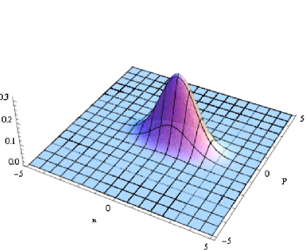
Figure 2:

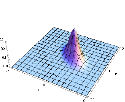
Figure 3:

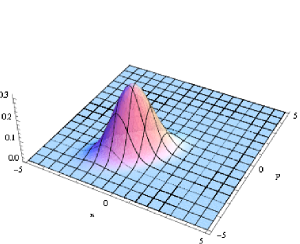
Figure 4: