Dispersion Management of Ultraslow Light in a Bose-Einstein Condensate via Trap Curvature

Abstract

One dimensional propagation of ultraslow optical pulses in an atomic Bose-Einstein condensate taking into account the dispersion and the spatial inhomogeneity is investigated. Analytical and semi-analytical solutions of the dispersive inhomogeneous wave equation modeling the ultraslow pulse propagation are developed and compared against the standard wave equation solvers based upon Cranck-Nicholson and pseudo-spectral methods. The role of curvature of the trapping potential of the condensate on the amount of dispersion of the ultraslow pulse is pointed out.

I Introduction

Possibility of dramatic reduction of speed of light, as demonstrated in an atomic Bose-Einstein condensate (BEC) slowlight-exp1 using electromagnetically induced transparency (EIT) eit1 , opens the way towards practical realization of quantum optical information storage qmemory1 ; qmemory2 ; qmemory3 ; qmemory4 ; liu . In BECs, ultraslow group velocities allow for storage times of coherent optical information of the order of few microseconds. To enhance the storage capacity and duration it is necessary to inject multiple pulses to be simultaneously present in the condensate. Major limiting factor against this goal is the narrow EIT window and group velocity dispersion of the slow pulses.

Propagation of the ultraslow wave packet in one dimensional inhomogeneous dispersive atomic condensate can be described in terms of the slowly varying pulse envelope tarhan1 ; tarhan2

$$\frac{\partial E}{\partial z}+\alpha(z)E+\frac{1}{v_{g}(z)}\frac{\partial E}{\partial t}+i\,b_{2}(z)\frac{\partial^{2}E}{\partial t^{2}}=0,$$ (1)

where $\alpha(z)$ is the pulse attenuation factor; $v_{g}(z)$ is the group velocity, and $b_{2}(z)$ is the group velocity dispersion. The third order dispersion is found to be much smaller and neglected tarhan2 . Previous studies are based upon either analytical solutions obtained for an effective homogeneous region at the center of the condensate where the dispersion is highest or numerical propagation of the pulse with the standard methods such as Cranck-Nicolson or pseudo-spectral schemes tarhan2 .

Present work aims to solve Eq. (1) analytically so that optimum experimental conditions can be efficiently determined to reduce the dispersive effects to enhance coherent information storage capacity of the condensate. In addition to exact analytical expressions of the pulse envelopes, an approximate method of determination of the pulse envelope by polynomial or Gaussian function fitting to condensate density profile is introduced. The density profile only contributes as an integrand to the optical parameters so that the fitting can be done with very high accuracy for a simple and fast evaluation of the required integrals. Besides, the spatial dependence of the coefficients in the wave function is due to the inhomogeneous condensate profile for which non-condensate, thermal component makes a small contribution at low temperatures. The practical semi-analytical approach outlined as above is tested against Cranck-Nicolson and pseudo-spectral wave equation solvers and shown to be highly efficient. The approach is employed to investigate the effect of the curvature of the trapping potential of the condensate, translated to the curvature of the dielectric function of the condensate, on the amount of the dispersion of the optical pulse.

The paper is organized as follows: In Sec. II, optical properties of an atomic BEC system under EIT conditions is briefly reviewed. In Sec. III, analytical and semi-analytical solutions are developed for the wave equation. Numerical schemes used against the semi-analytical solution are described in Sec. IV. Results are discussed in Sec.V. Finally, we conclude in Section VI.

II Optical properties of an atomic BEC under EIT conditions

Atomic condensates can be considered as two component objects, composed of a condensate cloud in a thermal background so that one can write its density being

$$\rho(\vec{r})=\rho_{c}(\vec{r})+\rho_{T}(\vec{r}),$$ (2)

where naraschewski

$$\rho_{c}(\vec{r}) = \frac{\mu-V(r)}{U_{0}}\Theta(\mu-V(r))\Theta(T_{c}-T),$$ (3)

$$\rho_{T}(\vec{r}) = \frac{g_{3/2}(ze^{-\beta V})}{\lambda_{T}^{3}}.$$ (4)

Here $U_{0}=4\pi\hbar^{2}a_{s}/m$, $m$ is atomic mass, and $a_{s}$ is the atomic s-wave scattering length. $\Theta(.)$ is the Heaviside step function, $g_{n}(x)=\Sigma_{j}x^{j}/j^{n}$, $\lambda_{T}$ is the thermal de Bröglie wavelength, $\beta=1/k_{B}T$, and $T_{C}$ is the critical temperature. We assume an external trapping potential in the form $V(\vec{r})=(1/2)m(\omega_{r}^{2}r^{2}+\omega_{z}^{2}z^{2})$ with $\omega_{r}$ the radial trap frequency and $\omega_{z}$ the axial trap frequency in the z direction. $\mu$ is the chemical potential. At temperatures below $T_{c}$, the chemical potential $\mu$ is determined by $\mu(T)=\mu_{TF}(N_{0}/N)^{2/5}$, where $\mu_{TF}$ is the chemical potential evaluated under Thomas-Fermi approximation. The condensate fraction is evaluated by naraschewski $N_{0}/N=1-x^{3}-s\zeta(2)/\zeta(3)x^{2}(1-x^{3})^{2/5}$, with $x=T/T_{c}$, and $\zeta$ is the Riemann-Zeta function. The scaling parameter $s$ is given by $s=\mu_{TF}/k_{B}T_{C}$.

EIT susceptibility eit2 for an atomic BEC of atomic density $\rho$ can be expressed as $\chi(\vec{r},\omega)=\rho(\vec{r})\chi_{1}(\omega)$ with

$$\chi_{1}(\omega)=\frac{|\gamma|^{2}}{\epsilon_{0}\hbar}\frac{{\rm i}(\Gamma_{2}/2-{\rm i}\Delta)}{[(\Gamma_{2}/2-{\rm i}\Delta)(\Gamma_{3}/2-{\rm i}\Delta)+\Omega_{c}^{2}/4]},$$ (5)

where $\Delta=\omega-\omega_{0}$ is the detuning of the probe field frequency $\omega$ from the atomic resonance $\omega_{0}$. $\Omega_{c}$ is the Rabi frequency of the control field; $\gamma$ is the dipole matrix element for the probe transition. $\Gamma_{2}$ and $\Gamma_{3}$ denote the dephasing rates of the atomic coherence.

Through the atomic density, the optical response of the atomic condensate becomes spatially inhomogeneous, so does the parameters in the wave equation (1). They are determined by harris

$$\alpha(\vec{r}) = -\frac{i\pi}{\lambda}\rho(\vec{r})\chi_{1}(\omega_{0}),$$

$$\frac{1}{v_{g}(\vec{r})} = \frac{1}{c}-\frac{\pi}{\lambda}\rho(\vec{r})\left.\frac{\mathrm{d}\chi_{1}}{\mathrm{d}\omega}\right|_{\omega_{0}},$$ (6)

$$b_{2}(\vec{r}) = \frac{\pi}{2\lambda}\rho(\vec{r})\left[\left.\frac{\mathrm{d}^{2}\chi_{1}}{\mathrm{d}\omega^{2}}\right|_{\omega_{0}}\right].$$

Thus the spatial dependence of all the optical parameters comes solely from the axial density profile of the condensate. In the following section we shall exploit the fact that it is only the density profile that determines the local optical properties of the condensate to develop an exact analytical solution of the wave Eq.(1).

III Analytical and Semi-Analytical Methods for ultraslow pulse propagation

For a uniform density medium the Eq.1 can be solved analytically bahaa . The complex envelope of the incident wave is Gaussian pulse $E(0,t)=e^{-t^{2}/\tau_{0}^{2}}$. The initial pulse, after propagating in the medium of length $L$, is then found to be delayed with respect to a reference pulse propagating in vacuum by $t_{d}=L/v_{g}$. The final width of the pulse is $\tau(L)=\tau_{0}\sqrt{1+(L/z_{0})^{2}}$ with $\tau_{0}$ is the initial temporal width of the pulse, and $z_{0}=-\pi\tau_{0}^{2}/b_{2}$. For $L\gg z_{0}$ we get $\tau(L)=|b_{2}|L/\pi\tau_{0}$. Experimentally measured group velocity is defined by $v_{g}=L/t_{d}$, where the effective axial length of the medium is evaluated by $L=\left[(4\pi/N)\int_{0}^{\infty}\,r\mathrm{d}r\int_{0}^{\infty}\,\mathrm{d}zz^{2}\rho(r,z)\right]^{1/2}$.

For a non-uniform medium, the wave equation (1) with spatial dependent coefficients can be solved by using some basic differential equation solving methods. In the typical slow light experiments a small pin hole is introduced to couple incoming light with the condensate guide and axial propagation is enforced. In the subsequent discussions paraxial effects shall be ignored and strictly one dimensional propagation will be considered by taking $\vec{r}=(x,y,z)=(0,0,z)$. Fourier transforming Eq. (1) from $t$ space to $w$ space gives

$$\frac{\mathrm{d}{\cal E}}{\mathrm{d}z}+\alpha(z){\cal E}-\frac{{\rm i}w}{v_{g}(z)}{\cal E}-w^{2}{\rm i}b_{2}(z){\cal E}=0$$ (7)

where ${\cal E}={\cal E}(z,w)\equiv(1/\sqrt{2\pi})\int_{-\infty}^{\infty}E(z,t)\exp{({\rm i}wt)}\mathrm{d}\,t$. Solution for the equation in $w$ space becomes

$${\cal E}(z,w)={\cal E}_{0}\;\exp{\left[\int^{z}\left({\rm i}w^{2}b_{2}(z^{\prime})+{\rm i}w/v_{g}(z^{\prime})-\alpha(z^{\prime})\right)\mathrm{d}\,z^{\prime}\right]},$$ (8)

where ${\cal E}_{0}=(1/\sqrt{2\pi})\int_{-\infty}^{\infty}\exp{(-(t-t_{0})^{2}/2\tau_{0}^{2})}\exp{({\rm i}wt)}\mathrm{d}t=\tau_{0}\exp{(-w^{2}\tau_{0}^{2}/2)}$. Transforming back to $t$ space we find

$$E(z,t)=\frac{\tau_{0}}{\sqrt{2f_{1}(z)}}\exp{\left[-\int^{z}\alpha(z^{\prime})\mathrm{d}z^{\prime}-\frac{f_{2}^{2}(z)}{4f_{1}(z)}\right]},$$ (9)

where

$$f_{1}(z) = \left(\frac{\tau_{0}^{2}}{2}-\int^{z}b_{2}(z^{\prime})\mathrm{d}z^{\prime}\right),$$ (10)

$$f_{2}(z) = \left(t-t_{0}-\int^{z}\frac{1}{v_{g}(z^{\prime})}\mathrm{d}z^{\prime}\right).$$ (11)

Writing the trap potential with a variable curvature parameter $\kappa$ such that $V=\kappa z^{2}$, density profile of 1D Bose-Einstein condensate becomes $\rho(z)=[(\mu-V(z))/U_{0}]\Theta(\mu-\kappa z^{2})+g_{3/2}(\exp{(-\beta(\kappa z^{2}-\mu))})/\lambda_{T}^{3}.$ To calculate the pulse envelope analytically, it is necessary to be able to evaluate the single integral

$$N(z)=\int_{-\infty}^{z}\rho(z^{{}^{\prime}})\mathrm{d}z^{{}^{\prime}}=N_{0}(z)+N_{T}(z),$$ (12)

with $N_{0}(z)=\int_{-\sqrt{\mu/\kappa}}^{z}\rho_{0}(z^{{}^{\prime}})\mathrm{d}z^{{}^{\prime}}$ and $N_{T}(z)=\int_{-\infty}^{z}\rho_{T}(z^{{}^{\prime}})\mathrm{d}z^{{}^{\prime}}$. $N_{0}$ makes the dominant contribution in the condensate region. Let us define an auxiliary function for notational simplicity such that

$$F(z)=\frac{1}{\lambda_{T}^{3}}\sum_{j=1}^{\infty}\sqrt{\frac{\pi}{\beta\kappa}}\frac{e^{\beta\mu j}}{j^{2}}\phi(\sqrt{2\beta\kappa j}z),$$ (13)

where $\phi(x)=1/(\sqrt{\pi})\int_{-\infty}^{x}e^{-u^{2}/2}\mathrm{d}u$ is the normal cumulative distribution function which can be expressed in terms a tabulated special function, error function as $\phi(x)=1/2(1+\mathrm{erf}(x/\sqrt{2}))$. It is now possible to express the results of the integral as follows

$$N(z)=\cases{F(z)&$z<-|z_{0}|$\cr\frac{2}{3U_{0}}\sqrt{\frac{\mu^{3}}{\kappa}}+\frac{\mu z-\kappa z^{3}/3}{U_{0}}+F(-|z_{0}|)&$z\in(-|z_{0}|,|z_{0}|)$\cr\frac{4}{3U_{0}}\sqrt{\frac{\mu^{3}}{\kappa}}+F(z)&$z>|z_{0}|$}.$$ (14)

Here $|z_{0}|=\sqrt{\mu/\kappa}$. Finally we can rewrite optical pulse parameters in terms of $N(z)$ so that

$$f_{1}(z) = \left(\frac{\tau_{0}^{2}}{2}-\frac{\pi}{2\lambda}\left.\frac{\mathrm{d}^{2}\chi_{1}}{\mathrm{d}\omega^{2}}\right|_{\omega_{0}}N(z)\right)$$ (15)

$$f_{2}(z) = \left(t-t_{0}-\frac{z}{c}+\frac{\pi}{\lambda}\left.\frac{\mathrm{d}\chi_{1}}{\mathrm{d}\omega}\right|_{\omega_{0}}N(z)\right)$$ (16)

$$\bar{\alpha}(z) = \left(-\frac{i\pi}{\lambda}\chi_{1}(\omega_{0})N(z)\right).$$ (17)

This completes our analytic exact solution. Though it contains an infinite series, not all terms would be of significance at condensate temperatures of interest. Furthermore one can still make the result of more practical value by noting that it contains a special function. In addition to its series and asymptotic expansions, there are elementary, Gaussian-like functions that can be fit to the error function. Thus these facts encourage us to look for a semi-analytical method in which we fit polynomials or Gaussian to the $N(z)$. Equivalently and more simply then one can make such fits to the density profile of the condensate. Its exact form is not essential as it only appears as an integrand. Due to the approximate fitting involved, this method would be a semi-analytical method to determine the pulse envelope. After quickly reviewing standard numerical solvers of wave equation such as Cranck-Nicolson and spectral methods, we shall test the semi-analytical method against them.

IV Typical Numerical methods for pulse propagation

IV.1 Crank-Nicolson Method

A dimensionless form of Eq. (1) can be solved via finite difference Crank-Nicolson space marching scheme. The Crank-Nicolson scheme is less stable but more accurate than the fully implicit method; it takes the average between the implicit and the explicit schemes Garcia . Discritization is performed as follows, with $i,j$ being the space and time grid variables $(i,j=0,1,...,N)$ and $E(z,t)\equiv E_{j}^{i}$,

$$\frac{\partial E}{\partial z} = \frac{E_{j}^{i+1}-E_{j}^{i}}{\Delta z};\quad\quad\frac{\partial E}{\partial t}=\frac{E_{j+1}^{i}-E_{j-1}^{i}}{2\Delta t};$$

$$\frac{\partial^{2}E}{\partial t^{2}} = \frac{1}{2(\Delta t)^{2}}([E_{j+1}^{i}+E_{j-1}^{i}-2E_{j}^{i}]$$ (18)

$$+ [E_{j+1}^{i+1}+E_{j-1}^{i+1}-2E_{j}^{i+1}]).$$

If we plug them into the wave equation (1), we get

$$\frac{ib_{2}}{2(\Delta t)^{2}}E_{j-1}^{i+1}+\left(\frac{1}{\Delta z}-\frac{ib_{2}}{(\Delta t)^{2}}\right)E_{j}^{i+1}+\frac{ib_{2}}{2(\Delta t)^{2}}E_{j+1}^{i+1}$$

$$=\left(-\frac{1}{2v_{g}\Delta t}-\frac{ib_{2}}{2(\Delta t)^{2}}\right)E_{j-1}^{i}+$$

$$\left(\alpha-\frac{1}{\Delta z}-\frac{ib_{2}}{(\Delta t)^{2}z}\right)E_{j}^{i}+\left(\frac{ib_{2}}{2(\Delta t)^{2}}+\frac{1}{2v_{g}\Delta t}\right)E_{j+1}^{i}$$ (19)

By adding the boundary conditions (in our work set as zero: $E_{0}^{i}=E_{N-1}^{i}=0$ for all $"i"$) we obtain set of $N$ linear equations with $N$ unknowns, which have to be solved simultaneously for every space step $i$ where the vector $\{E_{0}\}$ is defined by initial conditions. Discrete equations in matrix form are solved using Thomas algorithm Garcia which is a fast Gaussian elimination method for tridiagonal matrices.

IV.2 Pseudo-spectral Method

Instead of doing a finite difference approximation in time, we can expand the function $E(z,t)$ in spectral series at a given position for all time values for better approximation of the time derivative. The initial value can be used to determine the coefficients of spectral series Boyd ; Tref . An appropriate spectral series can be Fourier series. The reason we choose Fourier series instead of polynomials or any other series that the derivative of the Fourier series is just multiplication of Fourier series with a pre-defined vector and also fast Fourier algorithm makes it faster to compute the Fourier coefficients.

The initial function is divided into N points ($E_{j}$) and discrete Fourier transform is applied in the interval $-N/2\leq k\leq N/2-1$.

$$E_{k}=\mathcal{F}\{E_{j}\}=\frac{1}{N}\sum_{j=0}^{N-1}E_{j}e^{-i2\pi kj/N}\quad$$ (20)

for all k. We get the following ordinary differential equation;

$$\frac{\partial E(z,k)}{\partial z}=-\left(\alpha+\frac{ik}{v_{g}}-ib_{2}k^{2}\right)E(z,k)$$ (21)

We solve this ordinary differential equation for discrete space intervals assuming that for each interval coefficients are constants;

$$E(z_{0}+\Delta z,k)=E(z=z_{0},k)\cdot e^{\Delta z(-\alpha-\frac{ik}{v_{g}}+ib_{2}k^{2})}$$ (22)

V Results and discussion

In our numerical calculations, we specifically consider a gas of $N=8.3\times 10^{6}$ ²³Na atoms for which $M=23$ amu, $\lambda_{0}=589$ nm, $\gamma=2\pi\times 10.01$ MHz, $\Gamma_{3}=0.5\gamma$, $\Gamma_{2}=2\pi\times 10^{3}$ Hz, and $a_{s}=2.75$ nm. For the parameters of the trapping potential, we take $\omega_{r}=2\pi\times 69$ Hz and $\omega_{z}=2\pi\times 21$ Hz as in Ref. slowlight-exp1 . The coupling field Rabi frequency is taken to be $\Omega_{c}=0.56\gamma$ slowlight-exp1 . Critical temperature for Bose-Einstein condensation of such a gas is found to be $T_{C}=424$ nK.

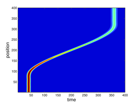
Figure 2: Contour graph of the propagation of a microsecond pulse through the interacting BEC by semi-analytical method. Time ($t$) is scaled by $0.22\,\mu$s. and position ($z$) is scaled by $1\,\mu$m. The parameters are the same with those of Fig.1.

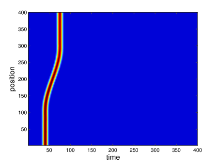
Figure 3: Contour graph of the propagation of a microsecond pulse through the interacting BEC by semi-analytical method. Time ($t$) is scaled by $0.22\,\mu$sec. and position ($z$) is by $1\,\mu$m. The parameters are the same with those of Fig.1 except for $\Omega_{c}=1.5\gamma$.

Fitting a polynomial of degree $22$, pulse envelope is calculated using the analytical formulae. To illustrate the success of the fit we present the absorption coefficient in Fig.(1) at temperature $T=42$ nK. Solid line is the exact analytical absorption coefficient while the dot line is the semi-analytical result obtained after the polynomial fit. Similar behavior occurs for $b_{2}$ and $1/v_{g}$. With the polynomial expressions of the optical parameters, the integrals required for pulse envelope functions such as $f_{1,2}$, or $N(z)$, are evaluated quickly and simply. Contour plots of the propagating pulse are shown in Figs. 2-3. We assume a Gaussian pulse with unit amplitude of the form $\exp{(-(t-t_{0})^{2}/2\tau_{0}^{2})}$ at initial time $t_{0}$, , where $\tau_{0}$ is the pulse width. When the optical pulse enters the condensate region, its group speed dramatically reduces under EIT conditions, as shown in Fig. 2. The optical pulse rapidly assumes its high speeds again following the passage to the thermal background cloud. We assumed the optical pulse is propagating in vacuum before and after the thermal component of the ultracold atomic system. In experiment, group velocity is measured in terms of time delay of the pulse with respect to a reference pulse which propagates in vacuum over the same distance with the atomic medium. Broadening of the pulse after leaving the condensate is visibly seen in the figure as it gets about almost two times broader.

Similar behavior of the pulse but with a significant difference regarding the pulse width can be seen in the Fig. 3. The only change in the parameters used in Fig. 2 is that now $\Omega_{c}=1.5\gamma$. In that case the broadening and absorption becomes negligible while the pulse gets faster. These results, in particular the role of the intensity of the control field on the dispersion and loss management have already been discussed before in Ref. tarhan2 . Here, the semi-analytical method is shown to reproduce them efficiently.

To test the semi-analytical method with polynomial fitting against standard numerical solvers of the wave equation, a dimensionless form of Eq. (1) is also solved via finite difference Crank-Nicolson (C-N) space marching scheme and pseudo-spectral method (P-S). Final pulse width and final amplitude determined by these methods are listed in Tab.(1). A microsecond pulse broadens by a factor of approximately $\sim 1.7$ according both numerical and semi-analytical methods as seen in Tab.(1). Similar agreement of the semi-analytical method with the numerical results are found for the absorption loss.

As a further test on our numerical methods as well, we have compared the results of the Crank-Nicolson and pseudo-spectral codes against the exact analytical solution for a uniform density condensate cloud of $\rho=1.56\times 10^{20}$ 1/m³. The coefficients in the Eq. (1) in that case are found to be $v_{g}=1.5$ m/s, $\alpha=2.1\times 10^{3}$ 1/m, and $b_{2}=3.39\times 10^{-8}$ s²/m. Initial value for pulse width is $1\,\mu$sec. The final pulse width determined according to the Crank-Nicolson, pseudo-spectral, and completely analytic methods are $3.3863\,\mu$sec, $3.3861\,\mu$sec, and $3.3869\,\mu$sec respectively.

We can also use Gaussian fitting functions instead of polynomials in order to get more explicit and compact expressions. Fitting a Gaussian to the density for the same experimental parameters, we have found the optical parameters become

$$\alpha(z)=2.25\times 10^{-3}\exp{\left[{-\frac{(z-1.5\times 10^{-4})^{2}}{0.25\times 10^{-8}}}\right]},$$

$$b_{2}(z)=-1.15\times 10^{-8}\exp{\left[{-\frac{(z-1.5\times 10^{-4})^{2}}{0.25\times 10^{-8}}}\right]},$$ (23)

$$1/v_{g}(z)=0.71\times\exp{\left[{-\frac{(z-1.5\times 10^{-4})^{2}}{0.25\times 10^{-8}}}\right]}.$$

Reliability of the Gaussian fitting in the semi-analytical method is tested against spectral method and Crank-Nicolson method as summarized in Tab.(2) and Tab.(3). Results obtained with numerical or semi-analytical Gaussian fit methods are found to be in good agreement among themselves. Furthermore, Gaussian fit method gives the similar results obtained with the polynomial fit. This should be the case as the density only enters as an integrand and the exact shape of the density should not be essential to determine the optical pulse properties. Gaussian fit method gives the final amplitude and width to be $0.475$ and $1.7524\,\mu$sec, respectively. In these tables we have seen that the agreement between the semi-analytical method and the numerical methods seems to improve as the grid made finer and finer. This may suggest that the semi-analytical method is more accurate than the standard numerical solvers. However we are unable to give more rigorous proof for that statement than these numerical tests.

Having analytical pulse envelope expressions or its reliable and compact semi-analytical form allows us to vary controllable experimental parameters easily to optimize pulse width, group velocity and absorption loss of the pulse. To illustrate such optimum dispersion management, we choose to examine the effect of the trap curvature to illustrate. Effect of the control field intensity has been numerically investigated earlier tarhan2 . Considering a quadratic trap as $V=\kappa z^{2}$, trap curvature is translated to the curvature of the dielectric function through the density dependent EIT susceptibility. Typical results obtained by the Gaussian fitting semi-analytical method are listed in listed in Tab.(4). The parameters are the same with those of Fig.1 and $\kappa$ is in units of kg/sec². It is seen that pulse shape is better preserved at larger $\kappa$.

VI Conclusion

We have discussed analytical and semi-analytical solution of the one -dimensional wave equation which governs the propagation of an ultraslow optical pulse in a dispersive inhomogeneous atomic condensate. Ignoring paraxial effects, slowly varying pulse envelope wave equation is solved by using Fourier transformation technique and by using special functions, in particular, normal cumulative distribution function which is related to the error function. It has been argued that, as the exact density profile only enters as an integrand to the expressions, simpler polynomial and Gaussian fits can be made for more compact and simpler expressions. Such a semi-analytical method is heavily tested against standard numerical solvers of the wave equation, namely, Cranck-Nicolson and pseudo-spectral methods. The results confirm the reliability of the compact expressions obtained under semi-analytical method. As an illustration of the efficiency of analytical expressions, the role of trap curvature on the dispersion management has been investigated. A quick calculation shows that pulse shape is more preserved in traps with higher curvatures. Other experimentally controllable parameters can be similarly studied for optimized design of optical traps and EIT conditions to efficient storage of coherent optical information or to engineer ultraslow pulse shapes.

List of Figure Captions

Fig. 1. Solid line shows the position dependence of the absorption coefficient $\alpha$ along the $z$-axis. The dot line is polynomial fitting for the absorption coefficient and the degree of the polynomial is 22. The ultracold atomic system of ²³Na $N=8.3\times 10^{6}$ atoms at $T=42$ nK under EIT scheme. The parameters used are $M=23$ amu, $a_{s}=2.75$ nm, $\lambda_{0}=589$ nm, $\gamma=2\pi\times 10.01$ MHz, $\Gamma_{3}=0.5\gamma$, $\Omega_{c}=0.56\gamma$, $\Gamma_{2}=2\pi\times 10^{3}$ Hz.

Fig. 2. Contour graph of the propagation of a microsecond pulse through the interacting BEC by semi-analytical method. Time ($t$) is scaled by $0.22\,\mu$s. and position ($z$) is scaled by $1\,\mu$m. The parameters are the same with those of Fig.1

Fig. 3. Contour graph of the propagation of a microsecond pulse through the interacting BEC by semi-analytical method. Time ($t$) is scaled by $0.22\,\mu$sec. and position ($z$) is by $1\,\mu$m. The parameters are the same with those of Fig.1 except for $\Omega_{c}=1.5\gamma$.

List of Table

Table 1: Comparison of Crank-Nicolson (C-N), pseudo-spectral (P-S), and semi-analytical (S-A) method. Propagation of optical pulse with initial pulse width $1\,\mu$sec and initial amplitude $1$.

	C-N	P-S	S-A
final pulse width	$1.7311\,\mu$sec0	$1.7305\,\mu$sec0	$1.7309\,\mu$sec0
final amplitude	0.47550	0.47540	0.47580

Table 2: Ratio of the results for pseudo-spectral method to the semi-analytical values for the given position$\times$time grid dimensions.

grid dimensions	final amplitude	final width
$2^{9}\times 2^{9}$	0.998	0.9993
$2^{10}\times 2^{10}$	0.9993	0.9997
$2^{12}\times 2^{10}$	0.9995	0.9998
$2^{12}\times 2^{12}$	0.9998	0.99991

Table 3: Ratio of the results for Crank-Nicolson method to the semi-analytical values for the given position$\times$time grid dimensions.

grid dimensions	final amplitude	final width
$2^{9}\times 2^{9}$	0.9998	0.9994
$2^{12}\times 2^{10}$	0.99988	0.99991
$2^{12}\times 2^{12}$	0.99998	0.99994

Table 4: Dispersive propagation of optical pulse as a function of $\kappa$.

$\kappa$	final amplitude	final width ($\mu$sec)
$2\times 10^{-22}$	0.4113	1.8916
$0.5\times 10^{-21}$	0.5250	1.6247
$1\times 10^{-21}$	0.6121	1.4612
$0.5\times 10^{-20}$	0.7629	1.2422
$1\times 10^{-20}$	0.8212	1.1741

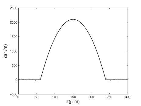
Figure 1: Solid line shows the position dependence of the absorption coefficient $\alpha$ along the $z$-axis. The dot line is polynomial fitting for the absorption coefficient and the degree of the polynomial is 22. The ultracold atomic system of ²³Na $N=8.3\times 10^{6}$ atoms at $T=42$ nK under EIT scheme. The parameters used are $M=23$ amu, $a_{s}=2.75$ nm, $\lambda_{0}=589$ nm, $\gamma=2\pi\times 10.01$ MHz, $\Gamma_{3}=0.5\gamma$, $\Omega_{c}=0.56\gamma$, $\Gamma_{2}=2\pi\times 10^{3}$ Hz.

References

- (1) L.V. Hau, S.E. Harris, Z. Dutton, and C.H. Behroozi, Nature 397, 594(1999).
- (2) S. E. Harris, Physics Today 50, 36 (1997).
- (3) M. Fleischhauer and M. D. Lukin, Phys. Rev. Lett. 84, 5094 (2000).
- (4) M. D. Lukin, S. F. Yelin, and M. Fleischhauer, Phys. Rev. Lett. 84, 4232 (2000).
- (5) M. D. Lukin and A. Imamoglu, Nature 413, 273 (2001).
- (6) D. F. Phillips, A. Fleischhauer, A. Mair, R. L. Walsworth , and M. D. Lukin, Phys. Rev. Lett. 86, 783 (2001).
- (7) C. Liu, Z. Dutton, C. H. Behroozi, and L. V. Hau, Nature 409, 490 (2001).
- (8) D. Tarhan, S. Sefi, and Ö. Müstecaplıog̃lu, J. Phys. Conf. Ser. 36, 194 (2006).
- (9) D. Tarhan, A. Sennaroglu, and Ö. Müstecaplıog̃lu, J. Opt. Soc. Am. B 23, 1925 (2006).
- (10) M. Naraschewski, D. M. Stamper-Kurn, Phys. Rev. A 58, 2423 (1998).
- (11) M. O. Scully and M. S. Zubairy, Quantum Optics (Cambridge Univ. Press, Cambridge, 1997).
- (12) S. E. Harris, J. E. Field, and A. Kasapi, Phys. Rev. A 46, R29 (1992).
- (13) B. E. A. Saleh and M. C. Teich, Fundamentals of photonics, John Wiley and Sons, New York, 1991.
- (14) A. L. Garcia, Numerical methods for physics, Prentice Hall, Newyork, 2000.
- (15) J. P. Boyd, Chebyshev and Fourier Spectral Methods, (Dover Publications, New York, 2000).
- (16) L. N. Trefethen, Spectral Methods in Matlab, (SIAM, Philadelphia, 2000).