Two-component jet simulations

Abstract

Context. Theoretical arguments along with observational data of YSO jets suggest the presence of two steady components: a disk wind type outflow needed to explain the observed high mass loss rates and a stellar wind type outflow probably accounting for the observed stellar spin down. Each component’s contribution depends on the intrinsic physical properties of the YSO-disk system and its evolutionary stage.

Aims. The main goal of this paper is to understand some of the basic features of the evolution, interaction and co-existence of the two jet components over a parameter space and when time variability is enforced.

Methods. Having studied separately the numerical evolution of each type of the complementary disk and stellar analytical wind solutions in Paper I of this series, we proceed here to mix together the two models inside the computational box. The evolution in time is performed with the PLUTO code, investigating the dynamics of the two-component jets, the modifications each solution undergoes and the potential steady state reached.

Results. The co-evolution of the two components, indeed, results in final steady state configurations with the disk wind effectively collimating the inner stellar component. The final outcome stays close to the initial solutions, supporting the validity of the analytical studies. Moreover, a weak shock forms, disconnecting the launching region of both outflows with the propagation domain of the two-component jet. On the other hand, several cases are being investigated to identify the role of each two-component jet parameter. Time variability is not found to considerably affect the dynamics, thus making all the conclusions robust. However, the flow fluctuations generate shocks, whose large scale structures have a strong resemblance to observed YSO jet knots.

Conclusions. Analytical disk and stellar solutions, even sub modified fast ones, provide a solid foundation to construct two-component jet models. Tuning their physical properties along with the two-component jet parameters allows a broad class of realistic scenarios to be addressed. The applied flow variability provides very promising perspectives for the comparison of the models with observations.

1 Introduction

Jets are supersonic and highly collimated plasma outflows emanating from a plethora of astrophysical objects. In particular, those associated with Young Stellar Objects (YSO) have been found to be accretion powered (Cabrit et al.Cab90 (1990); Hartigan et al. Har95 (1995)), to have narrow opening angles and to propagate for several hundreds of AU (Dougados et al. Dou00 (2000); Hartigan et al. Har04 (2004)). Although their large scale properties are rather well known, the conditions at the launch regions are still unclear. The new generation of high angular resolution instrumentation is expected to adequately resolve the central regions of YSOs and hence constrain the various theoretical models that currently exist.

A promising scenario supported by both observational data and theoretical arguments is that of a two-component jet, wherein a pressure driven stellar outflow is surrounded by a disk wind. In particular, He i $\lambda 10830$ profiles of classical T Tauri stars (CTTS) indicate the presence of two genres of wind (Edwards et al. Edw06 (2006); Kwan et al. Kwa07 (2007)). One is ejected radially with respect to the central object and the other is launched at a constant angle with respect to the equatorial plane. As a result, CTTS may be classified according to their outflow properties. Some of them seem to be associated with a stellar origin, others with a disk origin and the rest with both components having roughly equivalent contributions. Therefore, it is suggested that both types of winds participate, with the dominance being dictated by the intrinsic physical factors of the specific YSO.

Such a scenario (e.g. Sauty & Tsinganos Sau94 (1994); Shu et al. Shu94 (1994)) is supported by theoretical arguments as well. Ferreira et al. (Fer06 (2006)) conclude that YSO jets consist of two types of steady winds plus a sporadic outflow. An extended disk wind, which is required for the explanation of the high mass fluxes observed in optical jets and an inner pressure driven outflow of stellar origin (Bogovalov & Tsinganos Bog01 (2001)) collimated by the disk wind. A third component is expected to be launched due to the variable conditions of the thin layer between the protostellar magnetosphere and the disk’s magnetic field. Their interaction may drive weak sporadic mass ejections probably associated with jet variability.

In favor of the two-component jet scenario, there is also the yet unresolved question of the protostellar spin down. Matt & Pudritz (Mat05 (2005); 2008a ; 2008b ) have shown that the disk-locking mechanism, which was believed to slow down the rotation of the central object, is not in good agreement with observations. On the contrary, they propose that the stellar wind is capable of and most likely responsible for the spin down of the protostar. A wide parameter space has been investigated to support such a conclusion, whereas it is argued that the physical mechanisms which drive the actual launching are less important, hence allowing all sorts of stellar wind models.

A plethora of studies exists in the literature concerning numerical simulations performed to investigate the launching and propagation of jets. Two approaches are adopted: in the one, the disk is treated as a boundary (e.g. Pudritz et al. Pud06 (2006); Fendt Fen06 (2006); and references therein), while in the other the disk is included in the computational box, hence studying its dynamics simultaneously and self consistently with those of the jet (first studied in Casse & Keppens Cas02 (2002), Cas04 (2004)). More recently, Meliani et al. (Mel06 (2006)) effectively incorporated a stellar type outflow accelerated by turbulent heating and in Meliani & Keppens (Mel07 (2007)), the transverse stability of relativistic two-component jets was examined. Furthermore, adopting a different initial setup, Zanni et al. (Zan07 (2007)) studied the effects of resistivity on the dynamics of the disk-jet system and Tzeferacos et al. (submitted ) performed an interesting parameter study on disk magnetization.

Despite the complexity of the non-linear MHD equations, the derivation of analytical steady state outflow solutions has proved successful in the context of self-similarity (Vlahakis & Tsinganos Vla98 (1998)). Each family of these solutions (radially or meridionally self-similar) manages to capture the physical mechanisms involved in either disk winds (Blandford & Payne Bla82 (1982); Ferreira Fer97 (1997); Vlahakis et al. Vla00 (2000), hereafter VTST00), or stellar outflows (Sauty & Tsinganos Sau94 (1994); Trussoni et al. Tru97 (1997); Sauty et al. Sau02 (2002), hereafter STT02). The geometrical properties of these two classes of solutions are complementary. Although radially self-similar models become singular at small polar angles, the meridionally self-similar ones are by definition appropriate for modeling of the outflow at the axis.

In the first paper of this series (Matsakos et al. Mat08 (2008), Paper I), we addressed the topological stability, as well as several physical and numerical properties, separately for typical radially and meridionally self-similar solutions. Such analytically derived wind models were defined as ADO (Analytical Disk Outflow) and ASO (Analytical Stellar Outflow), respectively.

Concerning the ADO model, its main feature is the formation of a shock in the super fast magnetosonic region. Upstream of this shock, the analytical and the asymptotic numerical solutions are basically coincident, while the downstream flow converges to a consistent physical solution, overcoming the singularity of the analytical model at the symmetry axis (first achieved in Gracia et al. Gra06 (2006)). This shock corresponds to the numerically modified fast magnetosonic separatrix surface (FMSS, Tsinganos et al. Tsi96 (1996)) that causally disconnects the downstream flow from its launching region. This property is quite robust to variation of the physical parameters, and has been recently confirmed also in Stute et al. (Stu08 (2008)), where an outer radial truncation of the disk wind was imposed in the simulations. Moreover, a particular model was initialized by specifying a sub modified fast solution both at the initial conditions and at the boundaries (i.e. a flow causally connected throughout the whole computational domain). Over time, the shock was still found, with its position marking the FMSS that causally separates the upstream and downstream regions.

On the contrary, the ASO model does not show singularities at its boundaries and therefore, the evolution of its super Alfvénic region does not show any readjustments. However, since energy input is a vital constituent of the model’s acceleration, the modifications of the energy source terms in the sub Alfvénic domain were demonstrated to strongly affect the outcome of the flow. In particular, we verified that an adiabatic evolution resulted in a collapse of the jet to an almost static atmosphere, whereas specifying a polytropic index to mimic almost isothermal conditions produces a weak collimated turbulent wind.

The goal of the present work is to study the two-component jet scenario, taking advantage of both analytical and numerical approaches. Specifically, we construct models by properly defining the initial conditions with a mixture of two analytical (ADO & ASO) solutions connected through a transition region. The introduction of a few normalization and mixing parameters, along with enforced time variability applied to the stellar component or at the matching surface, allows the examination of several interesting cases.

The paper is structured as follows. Section §2 revises a few basic properties of the analytical solutions, section §3 describes the mixing procedure followed to set the initial conditions. In the same section, the different cases investigated are presented along with the numerical setup. In section §4 we discuss the results of the simulations performed. Section §5 summarizes and reports the conclusions of this work.

2 MHD equations and the analytical solutions

Our starting point is the ideal MHD equations for the conservation of mass, momentum, energy and magnetic flux together with the flux-freezing condition:

$$\frac{\partial\rho}{\partial t}+\nabla\cdot(\rho\@vec{V})=0\,,$$ (1)

$$\frac{\partial\@vec{V}}{\partial t}+(\@vec{V}\cdot\nabla)\@vec{V}+\frac{1}{\rho}\@vec{B}\times(\nabla\times\@vec{B})+\frac{1}{\rho}\nabla P=-\nabla\Phi\,,$$ (2)

$$\frac{\partial P}{\partial t}+\@vec{V}\cdot\nabla P+\Gamma P\nabla\cdot\@vec{V}=\Lambda\,,$$ (3)

$$\frac{\partial\@vec{B}}{\partial t}-\nabla\times(\@vec{V}\times\@vec{B})=0\quad\mathrm{and}\quad\nabla\cdot\@vec{B}=0\,,$$ (4)

where $\rho$, $P$, $\@vec{V}$, $\@vec{B}$ are the density, pressure, velocity and magnetic field (over $\sqrt{4\pi}$), respectively. The gravitational potential, $\Phi,$ is equal to $-\mathcal{GM}/R$ with $\mathcal{G}$, $\mathcal{M}$ and $R$ denoting the gravitational constant, the mass of the central object and the spherical radius, respectively. $\Lambda$ represents the volumetric energy gain/loss terms ($\Lambda=[\Gamma-1]\rho\mathcal{Q}$, with $\mathcal{Q}$ the energy source terms per unit mass), and $\Gamma$ is the ratio of the specific heats.

Assuming steady state conditions and axisymmetry, several conserved quantities exist along the fieldlines (e.g. Tsinganos Tsi82 (1982)). These are the mass to magnetic flux ratio $\Psi_{A}$, the angular velocity of the footpoints of the fieldlines $\Omega$ and the total angular momentum flux to mass flux ratio $L$. If $\Lambda=(\Gamma-\gamma)P\nabla\cdot\@vec{V}$, where $\gamma$ is the polytropic index (see §3.4), also the total energy flux to mass flux $E$ and the specific entropy $Q$ are conserved along the streamlines.

In the paper we adopt the following notation: subscripts $D$ and $S$ are used to refer to the ADO and ASO solutions, respectively, while $(r,\phi,z)$ and $(R,\theta,\phi)$ are the cylindrical and spherical coordinates. Note that in Paper I the subscript $r$ was used for the ADO model and $\theta$ for the ASO solution. The subscript $*$ denotes a constant of the order of unity which is used for the relative normalization of the two solutions in order to correspond, for instance, to a solution of the same protostellar mass, as will be explained in §3. The values of the starred quantities correspond to the non-dimensional physical variables at the Alfvénic surfaces of each model at the reference fieldline $\alpha=1$ (see below). Finally, subscript zero in a quantity $U_{0}$ is used to introduce dimensions in the code units $U$, i.e. $U^{\prime}=U_{0}U$, where $U^{\prime}$ is the physical value of a variable given in cgs.

2.1 The analytical models

We employ the ADO solution which is described in VTST00 and implemented in Paper I, that successfully crosses all three critical surfaces. The ASO model we adopt is a solution similar to the one presented in the first article of this series, taken from STT02, but with different parameter values: higher mass loss rate, larger magnetic lever arm and a non spherically symmetric gas pressure. Here we only provide a few aspects of the analytical solutions, whereas the model parameters are reported in Table 1^, and the explicit formulae of the physical variables are provided in Appendix A. Further technical information on the solutions can be found in Paper I and references therein.

Table 1: Parameters characterizing the adopted analytical solutions.

ADO solution
$x$	$\gamma$	$\lambda$	$\mu$	$\mathcal{K}$
0.75	1.05	11.7	2.99	2.00
ASO solution
$\kappa$	$\beta$	$\delta$	$\lambda^{\prime}$	$\epsilon$	$\nu$
$2.10\times 10^{-2}$	1.00	$7.78\times 10^{-2}$	7.75	$1.2\times 10^{-2}$	1.50

Recalling a few useful expressions, the starred quantities for each analytical model are related in the following manner:

$$V_{D*}=\frac{B_{D*}}{\sqrt{\rho_{D*}}}\,,\quad P_{D*}=\frac{\mu B_{D*}^{2}}{2}\,,\quad\mathcal{K}=\sqrt{\frac{g}{r_{*}V_{D*}^{2}}}\,,$$ (5)

$$V_{S*}=\frac{B_{S*}}{\sqrt{\rho_{S*}}}\,,\quad P_{S*}=\frac{1}{2}B_{S*}^{2}\,,\quad\nu=\sqrt{\frac{2g}{R_{*}V_{S*}^{2}}}\,,$$ (6)

where $r_{*}$ and $R_{*}$ correspond to the non-dimensional distances of the Alfvénic surfaces of the ADO and ASO solutions, respectively, and $g=4$ is the constant of the gravitational force in code units.

The magnetic field of each solution is given by the following formula:

$$\@vec{B}=\frac{1}{r}\nabla A\times\hat{\phi}+B_{\phi}\hat{\phi}\,.$$ (7)

labels the iso-surfaces that enclose constant poloidal magnetic flux, i.e. the magnetic fieldlines. In particular, for the ADO solution, $A$ is given by:

$$A_{D}=\frac{B_{D*}r_{*}^{2}}{x}\alpha_{D}^{x/2}\,,\quad\mathrm{where}\quad\alpha_{D}=\frac{r^{2}}{r_{*}^{2}G_{D}^{2}}\,.$$ (8)

Similarly, for the ASO model:

$$A_{S}=\frac{B_{S*}R_{*}^{2}}{2}\alpha_{S}\,,\quad\mathrm{where}\quad\alpha_{S}=\frac{r^{2}}{R_{*}^{2}G_{S}^{2}}\,.$$ (9)

The values of $G_{D}(\theta)$ and $G_{S}(R)$ are provided by the analytical solutions (see Paper I and references therein for more details).

We provide here the measure of the magnetic lever arm, braking the disk or star for each solution, as defined in Ferreira et al. (Fer06 (2006)). This is the same for all fieldlines, and is given by the relation $\lambda\simeq r_{A}^{2}/r_{fp}^{2}$:

$$\lambda_{D}\simeq\frac{1}{G_{D}^{2}(\pi/2)}\simeq 40\,,$$ (10)

$$\lambda_{S}\simeq\frac{1}{G_{S}^{2}(R_{bs})}\simeq 330\,.$$ (11)

where $r_{fp}$ is the cylindrical distance of the footpoint of a particular fieldline and $r_{A}$ is the cylindrical distance of its Alfvénic point. $G_{D}(\pi/2)$ and $G_{S}(R_{bs})$ correspond to the values of the analytical solutions at the equatorial plane and at the base of the stellar wind, $R_{bs}$, respectively.

3 The numerical models

In order to choose physical scales, we set the length, and density code units equivalent to $r_{0}=1\,$AU and $\rho_{0}=10^{-12}\,$g cm^-3. In addition we assume the protostar to be of one solar mass, $\mathcal{M}=1\,M_{\sun}$. Then, since the MHD Eqs. (1) - (4) are written in non dimensional form, it can be easily derived that: $V_{0}=\sqrt{\mathcal{GM}/gr_{0}}=14.9\,$km s^-1, $P_{0}=\rho_{0}V_{0}^{2}=2.22\,$dyne cm^-2 and $B_{0}=\sqrt{4\pi P_{0}}=5.28\,$G. Hence, the time unit corresponds to $t_{0}=0.32\,$y.

3.1 Normalization

Now, we normalize the solutions to each other by defining the three ratios, which are parameters of the two-component jet models:

$$\ell_{l}=\frac{R_{*}}{r_{*}}\,,\quad\ell_{V}=\frac{V_{S*}}{V_{D*}}\,,\quad\ell_{B}=\frac{B_{S*}}{B_{D*}}\,,$$ (12)

where the subscripts $l$, $V$ and $B$ stand for length, velocity and magnetic field, respectively. As it will be seen, only $\ell_{B}$ can be chosen freely, while the other two are fixed by physical arguments and the properties of the analytical solutions. More precisely, observations indicate that the launching region of disk winds lies in the range $0.2-3\,$AU (Bacciotti et al. Bac02 (2002); Anderson et al. And03 (2003); Coffey et al. Cof04 (2004)). Therefore, demanding that the reference fieldline $\alpha_{D}=1$ is rooted at $0.16\,$AU on the equatorial plane, we find $r_{*}=1$. Moreover, assuming that the region where the stellar wind is being launched is roughly at $0.01\,$AU or at $R_{bs}=0.01$ in code units, we derive $R_{*}=0.1$ and hence $\ell_{l}=0.1$. It follows from relations (5) and (6) that $V_{D*}=1$, $V_{S*}=5.96$, and thus $\ell_{V}=5.96$. Finally, we arbitrarily set $B_{D*}=1$ and the choice of $B_{S*}$ will control $\ell_{B}$.

3.2 The mixing function

Since the mixing will depend on the magnetic fieldlines, we define a trial magnetic flux function by the simple sum: $A_{tr}=A_{D}+A_{S}$. We point out that this quantity will help only in the mixing procedure and will not be used to generate the magnetic field present in the initial conditions. We further define the mixing function:

$$U_{2comp}=w_{D}U_{D}+w_{S}U_{S}\,,$$ (13)

with the weights $w_{D}$ and $w_{S}$ given by:

$$w_{D}=1-w_{S}\quad\textrm{and}\quad w_{S}=\exp\left[-\left(\frac{A_{tr}}{qA_{m}}\right)^{d}\right]\,.$$ (14)

In the latter expressions, $A_{m}=1.33$ is a constant corresponding to the matching surface rooted at $0.16r_{*}$, i.e. at $0.16$AU on the equatorial plane, $q$ is a parameter that effectively moves this surface closer to the protostar and $d$ sets the steepness of the transition from the inner ASO to the outer ADO solution.

The initial values of the physical variables $\rho$, $P$, $V_{z}$, $V_{\phi}$, $B_{\phi}$ are set up using relation (13). Moreover, with the help of the same expression, we initialize the two-component magnetic flux function $A$, from which the poloidal component of the magnetic field is generated using Eq. (7). Finally, $V_{r}$ is initialized following the ideal MHD condition, i.e. demanding that the poloidal magnetic field is parallel to the poloidal velocity:

$$V_{r}=\frac{V_{z}B_{r}}{B_{z}}\,.$$ (15)

Essentially, such a mixing function provides an exponential damping of each solution around a particular fieldline of the combined magnetic field. Therefore, close to the axis, the ASO model dominates, whereas the ADO becomes the main contributor at the outer regions.

The two-component jet numerical models can be constructed by specifying the three normalization parameters, $\ell_{l}$, $\ell_{V}$, $\ell_{B}$, and the three mixing parameters, $A_{m}$, $q$, $d$. As it has already been explained, $\ell_{l}$, $\ell_{V}$ and $A_{m}$ are given a fixed value, leaving $\ell_{B}$, $q$ and $d$ free to examine a variety of two-component scenarios. The latter three parameters control the respective dominance, the location of the matching surface in between the protostar-disk region and the steepness of the transition region. Different values in this parameter space may address the various T Tauri outflow types and their evolutionary stage. One would expect that in many cases the efficiency of disk winds would manifest the early phases of the YSO-disk system, whereas stellar winds would eventually dominate, especially after the disk has accreted and during the arrival of the star on the main sequence.

3.3 Time variability

Accretion, which controls the conditions at the base of stellar winds, is not steady in time but rather varies over different time scales ranging from hours, to days, months, even years (Alencar & Batalha Ale02 (2002); Stempels & Piskunov Ste02 (2002); Johns & Basri Joh95 (1995)). On the other hand, the protostar is expected to show some sort of variability as well, for instance the phenomenon of the $11\,$yr solar cycle. Therefore, the introduction of time variability in the inner stellar component will allow us to study the stability issues of more general and realistic scenarios. In order to achieve this we prescribe the following function:

$$f_{S}(r,t)=1+\frac{1}{2}\sin\left(\frac{2\pi t}{T_{var}}\right)\exp\left[-\left(\frac{r}{2r_{m}}\right)^{2}\right]\,,$$ (16)

where $T_{var}$ is the period of the pulsation and $r_{m}=5$ is roughly the cylindrical radius at which the matching separatrix intersects the lower boundary $z=10$ of the computational box. We enforce a sinusoidal time variability depending on $T_{var}$, by multiplying a physical quantity of the lower boundary with $f(t)$. The exponential in Eq. (16) helps to contain the perturbation only at the inner regions, i.e. the stellar component. Note that flow fluctuations induce the formation of knot-like structures. Therefore, also including radiation cooling during the evolution (Tesileanu et al. Tes08 (2008)) would allow a direct comparison with observational data. However, this is left to a future article of this series.

Since it is believed that a sporadic outflow is driven by the star-disk magnetic interaction (Ferreira et al. Fer00 (2000); Matt et al. Mat02 (2002)), we examine such cases as well. In this case we adopt a similar function:

$$f_{X}(r,t)=1+\frac{1}{2}\sin\left(\frac{2\pi t}{T_{var}}\right)\exp\left[-\left(\frac{r-r_{m}}{r_{m}}\right)^{2}\right]\,.$$ (17)

3.4 Energetics

We set $\Lambda=(\Gamma-\gamma)P(\nabla\cdot\@vec{V})$ in Eq. (3) with $\gamma=1.05$. This assumption, originally made for the derivation of the ADO solution, is equivalent to a polytropic relation $P\propto\rho^{\gamma}$ along each fieldline. Essentially, it represents the adiabatic evolution of a gas with a ratio of specific heats $\gamma$, which corresponds to the following energy conservation law that is solved over time:

$$\frac{\partial P}{\partial t}+\@vec{V}\cdot\nabla P+\gamma P\nabla\cdot\@vec{V}=0\,.$$ (18)

Recall that in Paper I, simulations were carried out both for the ADO and the super Alfvenic regions of the ASO solution to test the effects of such an energetic assumption ($\gamma=1.05$), as well as an isothermal ($\gamma=1.0$) or an adiabatic one ($\gamma=\Gamma=5/3$). For each model, these different cases produced almost identical results, thus allowing us to safely adopt this simplification of the energy equation.

3.5 The numerical two-component jet models

Table 2: A short description and the parameters of the unperturbed numerical models. The non listed parameters are common for all models and have the following values: $\ell_{l}=0.1$, $\ell_{V}=5.96$ and $A_{m}=1.33$.

Name	$\ell_{B}$	$q$	$d$	Description
1-q01	1.0	0.1	2.0	Small ASO contribution, matching very close to protostar (Fig. 8)
2-q02	1.0	0.2	2.0	Small ASO contribution, matching close to protostar
3-q05	1.0	0.5	2.0	Small ASO contribution, matching close to disk (Fig. 8)
4-q01	2.0	0.1	2.0	Medium ASO contribution, matching very close to protostar (Fig. 8)
5-q02	2.0	0.2	2.0	Medium ASO contribution, matching close to protostar (Figs. 1, 2, 3, 4, 5, 7)
6-q05	2.0	0.5	2.0	Medium ASO contribution, matching close to disk (Fig. 8)
7-B05	0.5	0.2	2.0	Very small ASO contribution (Fig. 9)
8-B5	5.0	0.2	2.0	Large ASO contribution (Fig. 9)
9-B10	10.0	0.2	2.0	Very large ASO contribution
10-d1	2.0	0.2	1.0	Medium ASO contribution, smooth transition (Fig. 10)
11-d4	2.0	0.2	4.0	Medium ASO contribution, steep transition (Fig. 10)

Table 3: The time variable numerical models. The two-component jet parameters are the same for all cases: $\ell_{l}=0.1$, $\ell_{V}=5.96$, $\ell_{B}=2.0$, $A_{m}=1.33$, $q=0.2$ and $d=2.0$.

Name	$T_{var}/T_{K}$	Variability	Variable wind	Description
1-S1	1	$V_{z}$	Stellar	Very high frequency velocity fluctuations of the stellar component (Fig. 11)
2-S10	10	$V_{z}$	Stellar	High frequency velocity fluctuations of the stellar component
3-S102	$10^{2}$	$V_{z}$	Stellar	Medium frequency velocity fluctuations of the stellar component (Figs. 11, 12)
4a-S103	$10^{3}$	$V_{z}$	Stellar	Low frequency velocity fluctuation of the stellar component (Fig. 14)
4b-S103	$10^{3}$	$V_{z}$	Stellar	Low freq. vel. fluct. (lower magnitude: $\pm 20\%$) of the stellar component (Fig. 14)
5-S104	$10^{4}$	$V_{z}$	Stellar	Very low frequency velocity fluctuations of the stellar component (Fig. 14)
6-X1	1	$V_{z}\,\&\,\rho$	X-type	Very high frequency momentum fluctuations around the X-point (Fig. 13)
7-X10	10	$V_{z}\,\&\,\rho$	X-type	High frequency momentum fluctuations around the X-point
8-X102	102	$V_{z}\,\&\,\rho$	X-type	Medium frequency momentum fluctuations around the X-point (Fig. 13)

Table 2 lists the unperturbed numerical two-component jet models along with their parameters. Table 3 presents those constructed to investigate the stability and structure when time variability is applied at the stellar wind or at the matching surface, effectively mimicking an X-type wind. In particular, the second column of Table 3 reports the ratio of the periodicity of the enforced fluctuation, $T_{var}$, over the Keplerian rotation period $T_{K}$ ($\sim 0.4\,$days) of the protostellar radius, located roughly at $0.01\,$AU. This means that we address phenomena with time scales associated with accretion and the physical conditions present at the star-disk region. Note that in our models, the Keplerian period of the equatorial footpoint of the matching surface is of the order of $10\,$days. In the third and fourth columns of Table 2 we indicate the physical quantity that is varied and where it is perturbed, respectively (i.e. adopting Eq. [16] or [17]).

3.6 PLUTO code and the numerical setup

The simulations are performed with PLUTO (Mignone et al. Mig07 (2007)), a versatile shock-capturing numerical code suitable for the solution of high-mach number flows. The grid is set up in axisymmetric cylindrical coordinates (2.5D), leaving the study of azimuthal stability for a future work. Second order accuracy is applied in both space and time, and the Lax-Friedrichs solver is adopted. However, the choice of a particular solver was not found to influence the results. The $\nabla\cdot\@vec{B}=0$ condition is ensured with the 8-wave formulation.

The length code unit is equivalent to $1\,$AU, and therefore the correspondence to real physical distances is straightforward. We consider a computational box with $0\leq r\leq 100$ and $10\leq z\leq 210$ for the unperturbed models, and with $0\leq r\leq 50$ and $10\leq z\leq 110$ for the time variable ones, omitting the acceleration region of the ASO solution. There are two reasons for doing so. The first argument concerns the complexities appearing when the ADO solution is initialized in a computational domain that approaches the origin in cylindrical coordinate systems (as demonstrated in Paper I). Second, the ASO solution provides a time independent energy source term, which if included, will artificially constrain time evolution, as shown in Paper I. In addition, the complicated processes of the ejection and acceleration of stellar winds are as yet unresolved and hence it is better to first address the simpler dynamics of two-component jets with the stellar outflow already being super Alfvénic. Besides, the launching of each component takes place at different and extended locations of the YSO-disk system and therefore the interaction happens at higher altitudes. Moreover, the low frequency models, 4a-S10³, 4b-S10³ and 5-S10⁵, are obviously associated with larger length scales and therefore the vertical direction is chosen $10\leq z\leq 610$ for the former and $10\leq z\leq 1210$ for the latter. Essentially, we address the length scales of a few tens AU radially to a thousand AU vertically.

All models have a uniform resolution of 256 zones for every $100\,$AU. However, we have evolved a typical model, 5-q02, also in a finer grid of $512\times 1024$ to investigate the properties common to all models, such as time evolution features, potential steady states, deviations from analytical solutions and shock formation. Nevertheless, the cell size was not found to affect the outcome of the numerical evolution, a feature of the self-similar models that is also supported by Paper I. Furthermore, the unperturbed simulations have been carried out up to a final time of $80\,$y, equivalent to $8\times 10^{4}T_{K}$, i.e. $80,000$ Keplerian rotations of the protostar, or for up to $t=250$ in code units. The time unit in the code corresponds to $0.32\,$y. Due to the greater length and time scales involved in models 4a-S10³, 4b-S10³ and 5S10⁴ the simulations were run up to a final time of $160\,$y.

At the lower boundary, we keep all variables fixed to their initial values after the mixing, in agreement with the conclusions of Paper I (wherein a detailed discussion of the correct treatment of the boundary conditions can be found). Outflow or extrapolated boundary conditions in the region where the flow enters the computational domain might artificially influence the long term simulations. At the axis we apply axisymmetric boundary conditions, whereas at the upper and right boundaries, we apply outflow conditions. Note that setting the derivative of $B_{\phi}$ equal to zero at the right boundary could cause artificial collimation. However, the ADO solution dominates at this boundary both in the initial conditions and over time (as will be seen in the next section). Therefore, recalling from Paper I that the ADO model maintains its exact equilibrium in the rightmost regions despite the specification of outflow conditions, we argue that the configurations studied here are not prone to such a numerical enforcement.

4 Results

We outline first the results obtained that are common to all two-component jet simulations and then we discuss the effects of the mixing parameters and the time variability.

4.1 Time evolution and steady state

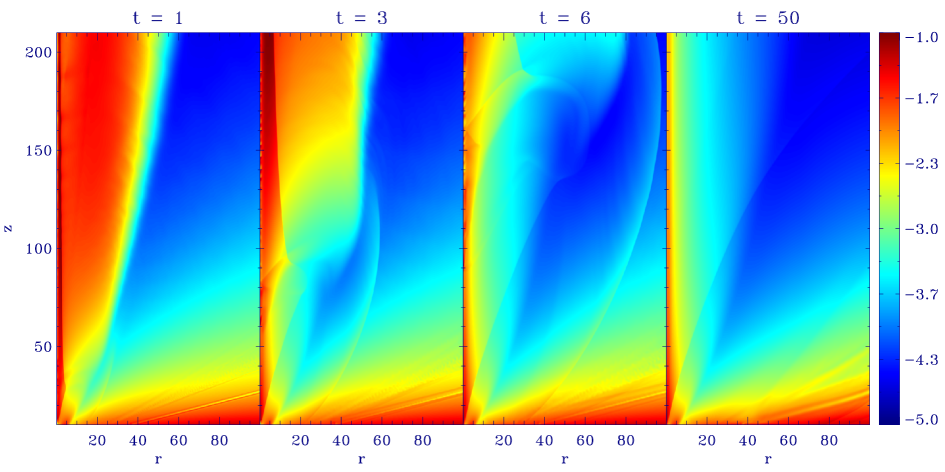
Figure 1: Logarithms of the density at different times for a typical model (5-q02). The time unit is $0.32\,$y (or $10$ Keplerian rotations of the footpoint of the matching surface). In the rightmost plot, a weak shock is observed along the diagonal. In addition, the initial matching surface, approximately at $r=5$ on the lower boundary, is still evident. To check this, compare it with the leftmost plot which describes a configuration very close to the initial one.

The logarithm of the density is plotted in Fig. 1 for different evolutionary stages of a typical two-component jet model (5-q02). The initial conditions correspond to equilibrium in the regions where each analytical solution dominates. However, around the matching surface, the models are modified and hence a strong perturbation is generated during the first timesteps of the simulation. An MHD wave propagates through the ADO solution without leaving behind any significant rearrangements. On the contrary, the equilibrium of the ASO model is substantially restructured, with its density dropping roughly by an order of magnitude. In only $\sim 100$ Keplerian rotations of the footpoint of the matching surface, the stellar component has already been totally and self consistently modified in the presence of the ADO solution.

From the rightmost plot of Fig. 1, notice that the initial matching surface is still evident. Indeed, this is expected, due to the fixed boundary conditions at the lower boundary. At $t=50$, the initial perturbation has almost left the domain, with the two-component jet having reached a steady state. Notice the formation of a weak steady shock, which can be seen almost along the diagonal direction of the computational domain.

Figure 2: The density fluctuations as a function of time calculated at the points $(r_{0}\,,z_{0})=(5\,,50)$, $(15\,,50)$ and $(30\,,50)$. The first is located in the ASO dominated region, the second close to the matching surface upstream of the shock and the third in the ADO dominated region (model 5-q02).

In order to establish the conclusion that the two components can co-exist in a steady state, we plot in Fig. 2 the density fluctuations for different time scales of three specific points. One is located inside the stellar component and the other two upstream of the shock, at the matching surface and in the disk wind, respectively. Evidently, for $t>2.5$ the solution remains almost unchanged up to $t=250$, i.e. a time longer by two orders of magnitude. The disk wind reaches the final exact equilibrium a bit later (at $t\sim 25$), due to the slower wave velocities of this region. Therefore, the rightmost plot of Fig. 1 represents a very well preserved steady state of the two intrinsically different jet components.

Both the physical and geometrical properties of the two winds are by definition considerably diverse, since their self-similar symmetries are orthogonal to each other. In turn, the same holds true for their respective poloidal critical surfaces. Therefore, the steady state of such a two-component jet was not a straightforward expectation. Nevertheless, it is clearly shown in Figs. 1 and 2 that the two complementary winds manage to co-exist. Also taking into account the artificial boundary effects present in long term simulations, investigated in Paper I, the above results are adequate to argue that the two-component jet models reach a well defined steady state.

Despite the fact that the plots concern a particular model, the same conclusions are valid for all the unperturbed scenarios presented in Table 2.

4.2 Deviations from the analytical solutions

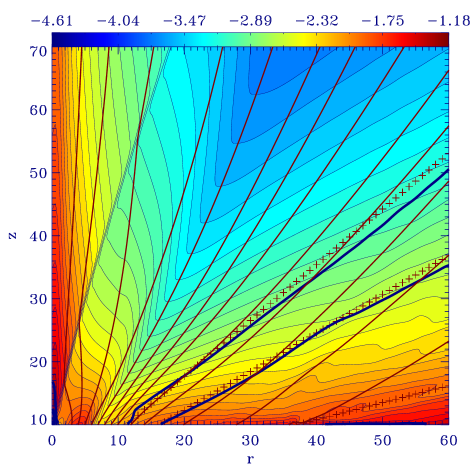
Figure 3: Logarithmic density contours (thin blue lines) for model 5-q02 at $t=50$. The magnetic poloidal fieldlines are overplotted with red lines. In the lower right part, going clockwise, the fast magnetosonic, the Alfvénic and the slow magnetosonic critical surfaces are plotted with red crosses for the ADO solution and with thick blue lines for the final numerical two-component flow.

Figure 4: The physical variables plotted at $z=50$ for the ADO model alone (solid line), the ASO model alone (dashed line), the initial setup of 5-q02 (diamonds) and its final configuration (crosses). The quantities displayed from left to right are: in the top row $\log\rho$, $\log P$ and $\log T$, in the middle row $V_{r}$, $V_{z}$ and $V_{\phi}$, in the bottom row $B_{r}$, $B_{z}$ and $B_{\phi}$.

Figure 5: The normalized integrals of motion plotted along three fieldlines of model 5-q02, rooted at the positions (from bottom to top) $(3\,,10)$, $(6\,,10)$, and $(9\,,10)$, corresponding to the ASO, mixing and ADO dominated regions, respectively. The distance from the lower boundary is parametrized by $s$.

Another crucial question that arises concerns how close the final outcome of the simulations is to the initial analytical solutions. In particular, the smaller the deviations are found to be, the more valid and robust are the analytical studies on the self-similar MHD outflows. This also implies the easy and appropriate extension of their conclusions to the two-component jet scenario, especially for the analytically derived disk winds.

Therefore, in Fig. 3 we plot the critical surfaces of the ADO solution (red crosses) and those of the final numerical two-component jet (thick blue lines), along with the logarithmic density contours and the magnetic fieldlines (red lines). The propagation of the perturbation described in §4.1 results in the slight modification of the fast magnetosonic and Alfvénic critical surface, as can be seen from their almost perfect match in Fig. 3. On the other hand, the slow magnetosonic critical surface seems to have collapsed towards the lower boundary. The slow waves generated initially at the matching surface by definition cannot pass to the sub slow domain. Consequently, if the surface stayed at its initial location, the waves would not have been able to leave the lower right region of the computational box. Such a phenomenon is observed in SC3 and SC5 runs of Stute et al. (Stu08 (2008)), where matter accumulates downstream of the slow critical surface. However, in our case, the separatrix is being bent downward, tangentially to the lower boundary, hence allowing the initial perturbation to exit the simulated box. As a result, the lower right region shows a significantly higher degree of deviation from the initial conditions than the rest of the domain. Nonetheless, it does reach a steady state asymptotically. Note that the critical surface cannot be dragged away, due to the fixed boundary conditions, which describe a sub slow flow at $z=10$. Similar features are also observed in Gracia et al. (Gra06 (2006)) and in most runs of Stute et al. (Stu08 (2008)).

The fact that the system finds an equilibrium so close to the analytical solution is due to the topological stability of the ADO model discussed in Paper I. No matter if the central part of the disk wind is substituted as a whole with a physically and geometrically different kind of outflow, the solution maintains all its properties, proving its stability.

The poloidal critical surfaces plotted in Fig. 3 also provide other insights into the two-component scenario. Close to the axis, they have an elliptical shape, as can be seen in the region very close to (0, 10), and eventually become conical, after the matching surface. Intuitively, this makes sense due to the difference in the symmetry of the accelerating mechanisms of the two winds. In Kwan et al. (Kwa07 (2007)), two types of outflows are observed, one emanating radially out of the protostar and the other being ejected at a constant angle with respect to the disk midplane. This implies a geometry of the poloidal critical surfaces similar to Fig. 3.

In Fig. 4, the physical variables are plotted at the constant height $z=50$, for the initial setup (diamonds) and final configuration (crosses) of model 5-q02. In addition, the initial ADO (solid lines) and ASO (dashed lines) solutions are also shown before their combination. All plots present the effect of the mixing function. Close to the axis, the ASO model dominates, whereas approaching the right boundary, the ADO becomes the main contributor. A jump can be observed in most quantities, which represents the weak shock discussed in §4.3. Apart from the density and the poloidal component of the magnetic field, the initial and final configurations converge at large distances, showing the stability of the ADO solution. However, this happens far from the slow magnetosonic critical surface. The modifications the initial ASO solution undergoes can be seen from the final equilibrium reached close to the axis. Note that the temperature plot can be used as a guide when looking for two-component jet parameters appropriate to address observed jets.

Finally, the normalized integrals of motion (Eqs. [5]-[9] of Paper I) are plotted in Fig. 5 along three selected fieldlines rooted at the points $(3\,,10)$, $(6\,,10)$, and $(9\,,10)$. One is in the ASO dominated part, one is in the ADO domain and the other is almost along the matching surface crossing the shock. In all cases the integrals are conserved with high accuracy, varying only within a few $\%$. At large distances from the shock, they tend to become constant, which indicates that the system reaches a steady state in all three regions. For the two inner fieldlines, at $s=5$ and $s=100$, respectively, the observed jumps are related to the crossing of the shock. In particular, the larger deviation from constancy occurs for the specific entropy integral $Q$, as expected.

4.3 Shock formation

Figure 6: Normalized discontinuities (from left to right) of the density, total pressure (thermal plus magnetic) and the entropy $Q$) across the shock, close to the point $(5\,,30)$. Notice that $s$ is increasing in the inverse direction of $r$.

Figure 7: A family of the characteristics (thin solid lines) of the fast magnetosonic waves in a zoomed super fast magnetosonic region around the shock (thick solid line) for model 5-q02. The thick dashed line is the initial matching surface.

In Fig. 6, we plot the normalized density, total pressure ($P+B^{2}/2$) and entropy $Q$ across the shock (direction right to left) around the position $(5\,,30)$, very close to the one assumed in Paper I. This point is located inside the domain where the stellar outflow dominates. Apparently, the density seems to increase by a factor of 2, whereas the pressure increases by a factor of 4. On the contrary, the jump seen in the entropy is very weak, being an order of magnitude smaller: this is not surprising, recalling that $\gamma=1.05$, i.e. conditions very close to isothermal, wherein entropy remains unchanged across shocks. Also there is no heating/cooling present in any simulation of this paper, thus making the above analysis simpler.

In Fig. 7 we plot one of the two families of the characteristics of the fast magnetosonic waves (thin lines) for model 5-q02, along with the initial matching surface (dashed line). It is evident that the shock (thick solid line) is not crossed by the downstream characteristics. This shows the causal disconnection of the two domains, upstream and downstream of the shock. In other words, the shock represents the horizon for the propagation of all MHD waves, coinciding with the numerical FMSS.

This feature is closely related to the ADO solution and was studied in detail in Paper I. However, the two-component case we present here is especially interesting for the following reason. The shock manifests even in the central area, where the contribution of the ASO model is total. This implies that it is not associated with the lower boundary, but on the contrary, it forms above it, intersecting the symmetry axis. Taking also into account the results of Paper I, the shock seems to be an intrinsic feature of the ADO solution. Consequently, the presence of the disk wind model in the two-component jet scenario has the remarkable characteristic of producing outflows that are causally disconnected to their launching region, despite the fact that the initial conditions causally connect the whole computational box.

4.4 Parameter study

In this section, we present the behavior of the two-component jets when we change the model parameters.

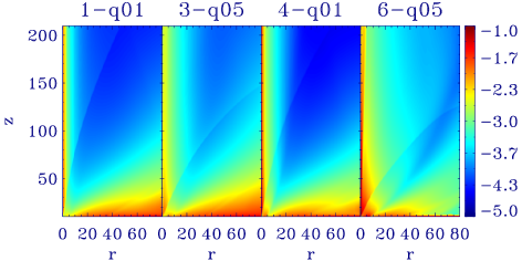
Figure 8: Logarithm of the density for the final numerical solutions of models 1-q01, 3-q05, 4-q01, 6-q05 (left to right). The two leftmost cases have a weaker stellar component compared to the two rightmost.

Fig. 8 shows the logarithm of the final density of the simulations carried out for models 1-q01, 3-q05, 4-q01, 6-q05 (left to right). When the position of the matching surface is rooted closer to the disk rather than the star, the shock seems to bend towards the midplane, confining the unmodified ADO solution in a smaller domain. This result indicates that as the spatial domination of the ASO solution becomes larger, the ADO model controls a smaller portion of the box, thus forming the shock closer to the disk.

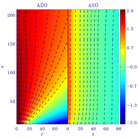
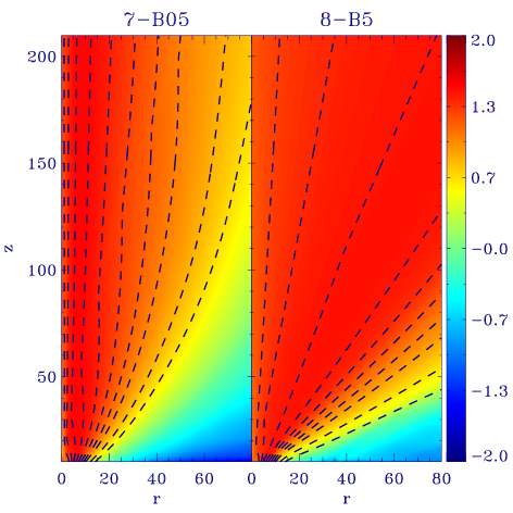
Figure 9: Logarithmic poloidal velocity and streamlines (dashed lines) for the unmixed ADO (top left) and ASO (top right) models separately. In the lower panel, models 7-B05 ($\ell_{B}=0.5$; left) and 8-B5 ($\ell_{B}=5$; right) are shown. The maximum values of the poloidal velocity of both of these two-component cases are $\sim 500\,$km s^-1, despite the misleading colorbar, which was accordingly chosen to match that of the top panel.

Recalling that models 1-q01 and 3-q05 have a weaker ASO contribution ($\ell_{B}=1$), compared to 4-q01 and 6-q05 ($\ell_{B}=2$), Fig. 8 also suggests that the relative strength of the ASO model does not seem to considerably affect the position of the shock, although larger deviations are seen around the slow critical surface of the initial ADO model. The same result is derived from models 7-B05, 8-B5 (bottom of Fig. 9) and 9-B10, where the location of the shock is found farther from the axis, the larger the value of $\ell_{B}$. Nevertheless, this might be related to the previous result since a large $\ell_{B}$ also spatially reduces the contribution coming from the ADO model.

Furthermore, Fig. 9 presents the logarithm of the poloidal velocity and the streamlines (dashed lines) for the ADO and ASO solutions separately, as well as for models 7-B05 ($\ell_{B}=0.5$) and 8-B5 ($\ell_{B}=5$). The left plot of the bottom panel suggests that for disk wind dominated jets, the ADO solution is effectively collimating the central component. However, we know that polytropically evolved ASO solutions become more collimated and less dense than the non polytropic initial ASO models (Paper I). So, it is rather difficult to disentangle the collimation due to the disk wind and that due to the change in energetics.

Moreover, increasing by one order of magnitude the contribution of the ASO model, the streamlines take an almost radial geometry (lower panel, right plot of Fig. 9). A similar result was obtained by Meliani et al. (Mel06 (2006)) when the mass loss rate of the inner stellar wind becomes comparable to the disk mass loss rate. Although this might contradict the parallel flow structure seen in the right plot of the top panel of Fig. 9, where the ASO solution is plotted alone, we note that such a strong collimation comes from the linear increase of $B_{\phi}$ (Fig. 4, dashed line). However, the two-component jet presents a more realistic distribution of current, with a decreasing toroidal field at large distances (Fig. 4, crosses) and hence the hoop stress is not capable of collimating the flow.

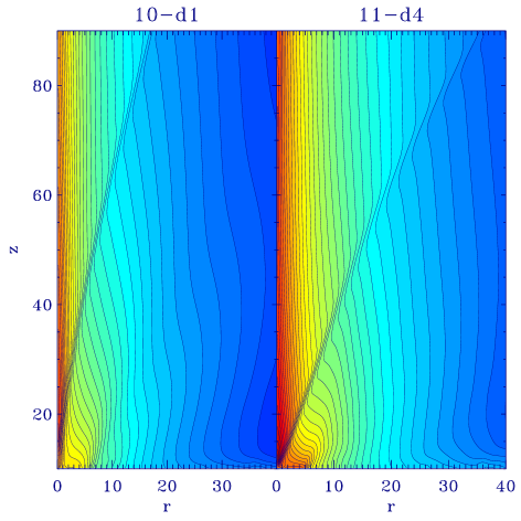
Figure 10: Logarithmic pressure contours for model 10-d1 on the left and 11-d4 on the right.

Finally, we examine how the third free parameter, $d$, which defines the steepness of the transition region, influences the final steady state reached by the two-component jets.

The pressure contours of models 10-d1 and 11-d4 shown in Fig. 10 suggest that no matter how smoothly the variables change from one solution to the other, the matching surface reaches the same sort of structure at the end of the simulations. On the other hand, the shock is affected more dramatically. In the $d=1$ case, it has a shape very similar to the one forming without the presence of the ASO solution (see Paper I), with a polar angle of $\sim 10^{\circ}$ as calculated close to the origin. On the contrary, the shock intersects the axis with a wider polar angle $\sim 15^{\circ}$ in the $d=4$ case. Note that although the value of the parameter may change inside the computational box, it is kept fixed at the lower boundary and hence influences the evolution.

4.5 Time variable stellar or X-type winds

This last section is dedicated to the stability issues raised by a potential time variability in the YSO’s outflow. We apply time dependency (Eq. [16] or [17]) either at the stellar wind’s base or around the X-point located at the interface between the stellar magnetosphere and the disk. The two-component jet parameters adopted are identical to model 5-q02.

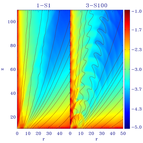
Figure 11: Magnetic fieldlines (red) and logarithmic density contours at $t=250$ for models 1-S1 (left) and 3-S100 (right).

High frequency velocity (or density) variations, associated with the Keplerian rotation at roughly a stellar radius, seem to fade away on larger scales, as shown on the left of Fig. 11. The structure remains very close to the unperturbed model. Two orders of magnitude lower frequency fluctuations, result in stronger gradients along the flow, as seen in the right panel of Fig. 11. Considering that the velocity varies by $\pm 50\%$ of its initial value, it is surprising how well the two-component jet structure is retained. Despite the “wiggling” of the magnetic field, the same flow features are found as in the unperturbed cases.

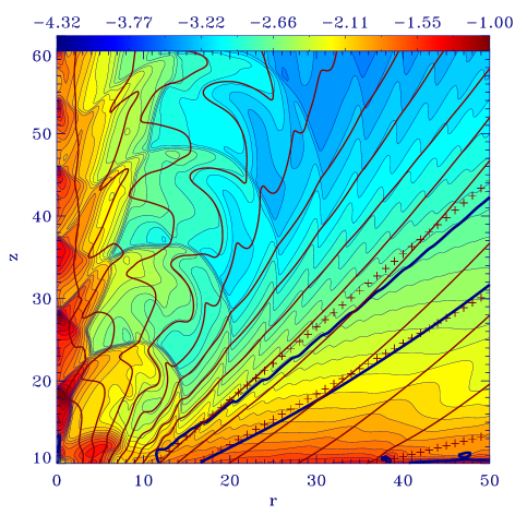
Figure 12: Logarithmic density contours (thin blue lines) and the magnetic field (red lines) for model 3-S10² at $t=50$. The red crosses and the thick blue lines denote the critical poloidal velocity surfaces of the ADO solution and those of the final equilibrium, respectively. This plot is equivalent to Fig. 3.

Fig. 12 displays a plot equivalent to Fig. 3 in order to understand how the shock and critical surfaces change in the time-variable stellar wind case. The picture is very similar, apart from the perturbations seen in the density throughout the computational box. The poloidal critical surfaces show the same behavior as in the unperturbed models and the weak steady shock is still present, being slightly curved locally as the fluctuations propagate.

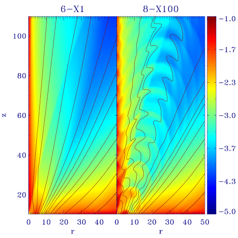
Figure 13: Logarithm of the density along with magnetic fieldlines (red lines) at $t=50$ for models 6-X1 and 8-X10².

Analogous results are derived by the models where time variability is enforced at the density and velocity of the outflow around the X-point. The momentum changes periodically by an order of magnitude. However, at the ASO and ADO dominated regions, the wind characteristics do not seem to be affected, especially in the high frequency variability case (model 6-X1, plot of left panel of Fig. 13). On the other hand, more evident structures are produced in the 100 times lower frequency fluctuations, still without destroying the basic pattern (model 8-X10², plot of right panel Fig. 13). This behaviour is similar to the stellar wind variability, but with a lesser degree of collimation.

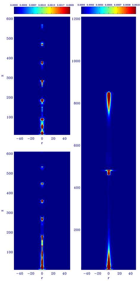
Figure 14: The quantity $\rho^{2}\sqrt{T}$, which is roughly related with emissivity, is plotted for the low frequency variability models examined in large scales. In the left, models 4a-S10³ (top) and 4b-S10³ (bottom) are shown, whereas in the right model 5-S10⁴ is displayed. Note that $\max(\rho^{2}\sqrt{T})=5.39\times 10^{-2}$ for model 4a-S10³, $\max(\rho^{2}\sqrt{T})=3.97\times 10^{-2}$ for model 4b-S10³ and $\max(\rho^{2}\sqrt{T})=7.49\times 10^{-3}$ for model 5-S10⁴. However, the colorbars use a lower maximum value in order to enhance the displayed features. The length code unit corresponds to $1\,$AU.

In order to see how the low frequency variability can affect the jet far away from the launching region, we plot the quantity $\rho^{2}\sqrt{T}$ for models 4a-S10³ (top left), 4b-S10³ (bottom left) and 5-S10⁴ (right) in Fig. 14. Close to the base, the numerical solutions remain close to the initial ADO and ASO models. However, at higher altitudes, the fluctuations create knot-like structures. It is evident that such models can be associated with some jet variability. We have checked that both stellar and X-wind type pulsations produce very similar structures far away from the disk-star system. This was expected, since kAU scales cannot distinguish the ejections coming from within $1\,$AU. The regular knot spacing observed in the jet of HH30 ($\sim 100\,$AU, Bacciotti et al. Bac99 (1999)) can be reasonably compared with our models 4a-S10³ and 4b-S10³, with a structure periodicity of $\sim 1\,$yr. Model 5-S10⁴, with a periodicity of $10\,$yrs, could be associated with the knots detected in the jet of HH34 where the condensation spacing is $\sim 1000\,$AU (Cohen & Jones Coh87 (1987)). Nevertheless, in this case there is a gap between the blobs and the star, suggesting a contribution of other processes to the knot formation. Note that the time scales of such fluctuations also correspond to typical stellar variabilities (e.g. the $11\,$y period of the solar cycle).

Figure 15: Density, pressure and sonic Mach number plotted along the jet axis for model 4a-S10³.

Finally, Fig. 15 provides the proof that these knot-like structures are in fact shocks. The top panel displays the periodic density and pressure jumps along the jet axis, with the change being approximately an order of magnitude for both. Note that close to the base the discontinuities are not yet well developed. We also remark that these shocks are stronger than that associated with the FMSS (see Fig. 6). The lower panel reports the sonic Mach number as a function of $z$. Its mean value of the background flow is $\sim 10$, in good accordance with YSO jet observations. The shocks propagate faster by $\sim 50\%$, as expected in agreement with the inflow time variability. Although Fig. 15 suggests that the flow values converge to a similar periodic structure, a larger computational box is needed to verify such an argument. In a future study, we plan to apply radiation cooling effects to these time variable models, effectively producing realistic emission maps to be compared to real data.

5 Summary and conclusions

In this work, we have constructed two-component numerical jet models by properly combining two well studied analytical solutions, each one describing separately a disk wind (ADO) and a stellar outflow (ASO). We have investigated the features of the time evolution and the characteristics of the final outcome of the simulations as a function of the two-component jet parameters and the enforced time variability. Although the detailed launching mechanisms of each component are not taken into account, the two-component jet models presented here seem able to capture the dynamics and describe a variety of interesting scenarios.

The main conclusions of this work are the following:

• The two-component jet models show remarkable stability and always reach a well defined steady state. This result is robust despite the fact that the two solutions have orthogonal symmetries, different geometry and different physics (i.e. launching mechanisms). In addition, the conclusion holds true independently of the choice of the parameters and even in the cases where time variability is enforced at the stellar wind’s base or around the X-point. Therefore, the analytical solutions provide solid foundations for realistic two-component jet scenarios.

• The system remains close to the initial analytical solutions. In particular, the disk wind dominated regions are barely changed in the presence of the stellar outflow, with the exception of the slow magnetosonic regions. On the other hand, the central component is self consistently modified due to the assumption of a polytropic equation of state and because of the effective collimation caused by the surrounding disk wind. This implies that specific YSO systems can be addressed more accurately by constructing analytical outflow solutions with the desirable characteristics, before merging them into a two-component regime.

• A shock manifests during the time evolution, preventing any information from the downstream domain from reaching the base of the outflow. This separatrix causally disconnects the two-component jet from its launching regions, although initially there is no such “horizon” present in the computational box. The initial ASO solution does not exhibit any modified fast separatrix (Sauty et al. Sau02 (2002)), whereas despite the existence of the FMSS in the initial ADO model (at small polar angles), it is effectively replaced by the stellar wind in the initial setup. Nonetheless, the final equilibria reached by the numerical models show the formation of a weak shock corresponding to such a surface, causally disconnecting the acceleration regions from the jet propagation physics and subsequent interaction with the outer medium.

• We may address various two-component jet scenarios, by means of two parameters controlling the relative contribution of each component, $\ell_{B}$, and the time variability function, $f(t)$. With the former, we can smoothly switch the physics from a totally magneto-centrifugal wind to a pressure driven jet. With the latter, flow fluctuations are introduced, producing knot-like structures on large scales that are quantitatively similar to HH30 and HH34 observations.

Thus, most of the technical part concerning two-component jets, e.g. 2.5D stability, steady states, parameter study, time variability etc., is now available, providing us with all the necessary ingredients to address YSO jets. With a) the proper analytical solutions, i.e. desirable lever arm, mass loss rate etc., b) the correct choice of the mixing parameters and c) an enforced time variability that effectively produces knot structures, we are now ready to qualitatively study different and realistic scenarios, address observed jet properties and ultimately understand the various outflow phases of specific T Tauri stars. However, such applications and comparison with relevant observational data is beyond the scope of this paper and will be presented in a future work.

Appendix A The self-similar outflow formulation

Axisymmetry, steady state and self-similarity assumptions simplify the ideal MHD equations to a set of coupled ODEs in spherical coordinates. These equations are solved numerically, providing the values of some key functions for each model.

For the ADO solution (radially self-similar), the physical variables are provided in terms of the tabulated key functions $G_{D}(\theta)$, $M_{D}(\theta)$ and $\psi_{D}(\theta)$:

$$\rho_{D}=\rho_{D*}\alpha_{D}^{x-3/2}\frac{1}{M_{D}^{2}}\,,\quad P_{D}=P_{D*}\alpha_{D}^{x-2}\frac{1}{M_{D}^{2\gamma}}\,,$$

$$\@vec{V}_{Dp}=-V_{D*}\alpha_{D}^{-1/4}\frac{M_{D}^{2}}{G_{D}^{2}}\frac{\sin\theta}{\cos(\psi_{D}+\theta)}\left(\cos\psi_{D}\hat{r}+\sin\psi_{D}\hat{z}\right)\,,$$

$$V_{D\phi}=V_{D*}\lambda\alpha_{D}^{-1/4}\frac{G_{D}^{2}-M_{D}^{2}}{G_{D}(1-M_{D}^{2})}\,,$$

$$\@vec{B}_{Dp}=-B_{D*}\alpha_{D}^{x/2-1}\frac{1}{G_{D}^{2}}\frac{\sin\theta}{\cos(\psi_{D}+\theta)}\left(\cos\psi_{D}\hat{r}+\sin\psi_{D}\hat{z}\right)\,,$$

$$B_{D\phi}=-B_{D*}\lambda\alpha_{D}^{x/2-1}\frac{1-G_{D}^{2}}{G_{D}(1-M_{D}^{2})}\,,$$

where $p$ denotes the poloidal component.

The ASO solution (meridionally self-similar) is described with the help of the key functions $G_{S}(R)$, $M_{S}(R)$, $F_{S}(R)$ and $\Pi_{S}(R)$:

$$\rho_{S}=\rho_{S*}\frac{1}{M_{S}^{2}}(1+\delta\alpha_{S})\,,\quad P_{S}=P_{S*}\Pi_{S}(1+\kappa\alpha_{S})\,,$$

$$V_{Sr}=V_{S*}\frac{M_{S}^{2}}{G_{S}^{2}}\frac{\sin\theta\cos\theta}{\sqrt{1+\delta\alpha_{S}}}\left(1-\frac{F_{S}}{2}\right)\,,$$

$$V_{Sz}=V_{S*}\frac{M_{S}^{2}}{G_{S}^{2}}\frac{1}{\sqrt{1+\delta\alpha_{S}}}\left(\cos^{2}\theta+\sin^{2}\theta\frac{F_{S}}{2}\right)\,,$$

$$V_{S\phi}=V_{S*}\lambda^{\prime}\alpha_{S}^{1/2}\frac{G_{S}^{2}-M_{S}^{2}}{G_{S}(1-M_{S}^{2})}\frac{1}{\sqrt{1+\delta\alpha_{S}}}\,,$$

$$B_{Sr}=B_{S*}\frac{\sin\theta\cos\theta}{G_{S}^{2}}\left(1-\frac{F_{S}}{2}\right)\,,$$

$$B_{Sz}=B_{S*}\frac{1}{G_{S}^{2}}\left(\cos^{2}\theta+\sin^{2}\theta\frac{F_{S}}{2}\right)\,,$$

$$B_{S\phi}=-B_{S*}\lambda^{\prime}\alpha_{S}^{1/2}\frac{1-G_{S}^{2}}{G_{S}(1-M_{S}^{2})}\,.$$