Darboux transformations for linear operators
on two dimensional regular lattices

Abstract.

Darboux transformations for linear operators on regular two dimensional lattices are reviewed. The six point scheme is considered as the master linear problem, whose various specifications, reductions, and their sublattice combinations lead to other linear operators together with the corresponding Darboux transformations. The second part of the review deals with multidimensional aspects of (basic reductions of) the four point scheme, as well as the three point scheme.

1. Introduction

Darboux transformations are a well known tool in the theory of integrable systems [72, 91, 48]. The classical Darboux transformation [15] deals with a Sturm–Liouville problem (the one dimensional stationary Schrödinger equation) generating, at the same time, new potentials and new wave functions from given ones thus providing solutions to the Korteweg–de Vries hierarchy of $1+1$ dimensional integrable systems. However, as it is clearly stated in [15], it was an earlier work of Moutard [74] which inspired Darboux. In that work one can find the proper transformation that applies to $2+1$ dimensional integrable systems. Note that the initial area of applications of the Darboux transformations, which preceded the theory of integrable systems, was the theory of conjugate and asymptotic nets where the large body of results on Darboux transformations was formulated [51, 15, 40, 104, 6, 63, 41].

Most of the techniques that allow us to find solutions of integrable non-linear differential equations have been successfully applied to difference equations. These include mutually interrelated methods such as bilinearization method [49] and the Sato approach [17, 19], direct linearization method [81, 80], inverse scattering method [1], the nonlocal $\bar{\partial}$ dressing method [10], the algebro-geometric techniques [59].

Also the method of the Darboux transformation has been successfully applied to the discrete integrable systems. The present paper aims to review application of the Darboux transformation technique for the equations that can be regarded as discretizations of second order linear differential equations in two dimensions (3.1), their distinguished subclasses and systems of such equations.

While presenting the results we are trying to keep the relation with continuous case. However, we are aware of weak points of this way of exposition. The theory of discrete integrable systems [103, 46] is reacher but also, in a sense, simpler then the corresponding theory of integrable partial differential equations. In the course of a limiting procedure, which gives differential systems from the discrete ones, various symmetries and relations between different discrete systems are lost. The classical example is provided (see, for example [11]) by the hierarchy of the Kadomsev–Petviashvilii (KP) equations, which can be obtained from a single Hirota–Miwa equation — the opposite way, from differential to discrete, involves all equations of the hierarchy [73].

The structure of the paper is as follows. In section 2 we expose main ideas in the theory of Darboux transformations in multidimension. In Section 3 we present the construction of the Darboux transformation for the discrete second order linear problem — the 6-point scheme (3.2) — which can be considered as a discretization of the general second order linear partial differential equation in two variables (3.1). Then we discuss various specifications and reductions of the 6-point scheme. We separately present in Section 3.4 the Darboux transformations for discrete self-adjoint two dimensional linear systems on the square, triangular and the honeycomb lattices, and their relation to the discrete Moutard transformation. Section 4 is devoted to detailed presentation of the Darboux transformations for systems of the 4-point linear problems, their various specifications and the corresponding permutability theorems. Section 5 is dedicated to reductions of the fundamental transformation compatible with additional restrictions on the form of the four point scheme. Finally, in Section 6 we review the Darboux transformations for the 3-point linear problem, and the corresponding celebrated Hirota’s discrete KP nonlinear system.

2. Jonas fundamental transformation and its basic reductions

The main idea included in the paper has its origin in Jonas paper [51] where fundamental transformation for conjugate nets has been presented. Neglecting the geometrical context of Jonas paper we only would like to say that the fundamental transformation acts on solutions of compatible system of second order linear differential equations on function $\psi:{\mathbb{R}}^{n}\to{\mathbb{R}}^{m}$

$$\psi,_{x^{i}x^{j}}=A^{ij}\psi,_{x^{i}}+A^{ji}\psi,_{x^{j}},\qquad i,j=1,...,n\qquad i\neq j$$

where coefficients $A^{ij}$ and $A^{ji}$ are functions of $(x^{i})$, and for $n>2$ they have to obey a nonlinear differential equation (compatibility conditions); we use notation that subscript preceded by coma denotes partial differentiation with respect to indicated variables.

Every fundamental transformation $\psi\mapsto\tilde{\psi}$ can be presented as composition of suitably chosen

1. radial transformation $\psi\mapsto\psi_{r}$

   $$\psi_{r}=\theta\psi$$

2. Combescure transformation $\psi_{r}\mapsto\tilde{\psi_{r}}$

   $${\tilde{\psi_{r}}},_{x^{i}}=\alpha_{i}{\psi_{r}},_{x^{i}}$$

3. radial transformation $\tilde{\psi_{r}}\mapsto\tilde{\psi}$

   $$\tilde{\psi}=\gamma\tilde{\psi_{r}}$$

We refer interested reader to Eisenhart book [40] for further details. As the practice shows the fundamental transformation is indeed fundamental - in the sense that most (if not all) of the Darboux transformations are reductions of the fundamental transformation.

Here we follow this basic idea discovered almost one hundred years ago. We start from presenting two dimensional difference operators $L$ (and corresponding difference equations $L\Psi=0$, where $\Psi$ is function of discrete variables $m$ and $n$) together with the transformation $(\Psi,L)\mapsto(\tilde{\Psi},\tilde{L})$ which is composition of

1. gauge transformation $(\Psi,L)\mapsto(\Psi_{r},L_{r})$ (see subsection 3.2)

   $$L_{r}=\Phi\circ L\circ\Theta,\qquad\Psi_{r}=\frac{\Psi}{\Theta}$$

   where $\Theta$ is a solution of $L\Theta=0$ whereas $\Phi$ is a solution of $L^{\dagger}\Phi=0$ where $L^{\dagger}$ denotes operator formally adjoint to operator $L$. We emphasize that this particular choice of functions $\Theta$ and $\Phi$ is essential, for it guarantees existence of function $\tilde{\Psi}_{r}$ in the next transformation

2. transformations $(\Psi_{r},L_{r})\mapsto(\tilde{\Psi}_{r},\tilde{L}_{r})$ that take either the form (details are given in the text below)

   (2.1) $$\begin{array}[]{l}\left[\begin{matrix}\Delta_{1}\tilde{\Psi}_{r}\cr\Delta_{2}\tilde{\Psi}_{r}\end{matrix}\right]=\left[\begin{matrix}\alpha&\beta\cr\gamma&\delta\end{matrix}\right]\left[\begin{matrix}\Delta_{1}\Psi_{r}\cr\Delta_{2}\Psi_{r}\end{matrix}\right]\end{array}$$

   or the form

   (2.2) $$\begin{array}[]{l}\left[\begin{matrix}\Delta_{1}\tilde{\Psi}_{r}\cr\Delta_{2}\tilde{\Psi}_{r}\end{matrix}\right]=\left[\begin{matrix}\alpha&\beta\cr\gamma&\delta\end{matrix}\right]\left[\begin{matrix}\Delta_{-1}\Psi_{r}\cr\Delta_{-2}\Psi_{r}\end{matrix}\right]\end{array}$$

   where $\Delta_{1}$, $\Delta_{2}$ denote forward difference operators $\Delta_{1}f(m,n):=f(m+1,n)-f(m,n)$, $\Delta_{2}f(m,n):=f(m,n+1)-f(m,n)$, whereas $\Delta_{-1}$, $\Delta_{-2}$ denote backward difference operators $\Delta_{-1}f(m,n):=f(m-1,n)-f(m,n)$, $\Delta_{-2}f(m,n):=f(m,n-1)-f(m,n)$.

3. gauge transformation $(\Psi_{r},L_{r})\mapsto(\tilde{\Psi}_{r},\tilde{L}_{r})$

   $$L_{r}=R\circ L\circ S,\qquad\Psi_{r}=\frac{\Psi}{S}$$

   where in general $R$ and $S$ are arbitrary functions (which should be specified when reductions or specifications of the transformations are considered).

Figure 1. Interrelations between schemes discussed in the text. The figure include: names of the schemes used in the text, position of the points the equation relates, numbers of sections where the DT for the scheme is discussed, the equation and its natural continuum limit (extensions of DT to multidimension are known only for the equations in rectangle frames)

We pay special attention to subclasses of operators $L$ that admit Darboux transformations. A trivial, from the point of view of integrable systems, examples are subclasses obtained by fixing a gauge (see section 3.2). Very important classes of operators are obtained by imposing conditions on the mentioned above functions $\Theta$ and $\Phi$. For example in the case of self-adjoint 7-point scheme we discuss in section 3.4.1, the relation is $\Phi=\Theta$. We refer to such procedures as to reductions. The further examples of reductions are given in sections 3.3.1, 3.3.2 and 5. We reserve separate name “specification” to the cases when the operator is reduced, whereas the transformations remain essentially unaltered (i.e. no constraint on functions $\Theta$ and $\Phi$ is necessary). Examples of specifications are given in sections 3.3, 3.4.2 and 3.5.

With the notion of “specification” another important issue appears, since continuous counterparts of the specifications presented here can be viewed as a choice of particular gauge and independent variables. The interesting (because not well understood) aspects of discrete integrable systems come from the fact there is no theory how to change discrete independent variables so that not to destroy underlying integrable phenomena. Sublattice approach, widely used in theoretical physics, can be regarded, to some extent, as counterpart of change of independent variables. To some extent, because the only case studied in detail from the point of view of Darboux transformations is the case of self-adjoint equation (3.29), which in the discrete case consists of Moutard case (section 3.3.2), self-adjoint case (section 3.4) and their mutual relations (c.f. [39, 38]). Interrelations between results presented here are summarized in Figure 1.

Large part of the paper is dedicated to the specification in which the matrix in (2.1) is diagonal. In this case one can consider systems of four point operators defined on lattices with arbitrary number of independent variables. The multidimensional lattices are extensively discussed in sections 4 and 5, where compact elegant expressions for superpositions of fundamental transformations are presented either.

3. Two dimensional systems

In this section we present discretizations of equation (3.1) and its subclasses covariant under Darboux transformations.

3.1. General case

Out of the schemes that can serve as a discretization of the 2D equation

(3.1) $$a\psi,_{xx}+b\psi,_{yy}+2c\psi,_{xy}+g\psi,_{x}+h\psi,_{y}=f\psi$$

the following 6-point scheme

(3.2) $$A\Psi_{(11)}+B\Psi_{(22)}+2C\Psi_{(12)}+G\Psi_{(1)}+H\Psi_{(2)}=F\Psi$$

deserve a special attention (coefficients $A$, $B$ etc. and dependent variable $\Psi$ are functions on ${\mathbb{Z}}^{2}$, subscript in brackets denote shift operators, $f(m,n)_{(1)}=f(m+1,n)$, $f(m,n)_{(2)}=f(m,n+1)$, $f(m,n)_{(11)}=f(m+2,n)$, $f(m,n)_{(22)}=f(m,n+2)$ and $f(m,n)_{(12)}=f(m+1,n+1)$). The scheme admits decomposition $[(\alpha_{1}T_{1}+\alpha_{2}T_{2}+\alpha_{3})(\beta_{1}T_{1}+\beta_{2}T_{2}+\beta_{3})+\gamma]\psi=0$ (where $T_{1}$ and $T_{2}$ are forward shift operators in first and second direction respectively) and therefore its Laplace transformations can be constructed (see [64, 15, 105, 20, 88, 2, 75] and Section 4.2.3 for the notion of the Laplace transformations of multidimensional linear operators). What more important from the point of view of this review the scheme is covariant under a fundamental Darboux transformation [76] (the transformation is often referred to as binary Darboux transformation in soliton literature). Indeed,

Theorem 3.1.

Given a non-vanishing solution $\Theta$ of (3.2)

(3.3) $$\begin{array}[]{l}A\Theta_{(11)}+B\Theta_{(22)}+2C\Theta_{(12)}+G\Theta_{(1)}+H\Theta_{(2)}=F\Theta\end{array}$$

and a non-vanishing solution $\Phi$ of the equation adjoint to equation (3.2)

(3.4) $$\begin{array}[]{l}A_{(-1-1)}\Phi_{(-1-1)}+B_{(-2-2)}\Phi_{(-2-2)}+2C_{(-1-2)}\Phi_{(-1-2)}+G_{(-1)}\Phi_{(-1)}+H_{(-2)}\Phi_{(-2)}=F\Phi\end{array}$$

(negative integers in brackets in subscript denote backward shift e.g. $f(m,n)_{(-1)}=f(m-1,n)$ etc.) the existence of auxiliary function $P$ is guaranteed

(3.5) $$\begin{array}[]{l}\Delta_{-1}(\Phi\Theta_{(12)}P)=B_{(-2)}\Phi_{(-2)}\Theta_{(2)}+B\Phi\Theta_{(22)}+C_{(-1)}\Phi_{(-1)}\Theta_{(2)}+C\Phi\Theta_{(12)}+H\Phi\Theta_{(2)}\\ \Delta_{-2}(\Phi\Theta_{(12)}P)=-(A_{(-1)}\Phi_{(-1)}\Theta_{(1)}+A\Phi\Theta_{(11)}+C_{(-2)}\Phi_{(-2)}\Theta_{(1)}+C\Phi\Theta_{(12)}+G\Phi\Theta_{(1)}).\end{array}$$

Then equation (3.2) can be rewritten as

(3.6) $$\begin{array}[]{l}\Delta_{2}\left[(C_{(-2)}+P_{(-2)})\Phi_{(-2)}\Theta_{(1)}\Delta_{1}\left(\frac{\Psi}{\Theta}\right)+B_{(-2)}\Phi_{(-2)}\Theta_{(2)}\Delta_{2}\left(\frac{\Psi}{\Theta}\right)\right]+\\ \Delta_{1}\left[A_{(-1)}\Phi_{(-1)}\Theta_{(1)}\Delta_{1}\left(\frac{\Psi}{\Theta}\right)-(P_{(-1)}-C_{(-1)})\Phi_{(-1)}\Theta_{(2)})\Delta_{2}\left(\frac{\Psi}{\Theta}\right)\right]=0\end{array}$$

which in turn guarantees the existence of functions $\Psi^{\prime}$ such that

(3.7) $$\begin{array}[]{l}\left[\begin{matrix}\Delta_{1}(\Psi^{\prime})\cr\Delta_{2}(\Psi^{\prime})\end{matrix}\right]=\left[\begin{matrix}(C_{(-2)}+P_{(-2)})\Phi_{(-2)}\Theta_{(1)}&B_{(-2)}\Phi_{(-2)}\Theta_{(2)}\cr-A_{(-1)}\Phi_{(-1)}\Theta_{(1)}&(P_{(-1)}-C_{(-1)})\Phi_{(-1)}\Theta_{(2)}\end{matrix}\right]\left[\begin{matrix}\Delta_{1}\left(\frac{\Psi}{\Theta}\right)\cr\Delta_{2}\left(\frac{\Psi}{\Theta}\right)\end{matrix}\right]\end{array}$$

Assuming that matrix in (3.7) is invertible on the whole lattice, i.e.
$D:=[(P_{(-1)}-C_{(-1)})(P_{(-2)}\!+\!C_{(-2)})+A_{(-1)}B_{(-2)}]\Theta_{(1)}\Theta_{(2)}\Phi_{(-1)}\Phi_{(-2)}\neq 0$ everywhere and finally on introducing $\tilde{\Psi}$ via

(3.8) $$\tilde{\Psi}=\frac{\Psi^{\prime}}{S}$$

and taking the opportunity of multiplying resulting equation by non-vanishing function $R$, we arrive at the conclusion that the function $\tilde{\Psi}$ satisfies equation of the form (3.2) but with new coefficients

(3.9) $$\begin{array}[]{l}\tilde{A}=\frac{RS_{(11)}\Phi\Theta_{(11)}}{D_{(1)}}A,\qquad\tilde{B}=\frac{RS_{(22)}\Phi\Theta_{(22)}}{D_{(2)}}B,\qquad\tilde{F}=\frac{RS\Phi\Theta}{D}F,\\ \\ \tilde{C}=\frac{RS_{(12)}}{2}\left(\frac{\Theta_{(11)}\Phi_{(1-2)}(C+P)_{(1-2)}}{D_{(1)}}+\frac{\Theta_{(22)}\Phi_{(-12)}(C-P)_{(-12)}}{D_{(2)}}\right),\\ \\ {\tilde{G}}=-{RS_{(1)}}\left(\frac{\Theta_{(11)}\Phi_{(1-2)}(C+P)_{(1-2)}+\Theta_{(11)}\Phi A}{D_{(1)}}+\frac{\Theta_{(2)}\Phi_{(-1)}(C-P)_{(-1)}+\Theta_{(1)}\Phi_{(-1)}A_{(-1)}}{D}\right),\\ \\ {\tilde{H}}=-{RS_{(2)}}\left(\frac{\Theta_{(22)}\Phi_{(-12)}(C-P)_{(-12)}+\Theta_{(22)}\Phi B}{D_{(2)}}+\frac{\Theta_{(1)}\Phi_{(-2)}(C+P)_{(-2)}+\Theta_{(2)}\Phi_{(-2)}B_{(-2)}}{D}\right),\end{array}$$

The family of maps $\Psi\mapsto\tilde{\Psi}$ given by (3.7)-(3.8) we refer to as Darboux transformations of equation (3.2).

3.2. Gauge equivalence

We say that two linear operators $L$ and $L^{\prime}$ are gauge equivalent if one can find functions say $\Phi$ and $\Theta$ such that $L^{\prime}=\Phi\circ L\circ\Theta$ (where $\circ$ stands for composition of operators). The idea to consider equivalence classes of linear operators (3.1) with respect to gauge rather than single operator itself, goes to Laplace and Darboux papers [64, 15]. In the continuous case it reflects in the fact that one can confine himself e.g. to equations (the so called affine gauge)

$$a\psi,_{xx}+b\psi,_{yy}+\psi,_{xy}+g\psi,_{x}+h\psi,_{y}=0$$

or to (in this case we would like to introduce the name basic gauge)

$$a\psi,_{xx}+b\psi,_{yy}+2c\psi,_{xy}+k,_{y}\psi,_{x}-k,_{x}\psi,_{y}=0$$

without loss of generality.

The Darboux transformation can be viewed as transformation acting on equivalence classes (with respect to gauge) of equation (3.2) (compare [76]). Therefore one can confine himself to particular elements of equivalence class. Commonly used choice is to confine oneself to the affine gauge i.e. to equations (3.2) that obeys

$$A+B+2C+G+H-F=0.$$

If one puts S = const in (3.8) (this condition is not necessary) then the above constraint is preserved under the Darboux transformation. One can consider further specification of the gauge

$$A+B+2C+G+H-F=0,\quad A_{(-12)}+B_{(1-2)}+2C+G_{(2)}+H_{(1)}-F_{(12)}=0$$

This choice of gauge we would like to refer as to basic gauge of equation (3.2). Note that if the equation (3.2) is in a basic gauge its formal adjoint is in a basic gauge too.

3.3. Specification to 4-point scheme and its reductions

In the continuous case due to possibility of changing independent variables one can reduce, provided equation (3.1) is hyperbolic, to canonical form

$$\psi,_{xy}+g\psi,_{x}+h\psi,_{y}=f\psi.$$

In the discrete case similar result can be obtained in a different way. Taking a glance at (3.9) we can notice that coefficients $A$, $B$ and $F$ transform in a very simple manner. In particular, if any of these coefficients equals zero then its transform equals zero too. Let us stress that in this case if we do so, we do not impose any constraints on transformation data, transformations remains essentially the same. First we shall concentrate on the case when two out of three mentioned functions vanish.

If we put

(3.10) $$A=0,\quad B=0,\quad C=\frac{1}{2}$$

then from equation (3.9)

$$\tilde{A}=0,\quad\tilde{B}=0$$

and one can adjust the function $R$ so that

$$\tilde{C}=\frac{1}{2}$$

so we arrive at the 4-point scheme

(3.11) $$\Psi_{(12)}=\alpha\Psi_{(1)}+\beta\Psi_{(2)}+\gamma\Psi.$$

and its fundamental transformation c.f. [10, 31, 71, 35].

We observe that the form of equation (3.11) is covariant under the gauge $L\mapsto\frac{1}{g_{(12)}}Lg$ and to identify whether two equations are equivalent or not we use the invariants of the gauge

(3.12) $$\kappa=\frac{\alpha_{(2)}\beta}{\gamma_{(2)}},\quad n=\frac{\alpha\beta_{(1)}}{\gamma_{(1)}}$$

Two equations are equivalent if their corresponding invariants $\kappa$ and $n$ are equal [75].

3.3.1. Goursat equation

In this subsection we discuss the discretization of class of equations

$$\psi,_{xy}=\frac{p,_{x}}{p}\psi,_{y}+p^{2}\psi$$

which is referred to as Goursat equation. The discrete counterpart of Goursat equation arose from the surveys on Egorov lattices [99] and symmetric lattices [32] and can be written in the form [75]

(3.13) $$\Psi_{(12)}=\frac{q_{(2)}}{q}\Psi_{(1)}+\Psi_{(2)}-\frac{\tau_{(12)}\tau}{\tau_{(1)}\tau_{(2)}}\frac{q_{(2)}}{q}\Psi$$

where functions $q$ and $\tau$ are related via

(3.14) $$q^{2}=\frac{\tau_{(1)}\tau_{(2)}-\tau_{(12)}\tau}{\tau^{2}_{(1)}}.$$

The gauge invariant characterization of the discrete Goursat equation is either

$$n_{(2)}^{2}=\kappa\kappa_{(12)}\frac{(1+\kappa_{(1)})(1+\kappa_{(2)})}{(1+\kappa)(1+\kappa_{(12)})}$$

or

$$\kappa_{(1)}^{2}=nn_{(12)}\frac{(1+n_{(1)})(1+n_{(2)})}{(1+n)(1+n_{(12)})}$$

The Goursat equation can be isolated from the others 4-point schemes in the similar way that Goursat did it over hundred years ago [45, 75] i.e. as the equation such that one of its Laplace transformations maps solutions of the equation to solutions of the adjoint equation. Therefore in this case if $\Theta$ obeys (3.13)

(3.15) $$\Theta_{(12)}=\frac{q_{(2)}}{q}\Theta_{(1)}+\Theta_{(2)}-\frac{\tau_{(12)}\tau}{\tau_{(1)}\tau_{(2)}}\frac{q_{(2)}}{q}\Theta$$

then its Laplace transformation

(3.16) $$\Phi=\frac{1}{q^{2}_{(2)}}\frac{\tau_{(2)}}{\tau_{(12)}}\Delta_{1}\Theta_{(2)}$$

is a solution of equation adjoint to equation (3.13) [75]. Equation (3.16) is the constraint we impose on transformation data (i.e. functions $\Theta$ and $\Phi$) in the fundamental transformation (3.7), (3.9) (we recall we have already put $A$ and $B$ equal to zero). In addition if $\Theta$ obeys (3.15) then

(3.17) $$\Delta_{1}\left(\frac{\tau}{\tau_{(2)}}\Theta^{2}\right)=\Delta_{2}\left[\frac{1}{q^{2}}\frac{\tau}{\tau_{(1)}}(\Delta_{1}\Theta)^{2}\right]$$

and as a result there exists function $\vartheta$ such that

(3.18) $$\Delta_{1}\vartheta=\frac{1}{q^{2}}\frac{\tau}{\tau_{(1)}}(\Delta_{1}\Theta)^{2},\quad\Delta_{2}\vartheta=\frac{\tau}{\tau_{(2)}}\Theta^{2}$$

Now it can be shown that one can put

(3.19) $$\Phi\Theta_{(12)}(P-\frac{1}{2})=-\vartheta_{(12)},\quad\Phi\Theta_{(12)}(P+\frac{1}{2})=\left[\sqrt{\frac{\tau_{(2)}}{\tau_{(1)}}}\frac{\sqrt{\Delta_{1}\vartheta\Delta_{2}\vartheta}}{q}\right]_{(2)}-\vartheta_{(2)}$$

and the transformation (3.7) takes form

(3.20) $$\begin{array}[]{l}\left[\begin{matrix}\Delta_{1}(\sqrt{\frac{{\tau}}{{\tau_{(2)}}}}\frac{\vartheta}{\sqrt{\Delta_{2}\vartheta}}\tilde{\Psi})\cr\Delta_{2}(\sqrt{\frac{{\tau}}{{\tau_{(2)}}}}\frac{\vartheta}{\sqrt{\Delta_{2}\vartheta}}\tilde{\Psi})\end{matrix}\right]=\left[\begin{matrix}\sqrt{\frac{\tau_{(2)}}{\tau_{(1)}}}\frac{\sqrt{\Delta_{1}\vartheta\Delta_{2}\vartheta}}{q}-\vartheta&0\cr 0&-\vartheta_{(2)}\end{matrix}\right]\left[\begin{matrix}\Delta_{1}\left(\sqrt{\frac{{\tau}}{{\tau_{(2)}}}}\frac{\Psi}{\sqrt{\Delta_{2}\vartheta}}\right)\cr\Delta_{2}\left(\sqrt{\frac{{\tau}}{{\tau_{(2)}}}}\frac{\Psi}{\sqrt{\Delta_{2}\vartheta}}\right)\end{matrix}\right]\end{array}$$

which is the discrete version of Goursat transformation [45]. The transformation rule for the field $\tau$ is

$$\tilde{\tau}=\tau\vartheta.$$

3.3.2. Moutard equation

In this subsection we discuss discretization Moutard equation and its (Moutard) transformation [74]

$$\psi,_{xy}=f\psi.$$

Moutard equation is self-adjoint equation (which allowed us to impose reduction $\Phi=\Theta$ in the continuous analogue of transformation (3.7) c.f. [76]). The point is that opposite to the continuous case there is no appropriate self-adjoint 4-point scheme

We do have the reduction of fundamental transformation that can be regarded as discrete counterpart of Moutard transformation. Namely, class of equations that can be written in the form

(3.21) $$\Psi_{(12)}+\Psi=M(\Psi_{(1)}+\Psi_{(2)})$$

we refer nowadays to as discrete Moutard equation. It appeared in the context of integrable systems in [19] and then its Moutard transformations have been studied in detail in [85]. Gauge invariant characterization of the class of discrete Moutard equations is [75]

$$n_{(2)}n=\kappa_{(1)}\kappa$$

Let us trace this reduction on the level of fundamental transformation. Putting $2C=-F$ and $G=H=:MF$ the equations (3.2), (3.3) and (3.4) take respectively form

(3.22) $$\begin{array}[]{l}F(\Psi_{(12)}+\Psi)=G(\Psi_{(1)}+\Psi_{(2)})\end{array}$$

(3.23) $$\begin{array}[]{l}F(\Theta_{(12)}+\Theta)=G(\Theta_{(1)}+\Theta_{(2)})\end{array}$$

(3.24) $$\begin{array}[]{l}F_{(-1-2)}\Phi_{(-1-2)}+F\Phi=G_{(-1)}\Phi_{(-1)}+G_{(-2)}\Phi_{(-2)}\end{array}$$

The crucial observation is: if the function $\Theta$ satisfies equation (3.23) then the function $\Phi$ given by

(3.25) $$\begin{array}[]{l}\Phi=\frac{1}{F}(\Theta_{(1)}+\Theta_{(2)})\end{array}$$

satisfies equation (3.24) [75]. If we put

$$2P=\frac{\Theta_{(1)}-\Theta_{(2)}}{\Phi}$$

then equations (3.5) will be automatically satisfied. If in addition we put in (3.8) $S=\Theta$ then Darboux transformation (3.7) takes form (c.f. [85])

(3.26) $$\left[\begin{matrix}\Delta_{1}(\Theta\tilde{\Psi})\cr\Delta_{2}(\Theta\tilde{\Psi})\end{matrix}\right]=\left[\begin{matrix}\Theta\Theta_{(1)}&0\cr 0&-\Theta\Theta_{(2)}\end{matrix}\right]\left[\begin{matrix}\Delta_{1}\frac{\Psi}{\Theta}\cr\Delta_{2}\frac{\Psi}{\Theta}\end{matrix}\right]$$

and it serves as transformation $\Psi\mapsto\tilde{\Psi}$ that maps solutions of equation (3.21) into solutions of another discrete Moutard equation

(3.27) $$\tilde{\Psi}_{(12)}+\tilde{\Psi}=\widetilde{M}(\tilde{\Psi}_{(1)}+\tilde{\Psi}_{(2)}),\quad\widetilde{M}=\frac{\Theta_{(1)}\Theta_{(2)}}{\Theta_{(12)}\Theta}M$$

We recall that $\Theta$ an arbitrary non-vanishing fixed solution of the equation (3.21)

(3.28) $$\Theta_{(12)}+\Theta=M(\Theta_{(1)}+\Theta_{(2)})$$

Every equation that is gauge equivalent to (3.24) we refer to as an adjoint discrete equation Moutard equation, its gauge invariant characterization is [75]

$$\kappa_{(12)}\kappa_{(1)}=n_{(12)}n_{(2)}.$$

Equation (3.23) can be regarded as potential version of equation (3.24)

3.4. Self-adjoint case

In the continuous case there is direct reduction of the fundamental transformation for equation (3.1) to the Moutard type transformation for self-adjoint equation [76]

(3.29) $$(a\psi,_{x}+c\psi,_{y}),_{x}+(b\psi,_{y}+c\psi,_{x}),_{y}=f\psi.$$

In this Section we present difference analogues of equation (3.29) which allow for the Darboux transformation.Opposite to the continuous case the transformation will not be direct reduction of the fundamental transformation for the 6-point scheme (3.2). The self-adjoint discrete operators studied below are however intimately related to discrete Moutard equation which provides the link between their Darboux transformations and the fundamental transformation for equation (3.1).

3.4.1. 7-point self-adjoint scheme

The following 7-point linear system

(3.30) $${\mathcal{A}}_{(1)}\Psi_{(1)}+{\mathcal{A}}\Psi_{(-1)}+{\mathcal{B}}_{(2)}\Psi_{(2)}+{\mathcal{B}}\Psi_{(-2)}+{\mathcal{C}}_{(1)}\Psi_{(1-2)}+{\mathcal{C}}_{(2)}\Psi_{(-12)}={\mathcal{F}}\Psi,$$

allows for the Darboux transformation [78].

Theorem 3.2.

Given scalar solution $\varTheta$ of the linear equation (3.30), then $\tilde{\Psi}$ given as solution of the following system

(3.31) $$\begin{pmatrix}\Delta_{1}(\tilde{\Psi}\varTheta)\\ \Delta_{2}(\tilde{\Psi}\varTheta)\end{pmatrix}=\begin{pmatrix}{\mathcal{C}}\varTheta_{(-1)}\varTheta_{(-2)}&-\varTheta_{(-2)}({\mathcal{B}}\varTheta+{\mathcal{C}}\varTheta_{(-1)})\\ \varTheta_{(-1)}\left({\mathcal{A}}\varTheta\!+\!{\mathcal{C}}\varTheta_{(-2)}\right)&-{\mathcal{C}}\varTheta_{(-1)}\varTheta_{(-2)}\end{pmatrix}\begin{pmatrix}\Delta_{-1}\frac{\Psi}{\varTheta}\\ \Delta_{-2}\frac{\Psi}{\varTheta}\end{pmatrix}$$

satisfies the 7-point scheme (3.30) with the new fields given by

(3.32) $$\tilde{{\mathcal{A}}}_{(1)}=\frac{\varTheta\varTheta_{(1)}{\mathcal{A}}}{\varTheta_{(-2)}{\mathcal{P}}},\qquad\tilde{{\mathcal{B}}}_{(2)}=\frac{\varTheta\varTheta_{(2)}{\mathcal{B}}}{\varTheta_{(-1)}{\mathcal{P}}},,\qquad\tilde{{\mathcal{C}}}=\frac{{\mathcal{C}}_{(-1-2)}\varTheta_{(-1)}\varTheta_{(-2)}}{\varTheta_{(-1-2)}{\mathcal{P}}_{(-1-2)}},$$

(3.33) $$\tilde{{F}}=\varTheta\left(\frac{\tilde{{\mathcal{A}}}_{(1)}}{\varTheta_{(1)}}+\frac{\tilde{{\mathcal{A}}}}{\varTheta_{(-1)}}+\frac{\tilde{{\mathcal{B}}}_{(2)}}{\varTheta_{(2)}}+\frac{\tilde{{\mathcal{B}}}}{\varTheta_{(-2)}}+\frac{\tilde{{\mathcal{C}}}_{(1)}}{\varTheta_{(1-2)}}+\frac{\tilde{{\mathcal{C}}}_{(2)}}{\varTheta_{(-12)}}\right)$$

where

(3.34) $${\mathcal{P}}=\varTheta{\mathcal{A}}{\mathcal{B}}+\varTheta_{(-1)}{\mathcal{C}}{\mathcal{A}}+\varTheta_{(-2)}{\mathcal{C}}{\mathcal{B}}.$$

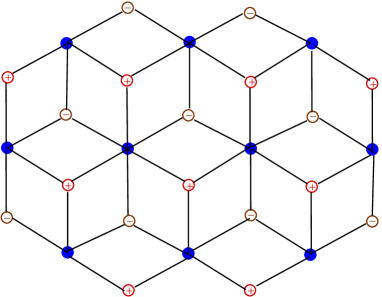
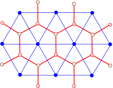
Figure 2. The bipartite quasi-regular rhombic tiling and the triangular and honeycomb lattices

As it was shown in [38] the self-adjoint 7-point scheme (3.30) can be obtained from the system of Moutard equations imposed consistently on quadrilaterals of the bipartite quasi-regular rhombic tiling (see Fig. 2), which is a particular case of the approach considered in [9]. Then the Moutard transformations can be also restricted to the triangular sublattice leading to Theorem 3.2.

3.4.2. Specification to 5-point scheme

The 7-point scheme admits specification ${\mathcal{C}}=0$ (alternatively one can put ${\mathcal{A}}=0$ or ${\mathcal{B}}=0$) and as result we obtain specification to 5-point self-adjoint scheme [78].

(3.35) $${\mathcal{A}}_{(1)}\Psi_{(1)}+{\mathcal{A}}\Psi_{(-1)}+{\mathcal{B}}_{(2)}\Psi_{(2)}+{\mathcal{B}}\Psi_{(-2)}={\mathcal{F}}\Psi.$$

The self-adjoint 5-point scheme and its Darboux transformation can be also obtained form the Moutard equation on the (bipartite) square lattice [39].

3.4.3. The honeycomb lattice

It is well known that the triangular and honeycomb grids are dual to each other (see Fig. 2). Restriction of the system of the Moutard equations on the rhombic tiling to the honeycomb sublattice gives [38] the following linear system

(3.36) $$\frac{1}{{\mathcal{A}}}(\Psi^{+}-\Psi^{-})+\frac{1}{{\mathcal{B}}}(\Psi^{+}_{(-12)}-\Psi^{-})+\frac{1}{{\mathcal{C}}_{(12)}}(\Psi^{+}_{(2)}-\Psi^{-}) =0,$$

(3.37) $$\frac{1}{{\mathcal{A}}}(\Psi^{-}-\Psi^{+})+\frac{1}{{\mathcal{B}}_{(1-2)}}(\Psi^{-}_{(1-2)}-\Psi^{+})+\frac{1}{{\mathcal{C}}_{(1)}}(\Psi^{-}_{(-2)}-\Psi^{+}) =0.$$

Remark.

Because $\Psi^{-}$ and $\Psi^{+}$ satisfy separately the self-adjoint 7-point schemes (3.30), but with different coefficients, then the linear problem (3.36)-(3.37) can be considered as a relation between two equations (3.30). This is the Laplace transformation between self-adjoint 7-point schemes studied in [88, 87].

The corresponding restriction of the Moutard transformation gives the Darboux transformation for the honeycomb linear problem.

Theorem 3.3.

Given scalar solution $(\varTheta^{+},\varTheta^{-})$ of the honeycomb linear system (3.36)-(3.37) then the solution $(\tilde{\Psi}^{+},\tilde{\Psi}^{-})$ of the system

(3.38) $$\tilde{\Psi}^{+}_{(2)}-\tilde{\Psi}^{-} =\frac{{\mathcal{C}}}{{\mathcal{R}}}\left(\varTheta^{-}_{(-2)}\Psi^{-}_{(-1)}-\theta^{-}_{(-1)}\Psi^{-}_{(-2)}\right),$$

(3.39) $$\tilde{\Psi}^{+}-\tilde{\Psi}^{-} =\frac{{\mathcal{A}}_{(-1)}}{{\mathcal{R}}}\left(\varTheta^{-}_{(-1-2)}\Psi^{-}_{(-2)}-\varTheta^{-}_{(-2)}\Psi^{-}_{(-1-2)}\right),$$

(3.40) $$\tilde{\Psi}^{-}-\tilde{\Psi}^{+}_{(-12)} =\frac{{\mathcal{B}}_{(-2)}}{{\mathcal{R}}}\left(\varTheta^{-}_{(-1-2)}\Psi^{-}_{(-1)}-\varTheta^{-}_{(-1)}\Psi^{-}_{(-1-2)}\right),$$

with ${\mathcal{R}}$ given by

(3.41) $${\mathcal{R}}={\mathcal{A}}_{(-1)}{\mathcal{B}}_{(-2)}+{\mathcal{C}}{\mathcal{A}}_{(-1)}+{\mathcal{C}}{\mathcal{B}}_{(-2)},$$

satisfies a new honeycomb linear system with the coefficients

(3.42) $$\tilde{\mathcal{A}}=\frac{{\mathcal{A}}_{(-1)}}{{\mathcal{R}}}\varTheta^{-}_{(-2)}\varTheta^{-}_{(-1-2)},\qquad\tilde{\mathcal{B}}=\frac{{\mathcal{B}}_{(-2)}}{{\mathcal{R}}}\varTheta^{-}_{(-1)}\varTheta^{-}_{(-1-2)},\qquad\tilde{\mathcal{C}}_{(12)}=\frac{{\mathcal{C}}}{{\mathcal{R}}}\varTheta^{-}_{(-1)}\varTheta^{-}_{(-2)}.$$

3.5. Specification to 3-point scheme

We end the review of two-dimensional case with specification to the 3-point scheme i.e. to a discretization of first order differential equation

$$g\psi,_{x}+h\psi,_{y}=f\psi.$$

If we put

$$A=0,\quad B=0,\quad F=0$$

then according to (3.9)

$$\tilde{A}=0,\quad\tilde{B}=0,\quad\tilde{F}=0$$

It means that the fundamental transformation (3.7) is also the Darboux transformation for the 3-point scheme [18, 82]

$$2C\Psi_{(12)}+G\Psi_{(1)}+H\Psi_{(2)}=0.$$

This elementary scheme is the simplest one from the class considered here, but it deserves a special attention, because it leads to one of the most studied integrable discrete equation [49]. We confine ourselves to recalling briefly in Section 6 main results in this field.

To the end let us rewrite the 3-point scheme in the basic gauge

(3.43) $$(u_{(2)}-u_{(1)})\Psi_{(12)}+(u_{(1)}-u)\Psi_{(1)}-(u_{(2)}-u)\Psi_{(2)}=0$$

4. The four point systems

In this Section we present the Darboux transformations for the four point scheme (the discrete Laplace equation) from the point of view of systems of such equations, and the corresponding permutability theorems. To keep the paper of reasonable size and in order to present the results from a simple algebraic perspective we do not discuss important relations of the subject to incidence and difference geometry [20, 31, 7, 13, 21, 25, 26, 27, 35, 32, 54, 55, 57, 58, 100, 101, 39, 38] (see also [33, 8] and earlier works [97, 98]), application of analytic [10, 34, 35, 37, 107, 106, 108, 36, 32, 70, 29] and algebro-geometric [59, 60, 4, 22, 23, 5, 39, 26, 47, 27] techniques of the integrable systems theory to construct large classes of solutions of the linear systems in question and solutions of the corresponding nonlinear discrete equations.

In order to simplify discussion of the Darboux transformations for systems of the 4-point schemes we fix (without loss of generality [31]) the gauge to the affine one

(4.1) $$\boldsymbol{\Psi}_{(ij)}=A_{ij(i)}\boldsymbol{\Psi}_{(i)}+A_{ji(j)}\boldsymbol{\Psi}_{(j)}+(1-A_{ij(i)}-A_{ji(j)})\boldsymbol{\Psi},\qquad i\neq j,$$

where $A_{ij}:{\mathbb{Z}}^{N}\to{\mathbb{R}}$ are some functions constrained by the compatibility of the system (4.1). It is also convenient [10] to replace the second order linear system (4.1) by a first order system as follows. The compatibility of (4.1) allows for definition of the potentials (the Lamé coefficients) $H_{i}:{\mathbb{Z}}^{N}\to{\mathbb{R}}$ such that

(4.2) $$A_{ij}=\frac{H_{i(j)}}{H_{i}},\;\;\;i\neq j\;.$$

The new wave functions $\boldsymbol{\psi}_{i}$ given by the decomposition

(4.3) $${\Delta}_{i}\boldsymbol{\Psi}=H_{i(i)}\boldsymbol{\psi}_{i}\;,$$

satisfy the first order linear system

(4.4) $$\Delta_{j}\boldsymbol{\psi}_{i}=Q_{ij(j)}\boldsymbol{\psi}_{j},\;\;\;i\neq j\;,$$

where the functions $Q_{ij}$, called the rotation coefficients, are calculated from the equation

(4.5) $${\Delta}_{i}H_{j}=Q_{ij}H_{i(i)},\;\;\;i\neq j\;,$$

which is called adjoint to (4.4). Both the equations (4.5) and (4.4) are compatible provided the fields $Q_{ij}$ satisfy the discrete Darboux equations [10]

(4.6) $${\Delta}_{k}Q_{ij}=Q_{ik(k)}Q_{kj}\;\;,\qquad i\neq j\neq k\neq i.$$

Corollary 4.1.

Due to (4.4) the function $\boldsymbol{\psi}_{i}$ satisfies itself the four point equation

(4.7) $$\boldsymbol{\psi}_{i(ij)}=\boldsymbol{\psi}_{i(i)}+\frac{Q_{ij(ij)}}{Q_{ij(j)}}\boldsymbol{\psi}_{i(j)}-\frac{Q_{ij(ij)}}{Q_{ij(j)}}\left(1-Q_{ij(j)}Q_{ji(i)}\right)\boldsymbol{\psi}_{i},\qquad i\neq j,$$

while the function $\left(\frac{H_{j}}{Q_{ij}}\right)_{(ij)}$ satifies the adjoint of (4.7) in the sense of (3.4).

The discrete Darboux equations imply existence of the potentials $\rho_{i}$ given as solutions of the compatible system

(4.8) $$\frac{\rho_{i(j)}}{\rho_{i}}=1-Q_{ji(i)}Q_{ij(j)},\qquad i\neq j\;,$$

and yet another potential $\tau$ such that

(4.9) $$\rho_{i}=\frac{\tau_{(i)}}{\tau}.$$

In terms of the $\tau$-function and the functions

(4.10) $$\tau_{ij}=\tau Q_{ij}\;,$$

the meaning of which will be given in section 4.2.3, equations (4.8) and (4.6) can be rewritten [37, 32] in the bilinear form

(4.11) $$\tau_{(ij)}\tau =\tau_{(i)}\tau_{(j)}-\tau_{ji(i)}\tau_{ij(j)}\;,\qquad i\neq j$$

(4.12) $$\tau_{ij(k)}\tau =\tau_{(k)}\tau_{ij}+\tau_{ik(k)}\tau_{kj}\;,\qquad i\neq j\neq k\neq i.$$

4.1. The vectorial fundamental (bilinear Darboux) transformation

We start with a simple algebraic fact, whose consequences will be discussed throughout the remaining part of this Section.

Theorem 4.2 ([71]).

Given the solution $\boldsymbol{\phi}_{i}:\mathbb{Z}^{N}\to{\mathbb{U}}$, of the linear system (4.4), and given the solution $\boldsymbol{\phi}^{*}_{i}:\mathbb{Z}^{N}\to{\mathbb{W}}^{*}$, of the adjoint linear system (4.5). These allow to construct the linear operator valued potential $\boldsymbol{\Omega}[\boldsymbol{\phi},\boldsymbol{\phi}^{*}]:\mathbb{Z}^{N}\to\mathrm{L}({\mathbb{W}},{\mathbb{U}})$, defined by

(4.13) $$\Delta_{i}\boldsymbol{\Omega}[\boldsymbol{\phi},\boldsymbol{\phi}^{*}]=\boldsymbol{\phi}_{i}\otimes\boldsymbol{\phi}^{*}_{i(i)},\qquad i=1,\dots,N.$$

If ${\mathbb{W}}={\mathbb{U}}$ and the potential $\boldsymbol{\Omega}$ is invertible, $\boldsymbol{\Omega}[\boldsymbol{\phi},\boldsymbol{\phi}^{*}]\in\mathrm{GL}({\mathbb{W}})$, then

(4.14) $$\tilde{\boldsymbol{\phi}}_{i} =\boldsymbol{\Omega}[\boldsymbol{\phi},\boldsymbol{\phi}^{*}]^{-1}\boldsymbol{\phi}_{i},\;\;\;i=1,...,N,$$

(4.15) $$\tilde{\boldsymbol{\phi}}^{*}_{i} =\boldsymbol{\phi}^{*}_{i}\boldsymbol{\Omega}[\boldsymbol{\phi},\boldsymbol{\phi}^{*}]^{-1},\;\;\;i=1,...,N,$$

satisfy the linear systems (4.4)-(4.5) correspondingly, with the fields

(4.16) $$\tilde{Q}_{ij}=Q_{ij}-\langle\boldsymbol{\phi}^{*}_{j}|\boldsymbol{\Omega}[\boldsymbol{\phi},\boldsymbol{\phi}^{*}]^{-1}|\boldsymbol{\phi}_{i}\rangle,\;\;\;i,j=1,\dots,N,\;\;i\neq j,.$$

In addition,

(4.17) $$\boldsymbol{\Omega}[\tilde{\boldsymbol{\phi}},\tilde{\boldsymbol{\phi}}^{*}]=C-\boldsymbol{\Omega}[\boldsymbol{\phi},\boldsymbol{\phi}^{*}]^{-1},$$

where $C$ is a constant operator.

Remark.

Notice that because of (4.3) we have $\Psi=\boldsymbol{\Omega}[\boldsymbol{\psi},H]$.

Corollary 4.3 ([69]).

The potentials $\rho_{i}$ and the $\tau$-function transform according to

(4.18) $$\tilde{\rho}_{i} =\rho_{i}(1+\boldsymbol{\phi}^{*}_{i(i)}\boldsymbol{\Omega}[\boldsymbol{\phi},\boldsymbol{\phi}^{*}]^{-1}\boldsymbol{\phi}_{i}),$$

(4.19) $$\tilde{\tau} =\tau\det\boldsymbol{\Omega}[\boldsymbol{\phi},\boldsymbol{\phi}^{*}].$$

Applying the above transformation one can produce new compatible (affine) four point linear problems from the old ones.

To obtain conventional transformation formulas consider [35] the following splitting of the vector space ${\mathbb{W}}$ of Theorem 4.2:

(4.20) $${\mathbb{W}}={\mathbb{E}}\oplus{\mathbb{V}}\oplus{\mathbb{F}}\;,\;\;\;{\mathbb{W}}^{*}={\mathbb{E}}^{*}\oplus{\mathbb{V}}^{*}\oplus{\mathbb{F}}^{*}\;\;\;\;,$$

if

(4.21) $$\boldsymbol{\phi}_{i}=\begin{pmatrix}\boldsymbol{\psi}_{i}\\ \boldsymbol{\theta}_{i}\\ 0\end{pmatrix},\;\;\;\boldsymbol{\phi}^{*}_{i}=(0,\boldsymbol{\theta}^{*}_{i},\boldsymbol{\psi}^{*}_{i})\;,$$

then, the corresponding potential matrix is of the form

(4.22) $$\boldsymbol{\Omega}[\boldsymbol{\phi},\boldsymbol{\phi}^{*}]=\begin{pmatrix}{\mathbb{I}}_{\mathbb{E}}&\boldsymbol{\Omega}[\boldsymbol{\psi},\boldsymbol{\theta}^{*}]&\boldsymbol{\Omega}[\boldsymbol{\psi},\boldsymbol{\psi}^{*}]\\ 0&\boldsymbol{\Omega}[\boldsymbol{\theta},\boldsymbol{\theta}^{*}]&\boldsymbol{\Omega}[\boldsymbol{\theta},\boldsymbol{\psi}^{*}]\\ 0&0&{\mathbb{I}}_{\mathbb{F}}\end{pmatrix}$$

and its inverse is

(4.23) $$\boldsymbol{\Omega}[\boldsymbol{\phi},\boldsymbol{\phi}^{*}]^{-1}=\begin{pmatrix}{\mathbb{I}}_{\mathbb{E}}&-\boldsymbol{\Omega}[\boldsymbol{\psi},\boldsymbol{\theta}^{*}]\boldsymbol{\Omega}[\boldsymbol{\theta},\boldsymbol{\theta}^{*}]^{-1}&-\boldsymbol{\Omega}[\boldsymbol{\psi},\boldsymbol{\psi}^{*}]+\boldsymbol{\Omega}[\boldsymbol{\psi},\boldsymbol{\theta}^{*}]\boldsymbol{\Omega}[\boldsymbol{\theta},\boldsymbol{\theta}^{*}]^{-1}\boldsymbol{\Omega}[\boldsymbol{\theta},\boldsymbol{\psi}^{*}]\\ 0&\boldsymbol{\Omega}[\boldsymbol{\theta},\boldsymbol{\theta}^{*}]^{-1}&-\boldsymbol{\Omega}[\boldsymbol{\theta},\boldsymbol{\theta}^{*}]^{-1}\boldsymbol{\Omega}[\boldsymbol{\theta},\boldsymbol{\psi}^{*}]\\ 0&0&{\mathbb{I}}_{\mathbb{F}}\end{pmatrix}.$$

Let us consider the case of $K$-dimensional transformation data space, ${\mathbb{V}}={\mathbb{R}}^{K}$, and ${\mathbb{F}}={\mathbb{R}}$, ${\mathbb{E}}={\mathbb{R}}^{M}$, then the transformed solution $\tilde{\boldsymbol{\Psi}}=\boldsymbol{\Omega}[\tilde{\boldsymbol{\psi}},\tilde{H}]$ of the four point scheme (recall that $\boldsymbol{\Psi}=\boldsymbol{\Omega}[\boldsymbol{\psi},H]$) up to a constant vector reads

(4.24) $$\tilde{\boldsymbol{\Psi}}=\boldsymbol{\Psi}-\boldsymbol{\Omega}[\boldsymbol{\psi},\boldsymbol{\theta}^{*}]\boldsymbol{\Omega}[\boldsymbol{\theta},\boldsymbol{\theta}^{*}]^{-1}\boldsymbol{\Omega}[\boldsymbol{\theta},H],$$

where the corresponding transformed solutions $\tilde{\boldsymbol{\psi}}_{i}$ of the linear problem (4.4) and $\tilde{H}_{i}$ of the adjoint linear problem (4.5) are given by equations

(4.25) $$\tilde{\boldsymbol{\psi}}_{i} =\boldsymbol{\psi}_{i}-\boldsymbol{\Omega}[\boldsymbol{\psi},\boldsymbol{\theta}^{*}]\boldsymbol{\Omega}[\boldsymbol{\theta},\boldsymbol{\theta}^{*}]^{-1}\boldsymbol{\theta}_{i},$$

(4.26) $$\tilde{H}_{i} =H_{i}-\boldsymbol{\theta}^{*}_{i}\boldsymbol{\Omega}[\boldsymbol{\theta},\boldsymbol{\theta}^{*}]^{-1}\boldsymbol{\Omega}[\boldsymbol{\theta},H],$$

and

(4.27) $$\tilde{Q}_{ij}=Q_{ij}-\boldsymbol{\theta}^{*}_{j}\boldsymbol{\Omega}[\boldsymbol{\theta},\boldsymbol{\theta}^{*}]^{-1}\boldsymbol{\theta}_{i}.$$

The scalar ($K=1$) fundamental transformation in the above form was given in [57].

Remark.

To connect the above formalism to the results of Section 3 notice that given scalar solution $\theta_{i}$ of the linear system (4.4) then the potential $\Theta=\Omega[\theta,H]$ is the scalar solution of the system (4.1) of second order linear equations. Moreover, given the solution $\theta^{*}_{i}$, of the adjoint linear system (4.5) then the functions

(4.28) $$\sigma_{i}=\frac{\theta^{*}_{i}}{H_{i}}$$

satisfy [35] the linear system

(4.29) $$\Delta_{j}\sigma_{i}=(A_{ij}-1)\left(\sigma_{j(j)}-\sigma_{i(j)}\right),\qquad i\neq j.$$

Equations (4.29) imply that the functions

(4.30) $$\Phi_{ij}=\sigma_{i(ij)}-\sigma_{j(ij)},\qquad i\neq j,$$

satisfy the corresponding equations

(4.31) $$\Phi_{ij(-i-j)}=A_{ij}\Phi_{ij(-i)}+A_{ji}\Phi_{ij(-j)}+(1-A_{ij(i)}-A_{ji(j)})\Phi_{ij},\qquad i\neq j,$$

adjoint of equations (4.1). In the case $M=2$ we obtain therefore the data of the transformation being the solution $\Theta$ of the linear problem and the solution $\Phi=\Phi_{12}$ of its adjoint, thus we recover results of Theorem 3.1 with the four point specification (3.10) in the affine gauge; see [25] for more detailed description. Notice that in order to describe fundamental transformation in the second order formalism for $M>2$ one should consider in addition the algebraic relations

$$\Phi_{ij}=-\Phi_{ji},\qquad\Phi_{ij(-i-j)}+\Phi_{jk(-j-k)}=\Phi_{ik(-i-k)},$$

which are consequences of definition (4.30).

It is important to notice that the vectorial fundamental transformation can be obtained as a superposition of $K$ scalar transformations, which follows from the following observation.

Proposition 4.4 ([35]).

Assume the following splitting of the data of the vectorial fundamental transformation

(4.32) $$\boldsymbol{\theta}_{i}=\left(\begin{array}[]{c}\boldsymbol{\theta}_{i}^{a}\\ \boldsymbol{\theta}_{i}^{b}\end{array}\right),\qquad\boldsymbol{\theta}_{i}^{*}=\left(\begin{array}[]{cc}\boldsymbol{\theta}_{ai}^{*}&\boldsymbol{\theta}_{bi}^{*}\end{array}\right),$$

associated with the partition ${\mathbb{R}}^{K}={\mathbb{R}}^{K_{a}}\oplus{\mathbb{R}}^{K_{b}}$, which implies the following splitting of the potentials

(4.33) $$\boldsymbol{\Omega}[\boldsymbol{\theta},H]=\left(\begin{array}[]{c}\boldsymbol{\Omega}[\boldsymbol{\theta}^{a},H]\\ \boldsymbol{\Omega}[\boldsymbol{\theta}^{b},H]\end{array}\right),\qquad\boldsymbol{\Omega}[\boldsymbol{\theta},\boldsymbol{\theta}^{*}]=\left(\begin{array}[]{cc}\boldsymbol{\Omega}[\boldsymbol{\theta}^{a},\boldsymbol{\theta}_{a}^{*}]&\boldsymbol{\Omega}[\boldsymbol{\theta}^{a},\boldsymbol{\theta}_{b}^{*}]\\ \boldsymbol{\Omega}[\boldsymbol{\theta}^{b},\boldsymbol{\theta}_{a}^{*}]&\boldsymbol{\Omega}[\boldsymbol{\theta}^{b},\boldsymbol{\theta}_{b}^{*}]\end{array}\right),$$

(4.34) $$\boldsymbol{\Omega}[\boldsymbol{\psi},\boldsymbol{\theta}^{*}]=\left(\begin{array}[]{cc}\boldsymbol{\Omega}[\boldsymbol{\psi},\boldsymbol{\theta}_{a}^{*}]&\boldsymbol{\Omega}[\boldsymbol{\psi},\boldsymbol{\theta}_{b}^{*}]\end{array}\right).$$

Then the vectorial fundamental transformation is equivalent to the following superposition of vectorial fundamental transformations:
1] Transformation $\boldsymbol{\Psi}\to\boldsymbol{\Psi}^{\{a\}}$ with the data $\boldsymbol{\theta}_{i}^{a}$, $\boldsymbol{\theta}_{ai}^{*}$ and the corresponding potentials $\boldsymbol{\Omega}[\boldsymbol{\theta}^{a},H]$, $\boldsymbol{\Omega}[\boldsymbol{\theta}^{a},\boldsymbol{\theta}_{a}^{*}]$, $\boldsymbol{\Omega}[\boldsymbol{\psi},\boldsymbol{\theta}_{a}^{*}]$

(4.35) $$\boldsymbol{\Psi}^{\{a\}} =\boldsymbol{\Psi}-\boldsymbol{\Omega}[\boldsymbol{\psi},\boldsymbol{\theta}^{*}_{a}]\boldsymbol{\Omega}[\boldsymbol{\theta}^{a},\boldsymbol{\theta}^{*}_{a}]^{-1}\boldsymbol{\Omega}[\boldsymbol{\theta}^{a},H],$$

(4.36) $$\boldsymbol{\psi}_{i}^{\{a\}} =\boldsymbol{\psi}_{i}-\boldsymbol{\Omega}[\boldsymbol{\psi},\boldsymbol{\theta}^{*}_{a}]\boldsymbol{\Omega}[\boldsymbol{\theta}^{a},\boldsymbol{\theta}^{*}_{a}]^{-1}\boldsymbol{\theta}^{a}_{i},$$

(4.37) $$H_{i}^{\{a\}} =H_{i}-\boldsymbol{\theta}^{*}_{ia}\boldsymbol{\Omega}[\boldsymbol{\theta}^{a},\boldsymbol{\theta}^{*}_{a}]^{-1}\boldsymbol{\Omega}[\boldsymbol{\theta}^{a},H].$$

2] Application on the result the vectorial fundamental transformation with the transformed data

(4.38) $${\boldsymbol{\theta}}_{i}^{b\{a\}} =\boldsymbol{\theta}_{i}^{b}-\boldsymbol{\Omega}[\boldsymbol{\theta}^{b},\boldsymbol{\theta}^{*}_{a}]\boldsymbol{\Omega}[\boldsymbol{\theta}^{a},\boldsymbol{\theta}^{*}_{a}]^{-1}\boldsymbol{\theta}^{a}_{i},$$

(4.39) $${\boldsymbol{\theta}}_{ib}^{*\{a\}} =\boldsymbol{\theta}_{ib}^{*}-\boldsymbol{\theta}^{*}_{ia}\boldsymbol{\Omega}[\boldsymbol{\theta}^{a},\boldsymbol{\theta}^{*}_{a}]^{-1}\boldsymbol{\Omega}[\boldsymbol{\theta}^{a},\boldsymbol{\theta}_{b}^{*}],$$

and potentials

(4.40) $${\boldsymbol{\Omega}}[\boldsymbol{\theta}^{b},H]^{\{a\}} =\boldsymbol{\Omega}[\boldsymbol{\theta}^{b},H]-\boldsymbol{\Omega}[\boldsymbol{\theta}^{b},\boldsymbol{\theta}^{*}_{a}]\boldsymbol{\Omega}[\boldsymbol{\theta}^{a},\boldsymbol{\theta}^{*}_{a}]^{-1}\boldsymbol{\Omega}[\boldsymbol{\theta}^{a},H]=\boldsymbol{\Omega}[{\boldsymbol{\theta}}^{b\{a\}},H^{\{a\}}],$$

(4.41) $${\boldsymbol{\Omega}}[\boldsymbol{\theta}^{b},\boldsymbol{\theta}^{*}_{b}]^{\{a\}} =\boldsymbol{\Omega}[\boldsymbol{\theta}^{b},\boldsymbol{\theta}^{*}_{b}]-\boldsymbol{\Omega}[\boldsymbol{\theta}^{b},\boldsymbol{\theta}^{*}_{a}]\boldsymbol{\Omega}[\boldsymbol{\theta}^{a},\boldsymbol{\theta}^{*}_{a}]^{-1}\boldsymbol{\Omega}[\boldsymbol{\theta}^{a},\boldsymbol{\theta}^{*}_{b}]=\boldsymbol{\Omega}[{\boldsymbol{\theta}}^{b\{a\}},{\boldsymbol{\theta}}_{b}^{*\{a\}}],$$

(4.42) $${\boldsymbol{\Omega}}[\boldsymbol{\psi},\boldsymbol{\theta}^{*}_{b}]^{\{a\}} =\boldsymbol{\Omega}[\boldsymbol{\psi},\boldsymbol{\theta}^{*}_{b}]-\boldsymbol{\Omega}[\boldsymbol{\psi},\boldsymbol{\theta}^{*}_{a}]\boldsymbol{\Omega}[\boldsymbol{\theta}^{a},\boldsymbol{\theta}^{*}_{a}]^{-1}\boldsymbol{\Omega}[\boldsymbol{\theta}^{a},\boldsymbol{\theta}^{*}_{b}]=\boldsymbol{\Omega}[{\boldsymbol{\psi}}^{\{a\}},{\boldsymbol{\theta}}_{b}^{*\{a\}}],$$

i.e.,

(4.43) $$\tilde{\boldsymbol{\Psi}}=\boldsymbol{\Psi}^{\{a,b\}}=\boldsymbol{\Psi}^{\{a\}}-{\boldsymbol{\Omega}}[\boldsymbol{\psi},\boldsymbol{\theta}^{*}_{b}]^{\{a\}}[{\boldsymbol{\Omega}}[\boldsymbol{\theta}^{b},\boldsymbol{\theta}^{*}_{b}]^{\{a\}}]^{-1}{\boldsymbol{\Omega}}[\boldsymbol{\theta}^{b},H]^{\{a\}}.$$

Remark.

The above formulas, apart from existence of the $\tau$-function, remain valid (eventually one needs the proper ordering of some factors) if, instead of the real field ${\mathbb{R}}$, we consider [28] arbitrary division ring. Notice, that because the structure of the transformation formulas (4.24) is a consequence of equation (4.17) then the formulas may be expressed in terms of quasi-determinants [42] (recall, that roughly speaking, a quasi-determinant is the inverse of an element of the inverse of a matrix with entries in a division ring).

4.2. Reductions of the fundamental transformation

Let us list basic reductions of the (scalar) fundamental transformation. We follow the nomenclature of [35] which has origins in geometric terminology of transformations of conjugate nets [51, 15, 40, 104, 6, 63, 41]. We provide also the terminology of modern theory of integrable systems [72, 89], where the fundamental transformation is called the binary Darboux transformation. All the transformations presented in this section can be derived [35] from the fundamental transformation through limiting procedures.

4.2.1. The Lévy (elementary Darboux) transformation

Given a scalar solution $\theta_{i}$ of the linear problem (4.4) the Lévy transform of $\boldsymbol{\Psi}=\boldsymbol{\Omega}[\boldsymbol{\psi},H]$ is then given by

(4.44) $${\mathcal{L}}_{i}(\boldsymbol{\Psi})=\boldsymbol{\Psi}-\frac{\boldsymbol{\Omega}[\theta,H]}{\theta_{i}}\boldsymbol{\psi}_{i}.$$

The transformed Lamé coefficients and new wave functions are of the form

(4.45) $${\mathcal{L}}_{i}(H_{i}) =\frac{1}{\theta_{i}}\boldsymbol{\Omega}[\theta,H]\;,$$

(4.46) $${\mathcal{L}}_{i}(H_{j}) =H_{j}-\frac{Q_{ij}}{\theta_{i}}\boldsymbol{\Omega}[\theta,H]\;,$$

(4.47) $${\mathcal{L}}_{i}(\boldsymbol{\psi}_{i}) =-\boldsymbol{\psi}_{i(i)}+\frac{\theta_{i(i)}}{\theta_{i}}\boldsymbol{\psi}_{i}\;,$$

(4.48) $${\mathcal{L}}_{i}(\boldsymbol{\psi}_{j}) =\boldsymbol{\psi}_{j}-\frac{\theta_{j}}{\theta_{i}}\boldsymbol{\psi}_{i}\;.$$

Within the nonlocal $\bar{\partial}$-dressing method the elementary Darboux transformation was introduced in [10].

4.2.2. The adjoint Lévy (adjoint elementary Darboux) transformation

Given a scalar solution $\theta^{*}_{i}$ of the adjoint linear problem (4.5) the adjoint Lévy transform ${\mathcal{L}}^{*}_{i}(\boldsymbol{\Psi})$ of $\boldsymbol{\Psi}$ is given by

(4.49) $${\mathcal{L}}^{*}_{i}(\boldsymbol{\Psi})=\boldsymbol{\Psi}-\frac{H_{i}}{\theta^{*}_{i}}\boldsymbol{\Omega}[\boldsymbol{\psi},\theta^{*}].$$

The new Lamé coefficients and the wave functions are of the form

(4.50) $${\mathcal{L}}^{*}_{i}(H_{i}) =H_{i(-i)}-\frac{\theta^{*}_{i(-i)}}{\theta_{i}^{*}}H_{i}\;,$$

(4.51) $${\mathcal{L}}^{*}_{i}(H_{j}) =H_{j}-\frac{\theta_{j}^{*}}{\theta_{i}^{*}}H_{i}\;,$$

(4.52) $${\mathcal{L}}^{*}_{i}(\boldsymbol{\psi}_{i}) =\frac{1}{\theta_{i}^{*}}\boldsymbol{\Omega}[\boldsymbol{\psi},\theta^{*}]\;,$$

(4.53) $${\mathcal{L}}^{*}_{i}(\boldsymbol{\psi}_{j}) =\boldsymbol{\psi}_{j}-\frac{Q_{ji}}{\theta_{i}^{*}}\boldsymbol{\Omega}[\boldsymbol{\psi},\theta^{*}]\;.$$

As it was shown in [35], the scalar fundamental transformation can be obtained as superposition of the Lévy transformation and its adjoint. The closed formulae for iterations of the Lévy transformations in terms of Casorati determinants, and analogous result for the adjoint Lévy transformation, was given in [67].

Remark.

The description of the Lévy transformation and its adjoint in the homogeneous formalism in the case of $M=2$ is given in [25].

Remark.

From analytic [10] and geometric [35] point of view one can distinguish also the so called Combescure transformation, whose algebraic description is however very simple (the wave functions $\boldsymbol{\psi}_{i}$ are invariant). The Combescure transformation supplemented by the projective (or radial transformation, whose algebraic description is also trivial [35]), generate the fundamental transformation. See also section 2 and 3.1 for generalization of the Combescure transformation.

4.2.3. The Laplace (Schlesinger) transformation

The following transformations does not involve any functional parameters, and can be considered as further degeneration of the Lévy (or its adjoint) reduction. The Laplace transformation of $\boldsymbol{\Psi}$ is given by

(4.54) $${\mathcal{L}}_{ij}(\boldsymbol{\Psi})=\boldsymbol{\Psi}-\frac{H_{j}}{Q_{ij}}\boldsymbol{\psi}_{i},\qquad i\neq j.$$

The Lamé coefficients of the transformed linear problems read

(4.55) $${\mathcal{L}}_{ij}(H_{i}) =\frac{H_{j}}{Q_{ij}}\;,$$

(4.56) $${\mathcal{L}}_{ij}(H_{j}) =\left(Q_{ij}{\Delta}_{j}\left(\frac{H_{j}}{Q_{ij}}\right)\right)_{(-j)}\;,$$

(4.57) $${\mathcal{L}}_{ij}(H_{k}) =H_{k}-\frac{Q_{ik}}{Q_{ij}}H_{j}\;,\;\;k\neq i,j,$$

and the new wave functions read

(4.58) $${\mathcal{L}}_{ij}(\boldsymbol{\psi}_{i}) =-{\Delta}_{i}\boldsymbol{\psi}_{i}+\frac{{\Delta}_{i}Q_{ij}}{Q_{ij}}\boldsymbol{\psi}_{i}\;,$$

(4.59) $${\mathcal{L}}_{ij}(\boldsymbol{\psi}_{j}) =-\frac{1}{Q_{ij}}\boldsymbol{\psi}_{i}\;,$$

(4.60) $${\mathcal{L}}_{ij}(\boldsymbol{\psi}_{k}) =\boldsymbol{\psi}_{k}-\frac{Q_{kj}}{Q_{ij}}\boldsymbol{\psi}_{i}\;,\;\;k\neq i,j\;.$$

The Laplace transformations satisfy generically the following identities

(4.61) $${\mathcal{L}}_{ij}\circ{\mathcal{L}}_{ji} =\text{id}\;,$$

(4.62) $${\mathcal{L}}_{jk}\circ{\mathcal{L}}_{ij} ={\mathcal{L}}_{ik},$$

(4.63) $${\mathcal{L}}_{ki}\circ{\mathcal{L}}_{ij} ={\mathcal{L}}_{kj}.$$

The Laplace transformation for the four point affine scheme was introduced in [20] following the geometric ideas of [98] and independently in [88] using the factorization approach. The generalization for systems of four point schemes (quadrilateral lattices) was given in [35].

Remark.

As it was shown in [24] the functions $\tau_{ij}$ defined by equation (4.10) are $\tau$-functions of the transformed four point schemes ${\mathcal{L}}_{ij}(\boldsymbol{\Psi})$

(4.64) $$\tau_{ij}={\mathcal{L}}_{ij}(\tau),$$

which, due to (4.61), leads [20] to the discrete Toda system [49].

5. Distinguished reductions of the four point scheme

In this section we study (systems of) four point linear equations subject to additional constraints, and we provide corresponding reductions of the fundamental transformation. The basic algebraic idea behind such reduced transformations lies in a relationships between solutions of the linear problem and its adjoint, which should be preserved by the fundamental transformation (see, for example, application of this technique in [86] to reductions of the binary Darboux transformation for the Toda system). Some results presented here have been partially covered in Section 3.3 but in a different setting.

5.1. The Moutard (discrete BKP) reduction

Consider the system of discrete Moutard equations (the discrete BKP linear problem [19, 85])

(5.1) $$\boldsymbol{\Psi}_{(ij)}-\boldsymbol{\Psi}=F_{ij}(\boldsymbol{\Psi}_{(i)}-\boldsymbol{\Psi}_{(j)}),\quad 1\leq i<j\leq N,$$

for suitable functions $F_{ij}:{\mathbb{Z}}^{N}\to{\mathbb{R}}$. Compatibility of the system implies existence of the potential $\tau^{B}:{\mathbb{Z}}^{N}\to{\mathbb{R}}$, in terms of which the functions $F_{ij}$ can be written as

(5.2) $$F_{ij}=\frac{\tau^{B}_{(i)}\tau^{B}_{(j)}}{\tau^{B}\,\tau^{B}_{(ij)}},\qquad i\neq j,$$

which satisfies system of Miwa’s discrete BKP equations [73]

(5.3) $$\tau^{B}\tau^{B}_{(ijk)}=\tau^{B}_{(ij)}\tau^{B}_{(k)}-\tau^{B}_{(ik)}\tau^{B}_{(j)}+\tau^{B}_{(jk)}\tau^{B}_{(i)},\quad 1\leq i<j<k\leq N.$$

The discrete Moutard system can be given [26] the first order formulation (4.4)-(4.5) upon introducing the Lamé coefficients

(5.4) $$H_{i}=(-1)^{\sum_{k<i}m_{k}}\frac{\tau^{B}_{(-i)}}{\tau^{B}},$$

and the rotation coefficients (below we assume $i<j$)

(5.5) $$Q_{ij} =-(-1)^{\sum_{i\leq k<j}m_{k}}\left(\frac{\tau^{B}_{(i-j)}}{\tau^{B}_{(-j)}}+\frac{\tau^{B}_{(i)}}{\tau^{B}}\right)\frac{\tau^{B}_{(-j)}}{\tau^{B}},$$

(5.6) $$Q_{ji} =-(-1)^{\sum_{i\leq k<j}m_{k}}\left(\frac{\tau^{B}_{(-ij)}}{\tau^{B}_{(-i)}}-\frac{\tau^{B}_{(j)}}{\tau^{B}}\right)\frac{\tau^{B}_{(-i)}}{\tau^{B}},$$

which in view of (4.8), gives the familiar relation between the $\tau$-functions of the KP and BKP hierarchies

(5.7) $$\tau=\left(\tau^{B}\right)^{2}.$$

The corresponding reduction of the fundamental transformation was given in [26], where also a link with earlier work [85] on the discrete Moutard transformation has been established.

Proposition 5.1 ([26]).

Given solution $\boldsymbol{\theta}_{i}:{\mathbb{Z}}^{N}\to{\mathbb{R}}^{K}$ of the linear problem (4.4) corresponding to the Moutard linear system (5.1) and its first order form (5.4)-(5.6). Denote by $\boldsymbol{\Theta}=\boldsymbol{\Omega}[\boldsymbol{\theta},H]$ the corresponding potential, which is also new vectorial solution of the linear problem (5.1).
1) Then

(5.8) $$\boldsymbol{\theta}^{*}_{i}=(-1)^{\sum_{k<i}m_{k}}\frac{\tau^{B}_{(-i)}}{\tau^{B}}(\boldsymbol{\Theta}_{(-i)}^{T}+\boldsymbol{\Theta}^{T})$$

provides a vectorial solution of the adjoint linear problem, and the corresponding potential $\boldsymbol{\Omega}[\boldsymbol{\theta},\boldsymbol{\theta}^{*}]$ allows for the following constraint

(5.9) $$\boldsymbol{\Omega}[\boldsymbol{\theta},\boldsymbol{\theta}^{*}]+\boldsymbol{\Omega}[\boldsymbol{\theta},\boldsymbol{\theta}^{*}]^{T}=2\boldsymbol{\Theta}\otimes\boldsymbol{\Theta}^{T}.$$

2) The fundamental vectorial transform $\tilde{\boldsymbol{\Psi}}$ of $\boldsymbol{\Psi}$, given by (4.24) with the potentials $\boldsymbol{\Omega}$ restricted as above satisfies Moutard linear system (5.1) and can be considered as the superposition of $K$ scalar reduced fundamental transforms.

Remark.

In the scalar case and for $N=2$ inserting in equations (4.28) and (4.29) the functions $H_{i}$ and $\theta^{*}i$ given by (5.4) and (5.8) correspondingly, we obtain the formula (3.25) in the gauge $F=1$ (modulo the corresponding change of sign).

Notice that given $\boldsymbol{\Theta}$ then, because of the constraint (5.9), to construct $\boldsymbol{\Omega}(\boldsymbol{\theta},\boldsymbol{\theta}^{*})$ we need only its antisymmetric part $S(\boldsymbol{\Theta}|\boldsymbol{\Theta})$, which satisfies the system

(5.10) $$\Delta_{i}S(\boldsymbol{\Theta}|\boldsymbol{\Theta})=\boldsymbol{\Theta}_{(i)}\otimes\boldsymbol{\Theta}^{\mathrm{t}}-\boldsymbol{\Theta}\otimes\boldsymbol{\Theta}^{\mathrm{t}}_{(i)}.$$

This observation is the key element of the connection of the above reduction of the fundamental transformation with earlier results [85] on the vectorial Moutard transformation for the system (5.1), where the formulas using Pfaffians were obtained (recall that determinant of a skew-symmetric matrix is a square of Pfaffian). In particular, the transformation rule for the $\tau^{B}$-function can be recovered

(5.11) $$\tilde{\tau}^{B}=\begin{cases}\tau^{B}\>\mathrm{Pf}\>S(\boldsymbol{\Theta}|\boldsymbol{\Theta}),&K\;\text{even}\\ \tau^{B}\>\mathrm{Pf}\left(\begin{array}[]{cc}0&-\boldsymbol{\Theta}^{T},\\ \boldsymbol{\Theta}&S(\boldsymbol{\Theta}|\boldsymbol{\Theta})\end{array}\right),\qquad&K\;\text{odd}.\end{cases}$$

5.2. The symmetric (discrete CKP) reduction

Consider the linear problem subject to the constraint [32] which arose from studies on the Egorov lattices [99]

(5.12) $$\rho_{i}Q_{ji(i)}=\rho_{j}Q_{ij(j)}\;,\quad i\neq j\;.$$

Then the discrete Darboux equations (4.6) can be rewritten [100] in the following quartic form

(5.13) $$\begin{split}\left(\tau\tau_{(ijk)}-\tau_{(i)}\tau_{(jk)}-\tau_{(j)}\tau_{(ik)}-\tau_{(k)}\tau_{(ij)}\right)^{2}+4(\tau_{(i)}\tau_{(j)}\tau_{(k)}\tau_{(ijk)}+&\tau\tau_{(ij)}\tau_{(jk)}\tau_{(ik)})=\\ 4(\tau_{(i)}\tau_{(jk)}\tau_{(j)}\tau_{(ik)}+\tau_{(i)}\tau_{(jk)}\tau_{(k)}\tau_{(ij)}+\tau_{(j)}\tau_{(ik)}\tau_{(k)}\tau_{(ij)}),&\end{split}$$

which can be identified with equation derived in [53] in connection with the star-triangle relation in the Ising model. According to [100], the above equation can be obtained from the CKP hierarchy via successive application of the corresponding reduction of the binary Darboux transformations.

Construction [69] of the reduction of the fundamental transformations which preserves the constraint (5.12) makes use the following observation.

Lemma 5.2 ([32]).

The following conditions are equivalent:
1) The functions $Q_{ij}$, $\rho_{i}$ satisfy constraint (5.12);
2) Given a nontrivial solution $\boldsymbol{\phi}_{i}^{*}$ of the adjoint linear problem (4.5) then

(5.14) $$\boldsymbol{\phi}_{i}=\rho_{i}(\boldsymbol{\phi}^{*}_{i(i)})^{T}$$

provides a solution of the linear problem (4.4);
3) The corresponding potential $\boldsymbol{\Omega}[\boldsymbol{\phi},\boldsymbol{\phi}^{*}]$ allows for the constraint

(5.15) $$\boldsymbol{\Omega}[\boldsymbol{\phi},\boldsymbol{\phi}^{*}]^{T}=\boldsymbol{\Omega}[\boldsymbol{\phi},\boldsymbol{\phi}^{*}].$$

Theorem 5.3 ([69]).

When the data $\boldsymbol{\theta}_{i}$, $\boldsymbol{\theta}^{*}_{i}$, $\boldsymbol{\Omega}[\boldsymbol{\theta},\boldsymbol{\theta}^{*}]$ of the fundamental transformation satisfy conditions (5.14)-(5.15) then the new functions $\tilde{Q}_{ij}$, $\tilde{\rho}_{i}$ found by equations (4.27), (4.18) are constrained by (5.12), i.e.

$$\tilde{\rho}_{i}\tilde{Q}_{ji(i)}=\tilde{\rho}_{j}\tilde{Q}_{ij(j)}\;,\quad i\neq j\;.$$

The corresponding permutability principle has been proved in [27].

Remark.

To connect the symmetric reduction with the Goursat equation and the corresponding transformation (see Section 3.3.1) notice that because of Corollary 4.1 and equations (4.8)-(4.9) the function $\boldsymbol{\psi}_{2}$ satisfies equation (3.13) with $q=Q_{21(1)}$. Then, due to the same Corollary and condition (5.14), given scalar solution $\theta_{2}$ of the four point equation of $\boldsymbol{\psi}_{2}$ then the function

$$\left(\frac{\theta_{1}}{\rho_{2}Q_{21(1)}}\right)_{(2)}=\left(\frac{\tau\Delta_{1}\theta_{2}}{\tau_{(2)}Q_{21(1)}^{2}}\right)_{(2)},$$

satisfies its adjoint; in the lat equation we have used the linear problem (4.4) and equation (4.9).

5.3. Quadratic reduction

Consider the system of four point equations (4.1) which solution $\boldsymbol{\Psi}$ is subject to the following quadratic constraint

(5.16) $$\boldsymbol{\Psi}^{T}Q\boldsymbol{\Psi}+\boldsymbol{a}^{T}\boldsymbol{\Psi}+c=0\;\;\;;$$

here $Q$ is a non-degenerate symmetric matrix, $\boldsymbol{a}$ is a constant vector, $c$ is a scalar.

Remark.

Notice that unlike in two previous reductions we fix (by giving the quadratic equation) the dimension of $\boldsymbol{\Psi}$.

Double discrete differentiation of equation (5.16) in $i\neq j$ directions gives, after some algebra, the condition

(5.17) $$\boldsymbol{\psi}_{i(j)}^{T}Q\boldsymbol{\psi}_{j}+\boldsymbol{\psi}_{j(i)}^{T}Q\boldsymbol{\psi}_{i}=0,$$

analogous to that obtained in [34] in order to characterize circular lattices [7, 13]. It implies [32], in particular, that $\boldsymbol{\psi}_{i}^{T}Q\boldsymbol{\psi}_{i}$ satisfy the same equation (4.8) as the potentials $\rho_{i}$.

As in two above reductions, the quadratic condition allows for a relation between solutions of the linear system (4.4) and its adjoint (4.5). The following proposition can be easily derived from analogous results of [21], where as the basic ingredient of the transformation was used the potential $\boldsymbol{\Omega}[\boldsymbol{\psi},\boldsymbol{\theta}^{*}]$, but we present here its direct proof in the spirit of corresponding results found for the circular lattice [57, 68].

Proposition 5.4.

Given a nontrivial solution $\boldsymbol{\theta}_{i}^{*}$ of the adjoint linear problem (4.5) corresponding to the system of four point equations (4.1) which solution $\boldsymbol{\Psi}$ is subject to the constraint (5.16) then

(5.18) $$\boldsymbol{\theta}_{i}=(\boldsymbol{\Omega}[\boldsymbol{\psi},\boldsymbol{\theta}^{*}]_{(i)}+\boldsymbol{\Omega}[\boldsymbol{\psi},\boldsymbol{\theta}^{*}])^{T}Q\boldsymbol{\psi}_{i}$$

provides a solution of the corresponding linear problem (4.4).

Proof.

After some algebra using the equations satisfied by ${\boldsymbol{Y}}^{*}_{i}$ and $\boldsymbol{\psi}_{i}$ one gets

(5.19) $${\Delta}_{j}\boldsymbol{\theta}_{i}-Q_{ij(j)}\boldsymbol{\theta}_{j}=\boldsymbol{\theta}^{*T}_{j(ij)}\left(\boldsymbol{\psi}_{i(j)}^{T}Q\boldsymbol{\psi}_{j}+\boldsymbol{\psi}_{j(i)}^{T}Q\boldsymbol{\psi}_{i}\right),$$

which vanishes due to (5.17). ∎

The following result gives the discrete Ribaucour reduction of the fundamental transformation.

Proposition 5.5 ([21]).

Given solution $\boldsymbol{\theta}^{*}_{i}:{\mathbb{Z}}^{N}\to{\mathbb{R}}^{K}$ of the adjoint linear problem (4.5) corresponding to the quadratic constraint (5.16).
1) Then the potentials $\boldsymbol{\Omega}[\boldsymbol{\psi},\boldsymbol{\theta}^{*}]$, $\boldsymbol{\Omega}[\boldsymbol{\theta},H]$ and $\boldsymbol{\Omega}[\boldsymbol{\theta},\boldsymbol{\theta}^{*}]$, where $\boldsymbol{\theta}_{i}$ is the solution of the linear problem (4.4) constructed from $\boldsymbol{\theta}^{*}_{i}$ by means of formula (5.18), allow for the constraints

(5.20) $$\boldsymbol{\Omega}[\boldsymbol{\theta},H]^{T} =2\boldsymbol{\psi}^{T}Q\boldsymbol{\Omega}[\boldsymbol{\psi},\boldsymbol{\theta}^{*}]+\boldsymbol{a}^{T}\boldsymbol{\Omega}[\boldsymbol{\psi},\boldsymbol{\theta}^{*}]\;\;,$$

(5.21) $$\boldsymbol{\Omega}[\boldsymbol{\theta},\boldsymbol{\theta}^{*}]+\boldsymbol{\Omega}[\boldsymbol{\theta},\boldsymbol{\theta}^{*}]^{T} =2\boldsymbol{\Omega}[\boldsymbol{\psi},\boldsymbol{\theta}^{*}]^{T}Q\boldsymbol{\Omega}[\boldsymbol{\psi},\boldsymbol{\theta}^{*}]\;.$$

2) The Ribaucour reduction of the fundamental vectorial transform $\tilde{\boldsymbol{\Psi}}$ of $\boldsymbol{\Psi}$, given by (4.24) with the potentials $\boldsymbol{\Omega}$ restricted as above satisfies the quadratic constraint (5.16) and can be considered as the superposition of $K$ scalar Ribaucour transformations.

As it was explained in [21], the Ribaucour transformations [57] of the circular lattice [7, 13] can be derived from the above approach after the stereographic projection from the Möbius sphere. The superposition principle for the Ribaucour transformation of circular lattices was derived also in [68].

6. The three point scheme

In this final Section we present the vectorial Darboux transformations for the three point scheme (6.1). The corresponding nonlinear difference system (6.4), known as the Hirota–Miwa equation, is perhaps the most important and widely studied integrable discrete system. It was discovered by Hirota [49], who called it the discrete analogue of the two dimensional Toda lattice (see also [66]), as a culmination of his studies on the bilinear form of nonlinear integrable equations. General feature of Hirota’s equation was uncovered by Miwa [73] who found a remarkable transformation which connects the equation to the KP hierarchy [16]. The Hirota-Miwa equation, called also the discrete KP equation, can be encountered in various branches of theoretical physics [92, 61, 109] and mathematics [102, 60, 56].

Consider the linear system [18]

(6.1) $$\boldsymbol{\Psi}_{(i)}-\boldsymbol{\Psi}_{(j)}=U_{ij}\boldsymbol{\Psi},\qquad i\neq j\leq N,$$

whose compatibility leads to the following parametrization of the field $U_{ij}$ in terms of the potentials $r_{i}$

(6.2) $$r_{i(j)}=r_{i}U_{ij},$$

and then to existence of the $\tau$ function

(6.3) $$r_{i}=(-1)^{\sum_{k<i}m_{k}}\frac{\tau^{H}_{(i)}}{\tau^{H}}$$

and, finally to the the discrete KP system [49, 73]

(6.4) $$\tau^{H}_{(i)}\tau^{H}_{(jk)}-\tau^{H}_{(j)}\tau^{H}_{(ik)}+\tau^{H}_{(k)}\tau^{H}_{(ij)},\qquad i<j<k.$$

The same nonlinear systems arises from compatibility of

(6.5) $$\boldsymbol{\Psi}^{*}_{(j)}-\boldsymbol{\Psi}^{*}_{(i)}=U_{ij}\boldsymbol{\Psi}^{*}_{(ij)},\qquad i\neq j,$$

called the adjoint of (6.1).

We present the Darboux transformation for the three point scheme in the way similar to that of Section 4.1 following the approach of [82], see however early works on the subject [93, 94].

Theorem 6.1.

Given the solution $\boldsymbol{\Phi}:\mathbb{Z}^{N}\to{\mathbb{U}}$, of the linear system (6.1), and given the solution $\boldsymbol{\Phi}^{*}:\mathbb{Z}^{N}\to{\mathbb{W}}^{*}$, of the adjoint linear system (6.5). These allow to construct the linear operator valued potential $\boldsymbol{\Omega}[\boldsymbol{\Phi},\boldsymbol{\Phi}^{*}]:\mathbb{Z}^{N}\to\mathrm{L}({\mathbb{W}},{\mathbb{U}})$, defined by

(6.6) $$\Delta_{i}\boldsymbol{\Omega}[\boldsymbol{\Phi},\boldsymbol{\Phi}^{*}]=\boldsymbol{\Phi}\otimes\boldsymbol{\Phi}^{*}_{(i)},\qquad i=1,\dots,N.$$

If ${\mathbb{W}}={\mathbb{U}}$ and the potential $\boldsymbol{\Omega}$ is invertible, $\boldsymbol{\Omega}[\boldsymbol{\Phi},\boldsymbol{\Phi}^{*}]\in\mathrm{GL}({\mathbb{W}})$, then

(6.7) $$\tilde{\boldsymbol{\Phi}} =\boldsymbol{\Omega}[{\boldsymbol{\Phi}},{\boldsymbol{\Phi}}^{*}]^{-1}\boldsymbol{\Phi},$$

(6.8) $$\tilde{\boldsymbol{\Phi}}^{*} =\boldsymbol{\Phi}^{*}\boldsymbol{\Omega}[{\boldsymbol{\Phi}},{\boldsymbol{\Phi}}^{*}]^{-1},$$

satisfy the linear systems (6.1) and (6.5), correspondingly, with the fields

(6.9) $$\tilde{U}_{ij}=U_{ij}-(\boldsymbol{\Phi}^{*}\boldsymbol{\Omega}[\boldsymbol{\Phi},\boldsymbol{\Phi^{*}}]^{-1}\boldsymbol{\Phi})_{(i)}+(\boldsymbol{\Phi}^{*}\boldsymbol{\Omega}[\boldsymbol{\Phi},\boldsymbol{\Phi}^{*}]^{-1}\boldsymbol{\Phi})_{(j)}.$$

In addition,

(6.10) $$\boldsymbol{\Omega}[\tilde{\boldsymbol{\Phi}},\tilde{\boldsymbol{\Phi}}^{*}]=C-\boldsymbol{\Omega}[\boldsymbol{\Phi},\boldsymbol{\Phi}^{*}]^{-1},$$

where $C$ is a constant operator.

The transformation rule for the potentials $r_{i}$ reads

(6.11) $$\tilde{r}_{i}=r_{i}(1-\boldsymbol{\Phi}^{*}_{(i)}\boldsymbol{\Omega}[\boldsymbol{\Phi},\boldsymbol{\Phi}^{*}]^{-1}\boldsymbol{\Phi}),$$

while using the technique of the bordered determinants [50] one can show that [82]

(6.12) $$\tilde{\tau}^{H}=\tau^{H}\det\boldsymbol{\Omega}[\boldsymbol{\Phi},\boldsymbol{\Phi}^{*}].$$

More standard transformation formulas arise, when one splits, like in Section 4.1, the vector space ${\mathbb{W}}$ of Theorem 6.1 as follows

(6.13) $${\mathbb{W}}={\mathbb{E}}\oplus{\mathbb{V}}\oplus{\mathbb{F}}\;,\;\;\;{\mathbb{W}}^{*}={\mathbb{E}}^{*}\oplus{\mathbb{V}}^{*}\oplus{\mathbb{F}}^{*}\;\;\;\;;$$

if

(6.14) $$\boldsymbol{\Phi}=\begin{pmatrix}\boldsymbol{\Psi}\\ \boldsymbol{\Theta}\\ 0\end{pmatrix},\;\;\;\boldsymbol{\Phi}^{*}=(0,\boldsymbol{\Theta}^{*},\boldsymbol{\Psi}^{*})\;.$$

Then the corresponding potential matrix and its inverse have the structure like those in Section 4.1, which gives [82]

(6.15) $$\tilde{\boldsymbol{\Psi}} =\boldsymbol{\Psi}-\boldsymbol{\Omega}[\boldsymbol{\Psi},\boldsymbol{\Theta}^{*}]\boldsymbol{\omega}[\boldsymbol{\Theta},\boldsymbol{\Theta}^{*}]^{-1}\boldsymbol{\Theta},$$

(6.16) $$\tilde{\boldsymbol{\Psi}}^{*} =\boldsymbol{\Psi}^{*}-\boldsymbol{\Theta}^{*}\boldsymbol{\Omega}[\boldsymbol{\Theta},\boldsymbol{\Theta}^{*}]^{-1}\boldsymbol{\Omega}[\boldsymbol{\Theta},\boldsymbol{\Psi}^{*}],$$

(6.17) $$\tilde{U}_{ij} =U_{ij}-(\boldsymbol{\Theta}^{*}\boldsymbol{\Omega}[\boldsymbol{\Theta},\boldsymbol{\Theta}^{*}]^{-1}\boldsymbol{\Theta})_{(i)}+(\boldsymbol{\Theta}^{*}\boldsymbol{\Omega}[\boldsymbol{\Theta},\boldsymbol{\Theta}^{*}]^{-1}\boldsymbol{\Theta})_{(j)}.$$

Notice that one can consider [79, 80, 84] the three point linear problem in associative algebras. Then the structure of the transformation formulas (6.10) implies the quasi-determinant interpretation [44] of the above equations.

Remark.

The permutability property for the Darboux transformations of the three point scheme [84] can be formulated exactly (cancel subscripts $i$) like Theorem 4.4.

Finally we remark that the binary Darboux transformation for the three point linear problem can be decomposed [82] into superposition of the elementary Darboux transformation and its adjoint, which can be described as follows. Given a scalar solution $\Theta$ of the linear problem (6.1) then the elementary Darboux transformation

(6.18) $${\mathcal{D}}(\boldsymbol{\Psi}) =\boldsymbol{\Psi}_{(i)}-\frac{\Theta_{(i)}}{\Theta}\boldsymbol{\Psi},$$

(6.19) $${\mathcal{D}}(\boldsymbol{\Psi}^{*}) =\frac{1}{\Theta}\boldsymbol{\Omega}[\Theta,\boldsymbol{\Psi}^{*}]\;,$$

(6.20) $${\mathcal{D}}(\tau) =\Theta\tau$$

leaves equations (6.1) and (6.5) invariant.

Analogously, given a scalar solution $\Theta^{*}$ of the linear problem (6.5) then the adjoint elementary Darboux

(6.21) $${\mathcal{D}}^{*}(\boldsymbol{\Psi}) =\frac{1}{\Theta^{*}}\boldsymbol{\Omega}[\Theta^{*},\boldsymbol{\Psi}],$$

(6.22) $${\mathcal{D}}^{*}(\boldsymbol{\Psi}^{*}) =-\boldsymbol{\Psi}^{*}_{(-i)}+\frac{\Theta^{*}_{(-i)}}{\Theta^{*}}\boldsymbol{\Psi}^{*},$$

(6.23) $${\mathcal{D}}^{*}(\tau) =\Theta^{*}\tau$$

leaves equations (6.1) and (6.5) invariant.

The above transformations allow for vectorial forms, which can be conveniently written [82, 90] in terms of Casorati determinants.

7. Summary and open problems

In the paper we aimed to present results on Darboux transformations of linear operators on two dimensional regular lattices. To put some order into the review we started from the six point scheme (and its Darboux transformation) as the master linear problem. The path between its various specifications and reductions has been visualized in Figure 1. We considered also in more detail the corresponding theory of the Darboux transformations of the systems of the four point schemes and their reductions. Finally, we briefly discussed the multidimensional aspects of the three point schemes. It is worth to mention that for systems of the three or four point schemes the Darboux transformations can be interpreted as a way to generate new dimensions. This is very much connected to the permutability of the transformations, which is a core of integrability of the corresponding nonlinear systems.

Separate issue touched here is such extention of four point schemes that can be regarded as an analogue of discretization of a diferential equation in arbitrary parametrization. More precisely we discussed here such an extension of general (AKP) case (section 3.1) and Moutard–selfadjoint (BKP) case (sections 3.3.2 and 3.4). Goursat and Ribaucour reductions have not been investigated from this point of view. The multidimensional schemes that mimic equations governing conjugate nets (and their reductions) with arbitrary change of independend variables have been not exploited either.

We also mentioned another approach to the problem of construction of the unified theory of the Darboux transformations. It consists in isolating basic ”bricks” in order to use their combinations to construct more involved linear operators together with their Darboux transformations. Such an idea has been applied to derive, starting from the Moutard reduction of the four point scheme, the self-adjoint operators on the square (the five point scheme), triangular (the seven point scheme) and the honeycomb grids. Recently it was shown in [30] that the theory of systems of four point linear equations and their Laplace transformations follows from the theory of the three point systems. This means, that also the transformations of the four point scheme can be, in principle, derived from the three point scheme. An open question is if the six point scheme and its transformations can be decomposed in a similar way.

Finally, we would like to mention possibility of considering (hierarchies of) continuous deformations of the above lattice linear problems, which would lead to (hierarchies of) discrete-differential integrable — by construction — equations. Some aspects of deformations of the self-adjoint seven and five linear systems have been elaborated in [95, 43, 96].

References

• [1] M. J. Ablowitz, J. F. Ladik, Nonlinear differential–difference equations J. Math. Phys. 16 (1975) 598–603.
• [2] V. E. Adler, S. Ya. Startsev, Discrete analogues of the Liouville equation, Theor. Math. Phys. 121(1999)Pages 271–284.
• [3] V. E. Adler, Discrete equations on planar graphs, J. Phys. A: Math. Gen. 34 (2001) 10453-60.
• [4] A. A. Akhmetshin, I. M. Krichever and Y. S. Volvovski, Discrete analogues of the Darboux–Egoroff metrics, Proc. Steklov Inst. Math. 225 (1999) 16–39.
• [5] M. Białecki, A. Doliwa, Algebro-geometric solution of the discrete KP equation over a finite field out of a hyperelliptic curve, Comm. Math. Phys. 253 (2005), 157–170.
• [6] L. Bianchi, Lezioni di geometria differenziale, Zanichelli, Bologna, 1924.
• [7] A. Bobenko, Discrete conformal maps and surfaces, [in:] Symmetries and Integrability of Difference Equations II, P. Clarkson and F. Nijhoff (eds.), Cambridge University Press.
• [8] A. I. Bobenko and Yu. B. Suris, Discrete differential geometry: integrable structure, AMS, Providence, 2009.
• [9] A. I. Bobenko, Ch. Mercat, Yu. B. Suris, Linear and nonlinear theories of discrete analytic functions. Integrable structure and isomonodromic Green’s function, J. Reine Angew. Math. 583 (2005) 117–161.
• [10] L. V. Bogdanov and B. G. Konopelchenko, Lattice and $q$-difference Darboux–Zakharov–Manakov systems via $\bar{\partial}$ method, J. Phys. A: Math. Gen. 28 L173–L178.
• [11] L. V. Bogdanov and B. G. Konopelchenko, Analytic-bilinear approach to integrable hiererchies I. Generalizded KP hierarchy, J. Math. Phys. 39 (1998) 4683–.
• [12] L. V. Bogdanov and B. G. Konopelchenko, Analytic-bilinear approach to integrable hiererchies II. Multicomponent KP and 2D Toda hiererchies, J. Math. Phys. 39 (1998) 4701–4728.
• [13] J. Cieśliński, A. Doliwa and P. M. Santini, The integrable discrete analogues of orthogonal coordinate systems are multidimensional circular lattices, Phys. Lett. A 235 (1997) 480–488.
• [14] G. Darboux, Leçons sur les systémes orthogonaux et les coordonnées curvilignes, Gauthier-Villars, Paris, 1910.
• [15] G. Darboux, Leçons sur la théorie générale des surfaces. I–IV, Gauthier – Villars, Paris, 1887–1896.
• [16] E. Date, M. Kashiwara, M. Jimbo and T. Miwa, Transformation groups for soliton equations, [in:] Proceedings of RIMS Symposium on Non-Linear Integrable Systems — Classical Theory and Quantum Theory (M. Jimbo and T. Miwa, eds.) World Science Publishing Co., Singapore, 1983, pp. 39–119.
• [17] E. Date, M. Jimbo and T. Miwa, Method for generating discrete soliton equations. I, J. Phys. Soc. Japan 51 (1982) 4116–24.
• [18] E. Date, M. Jimbo and T. Miwa, Method for generating discrete soliton equations. II, J. Phys. Soc. Japan 51 (1982) 4125–31.
• [19] E. Date, M. Jimbo and T. Miwa, Method for generating discrete soliton equations. V, J. Phys. Soc. Japan 52 (1983) 766–771.
• [20] A. Doliwa, Geometric discretisation of the Toda system, Phys. Lett. A 234 (1997) 187–192.
• [21] A. Doliwa, Quadratic reductions of quadrilateral lattices, J. Geom. Phys. 30 (1999) 169–186.
• [22] A. Doliwa, The Darboux-type transformations of integrable lattices , Rep. Math. Phys. 48 (2001) 59–66.
• [23] A. Doliwa, Integrable multidimensional discrete geometry: quadrilateral lattices, their transformations and reductions, [in:] Integrable Hierarchies and Modern Physical Theories, (H. Aratyn and A. S. Sorin, eds.) Kluwer, Dordrecht, 2001 pp. 355–389.
• [24] A. Doliwa, Lattice geometry of the Hirota equation, [in:] SIDE III – Symmetries and Integrability of Difference Equations, D. Levi and O. Ragnisco (eds.), pp. 93–100, CMR Proceedings and Lecture Notes, vol. 25, AMS, Providence, 2000.
• [25] A. Doliwa, Geometric discretization of the Koenigs nets, J. Math. Phys. 44 (2003), 2234–2249.
• [26] A. Doliwa, The B-quadrilateral lattice, its transformations and the algebro-geometric construction, J. Geom. Phys. 57 (2007) 1171–1192.
• [27] A. Doliwa, The C-(symmetric) quadrilateral lattice, its transformations and the algebro-geometric construction, arXiv:nlin.SI/0710.5820.
• [28] A. Doliwa, Geometric algebra and quadrilateral lattices, arXiv:nlin.SI/0801.0512.
• [29] A. Doliwa, On $\tau$-function of the quadrilateral lattice, J. Phys. A (to appear), arXiv:nlin.SI/0901.0112.
• [30] A. Doliwa, Desargues maps and the Hirota-Miwa equations, arXiv:nlin.SI/0906.1000.
• [31] A. Doliwa and P. M. Santini, Multidimensional quadrilateral lattices are integrable, Phys. Lett. A 233 (1997), 365–372.
• [32] A. Doliwa and P. M. Santini, The symmetric, D-invariant and Egorov reductions of the quadrilateral lattice, J. Geom. Phys. 36 (2000) 60–102.
• [33] A. Doliwa and P. M. Santini, Integrable systems and discrete geometry, [in:] Encyclopedia of Mathematical Physics, J. P. François, G. Naber and T. S. Tsun (eds.), Elsevier, 2006, Vol. III, pp. 78-87.
• [34] A. Doliwa, S. V. Manakov and P. M. Santini, $\bar{\partial}$-reductions of the multidimensional quadrilateral lattice: the multidimensional circular lattice, Comm. Math. Phys. 196 (1998), 1–18.
• [35] A. Doliwa, P. M. Santini and M. Mañas, Transformations of quadrilateral lattices, J. Math. Phys. 41 (2000) 944–990.
• [36] A. Doliwa, M. Mañas, L. Martínez Alonso, Generating quadrilateral and circular lattices in KP theory, Phys. Lett. A 262 (1999) 330–343.
• [37] A. Doliwa, M. Mañas, L. Martínez Alonso, E. Medina and P. M. Santini, Charged free fermions, vertex operators and transformation theory of conjugate nets, J. Phys. A 32 (1999) 1197–1216.
• [38] A. Doliwa, M. Nieszporski and P. M. Santini, Integrable lattices and their sub-lattices II. From the B-quadrilateral lattice to the self-adjoint schemes the triangular and the honeycomb lattices, J. Math. Phys. 48 (2007) art. no. 113056.
• [39] A. Doliwa, P. Grinevich, M. Nieszporski & P. M. Santini, Integrable lattices and their sub-lattices: from the discrete Moutard (discrete Cauchy-Riemann) 4-point equation to the self-adjoint 5-point scheme, J. Math. Phys. 48 (2007) art. no. 013513.
• [40] L. P. Eisenhart, Transformations of surfaces, Princeton University Press, Princeton, 1923.
• [41] S. P. Finikov, Theorie der Kongruenzen, Akademie-Verlag, Berlin, 1959.
• [42] I. Gelfand, S. Gelfand, V. Retakh and R. L. Wilson, Quasideterminants, Adv. Math. 193 (2005), 56–141.
• [43] C. R. Gilson, J. J. C. Nimmo The relation between a 2D Lotka-Volterra equation and a 2D Toda Lattice, Journal of Nonlinear Mathematical Physics, 12 Supplement (2005) 169-179.
• [44] C. R. Gilson, J. J. C. Nimmo, Y. Ohta, Quasideterminant solutions of a non-Abelian Hirota–Miwa equation, J. Phys. A: Math. Theor. 40 (2007) 12607-12617.
• [45] E. Goursat, Sur une transformation de l’équation $s^{2}=4\lambda(x,y)pq$, Bulletin de la S.M.F. 28 (1900) 1-6.
• [46] B. Grammaticos, Y. Kosmann-Schwarzbach, T. Tamizhmani (Eds.), Discrete integrable systems, Lect. Notes Phys. 644, Springer, Berlin, 2004.
• [47] S. Grushevsky, I. Krichever, Integrable discrete Schrödinger equations and characterization of Prym varieties by a pair of quadrisecants, arXiv:math.AG/0705.2829.
• [48] C. H. Gu, H. S. Hu and Z. X. Zhou, Darboux transformations in integrable systems. Theory and their applications to geometry, Springer, Dordrecht, 2005
• [49] R. Hirota, Discrete analogue of a generalized Toda equation, J. Phys. Soc. Jpn. 50 (1981) 3785-3791.
• [50] R. Hirota, The direct method in soliton theory, Cambridge University Press, 2004.
• [51] H. Jonas, Über die Transformation der konjugierten Systeme and über den gemeinsamen Ursprung der Bianchischen Permutabilitätstheoreme, Sitzungsberichte Berl. Math. Ges., 14 (1915) 96–118.
• [52] V. G. Kac and J. van de Leur, The $n$-component KP hierarchy and representation theory, [in:] Important developments in soliton theory, (A. S. Fokas and V. E. Zakharov, eds.) Springer, Berlin, 1993, pp. 302–343.
• [53] R. M. Kashaev, On discrete three-dimensional equation associated with the local Yang–Baxter relation, Lett. Math. Phys. 38 (1996), 389–397.
• [54] A. D. King and W. K. Schief, Tetrahedra, octahedra and cubo-octahedra: integrable geometry of multi-ratios, J. Phys. A 36 (2003) 785–802.
• [55] A. D. King and W. K. Schief, Application of an incidence theorem for conics: Cauchy problem and integrability of the dCKP equation, J. Phys. A 39 (2006) 1899-1913.
• [56] A. Knutson, T. Tao, C. Woodward, A positive proof of the Littewood–Richardson rule using the octahedron recurrence, Electron. J. Combin. 11 (2004) Research Paper 61, arXive:math.CO/0306274.
• [57] B. G. Konopelchenko and W. K. Schief, Three-dimensional integrable lattices in Euclidean spaces: Conjugacy and orthogonality, Proc. Roy. Soc. London A 454 (1998), 3075–3104.
• [58] B. G. Konopelchenko and W. K. Schief, Reciprocal figures, graphical statics and inversive geometry of the Schwarzian BKP hierarchy, Stud. Appl. Math. 109 (2002) 89–124.
• [59] I. M. Krichever, Two-dimensional periodic difference operators and algebraic geometry, Dokl. Akad. Nauk SSSR 285 (1985) 31–36.
• [60] I. M. Krichever, P. Wiegmann, and A. Zabrodin, Elliptic solutions to difference non-linear equations and related many body problems, Commun. Math. Phys. 193 (1998), 373–396.
• [61] A. Kuniba, T. Nakanishi and J. Suzuki, Functional relations in solvable lattice models, I: Functional relations and representation theory, II: Applications, Int. Journ. Mod. Phys. A 9 (1994) 5215.
• [62] G. Lamé, Leçons sur les coordonnées curvilignes et leurs diverses applications, Mallet–Bachalier, Paris, 1859.
• [63] E. P. Lane, Projective differential geometry of curves and surfaces, Univ. Chicago Press, Chicago, 1932.
• [64] P. S. Laplace, Recherches sur le Calcul intégral aux différences partielles, Mémoires de Mathématique et de Physique de l’Académie des Sciences 341–403 (1773).
• [65] D. Levi, R. Benguria, Bäcklund transformations and nonlinear differential-difference equations, Proc. Nat. Acad. Sci. USA 77 (1980) 5025–5027.
• [66] D. Levi, L. Pilloni and P. M. Santini, Integrable three-dimensional lattices, J. Phys. A 14 (1981), 1567.
• [67] Q. P. Liu, M. Mañas, Discrete Levy transformations and Casorati determinant solutions for quadrilateral lattices, Phys. Lett. A 239 (1998) 159–166.
• [68] Q. P. Liu and M. Mañas, Superposition Formulae for the Discrete Ribaucour Transformations of Circular Lattices, Phys. Lett. A 249 (1998) 424–430.
• [69] M. Mañas, Fundamental transformation for quadrilateral lattices: first potentials and $\tau$-functions, symmetric and pseudo-Egorov reductions, J. Phys. A 34 (2001) 10413–10421.
• [70] M. Mañas, From integrable nets to integrable lattices, J. Math. Phys. 43 (2002) 2523–2546.
• [71] M. Mañas, A. Doliwa and P.M. Santini, Darboux transformations for multidimensional quadrilateral lattices. I, Phys. Lett. A 232 (1997) 99–105.
• [72] V. B. Matveev, M. A. Salle, Darboux transformations and solitons, Springer, Berlin, 1991.
• [73] T. Miwa, On Hirota’s difference equations, Proc. Japan Acad. 58 (1982) 9–12.
• [74] Th-F. Moutard, Sur la construction des équations de la forme $\frac{1}{z}\frac{\partial^{2}z}{\partial x\partial y}=\lambda(x,y)$, qui admettent une integrale général explicite J. Ec. Pol. 45 (1878) 1.
• [75] M. Nieszporski, Laplace ladder of discrete Laplace equations, Theor. Math. Phys. 133 (2002) 1576-1584.
• [76] M. Nieszporski, Darboux transformations for 6-point scheme, J. Phys. A: Math. Theor. 40 (2007) 4193–4207.
• [77] P. Małkiewicz, M. Nieszporski, Darboux transformations for $q$-discretizations of second order difference equations, J. Nonl. Math. Phys. 12 Suppl. 2 (2005) 231–239.
• [78] M. Nieszporski, P. M. Santini and A. Doliwa, Darboux transformations for 5-point and 7-point self-adjoint schemes and an integrable discretization of the 2D Schrödinger operator, Phys. Lett. A 323 (2004), 241–250.
• [79] F. W. Nijhoff, Theory of integrable three-dimension nonlinear lattice equations, Lett. Math. Phys. 9 (1985) 235–241.
• [80] F. W. Nijhoff, H. W. Capel, The direct linearization approach to hierarchies of integrable PDEs in $2+1$ dimensions: I. Lattice equations and the differential-difference hierarchies, Inverse Problems 6 (1990) 567–590.
• [81] F.W. Nijhoff, G.R.W. Quispel and H.W. Capel, Direct Linearization of Nonlinear Difference-Difference Equations, Phys. Lett. 97A (1983) 125–128.
• [82] J. J. C. Nimmo, Darboux transformations and the discrete KP equation, J. Phys. A: Math. Gen. 30 (1997) 8693–8704.
• [83] J. J. C. Nimmo, Darboux transformations for discrete systems, Chaos, Solitons and Fractals 11 (2000) 115–120.
• [84] J. J. C. Nimmo, On a non-Abelian Hirota-Miwa equation, J. Phys. A: Math. Gen. 39 (2006) 5053–5065.
• [85] J. J. C. Nimmo and W. K. Schief, Superposition principles associated with the Moutard transformation. An integrable discretisation of a (2+1)-dimensional sine-Gordon system, Proc. R. Soc. London A 453 (1997), 255–279.
• [86] J. J. C. Nimmo, R. Willox, Darboux transformations for the two dimensional Toda system, Proc. R. Soc. London A 453 (1997) 2497–2525.
• [87] S. P. Novikov and I. A. Dynnikov, Discrete spectral symmetries of low dimensional differential operators and difference operators on regular lattices and two-dimensional manifolds, Russian Math. Surveys 52 (1997), 1057–1116.
• [88] S. P. Novikov and A. P. Veselov, Exactly solvable two-dimensional Schrödinger operators and Laplace transformations, [in:] Solitons, geometry, and topology: on a crossroad, V. M. Buchstaber and S. P. Novikov (eds.) AMS Transl. 179 (1997), 109–132.
• [89] W. Oevel, W. Schief, Darboux theorems and the KP hierarchy, [in:] P. A. Clarkson (ed.), Application of Analytic and Geometric Methods to Nonlinear Differential Equations, Kluwer Academic Publishers, 1993, pp. 193–206.
• [90] Y. Ohta, R. Hirota, S. Tsujimoto, T. Imai, Casorati and discrete Gram type determinant representations of solutions to the discrete KP hierarchy, J. Phys. Soc. Japan 62 (1993) 1872–86.
• [91] C. Rogers and W. K. Schief, Bäcklund and Darboux transformations. Geometry and modern applications in soliton theory, Cambridge University Press, Cambridge, 2002.
• [92] S. Saito, String theories and Hirota’s bilinear diference equation, Pys. Rev. Lett. 59 (1987) 1798–1801.
• [93] S. Saito, N. Saitoh, Gauge and dual symmetries and linearization of Hirota’s bilinear equations, J. Math. Phys. 28 (1987) 1052–1055.
• [94] N. Saitoh, S. Saito, General solutions to the Bäcklund transformation of Hirota’s bilinear difference equation, J.Phys. Soc. Japan 56 (1987) 1664–1674.
• [95] P. M. Santini, M. Nieszporski and A. Doliwa, An integrable generalization of the Toda law to the square lattice, Physical Review E 70 (2004) art. no. 056615
• [96] P. M. Santini, A. Doliwa and M. Nieszporski, Integrable dynamics of Toda-type on the square and triangular lattices, Phys. Rev. E 77 (2008) art. no. 056601.
• [97] R. Sauer, Projective Liniengeometrie, de Gruyter, Berlin–Leipzig, 1937.
• [98] R. Sauer, Differenzengeometrie, Springer, Berlin, 1970.
• [99] W. K. Schief, Finite analogues of Egorov-type coordinates, talk given at Nonlinear Systems, Solitons and Geometry, Mathematisches Forschungsinstitut Oberwolfach, Germany, 1997.
• [100] W. K. Schief, Lattice geometry of the discrete Darboux, KP, BKP and CKP equations. Menelaus’ and Carnot’s theorems, J. Nonl. Math. Phys. 10 Supplement 2 (2003) 194–208.
• [101] W. K. Schief, On the unification of classical and novel integrable surfaces. II. Difference geometry, R. Soc. Lond. Proc. Ser. A 459 (2003) 373–391.
• [102] T. Shiota, Characterization of Jacobian varieties in terms of soliton equations, Invent. Math. 83 (1986) 333–382.
• [103] Yu. B. Suris, The problem of integrable discretization: Hamiltonian approach, Birkhäuser, Basel, 2003.
• [104] G. Tzitzéica, Géométrie différentielle projective des réseaux, Cultura Naţionala, Bucarest, 1923.
• [105] J. Weiss, Bäcklund transformations, focal surfaces and the two-dimensional Toda lattice, Phys. Lett. A 137 (1989), 365.
• [106] R. Willox, T. Tokihiro, J. Satsuma, Nonautonomous discrete integrable systems, Chaos, Solitons and Fractals 11 (2000), 121–135.
• [107] R. Willox, T. Tokihiro, I. Loris, J. Satsuma, The fermionic approach to Darboux transformations, Inverse Problems 14 (1998), 745–762.
• [108] R. Willox, Y. Ohta, C. R. Gilson, T. Tokihiro, J. Satsuma, Quadrilateral lattices and eigenfunction potentials for $N$-component KP hierarchies, Phys. Lett. A 252 (1999), 163–172.
• [109] A. Zabrodin, A survey of Hirota’s difference equations, Theor. Math. Phys. 113 (1997) 1347–1392.