On convex problems in chance-constrained stochastic model predictive control

Eugenio Cinquemani cinquemani@control.ee.ethz.ch    Mayank Agarwal mayankag@stanford.edu    Debasish Chatterjee chatterjee@control.ee.ethz.ch    John Lygeros lygeros@control.ee.ethz.ch Automatic Control Laboratory, Physikstrasse 3, ETH Zürich, 8092 Zürich, Switzerland Department of Electrical Engineering, Stanford University, California, USA
Abstract

We investigate constrained optimal control problems for linear stochastic dynamical systems evolving in discrete time. We consider minimization of an expected value cost over a finite horizon. Hard constraints are introduced first, and then reformulated in terms of probabilistic constraints. It is shown that, for a suitable parametrization of the control policy, a wide class of the resulting optimization problems are convex, or admit reasonable convex approximations.

keywords:
Stochastic control; Convex optimization; Probabilistic constraints
thanks: This paper was not presented at any IFAC meeting. Research supported in part by the Swiss National Science Foundation under grant 200021- 122072. Corresponding author Eugenio Cinquemani. Tel. +41 (0)44 632 86 61; Fax +41 (0)44 632 12 11.

, , ,

1 Introduction

This work stems from the attempt to address the optimal infinite-horizon constrained control of discrete-time stochastic processes by a model predictive control strategy [1, 14, 12, 13, 15, 29, 2, 4, 7]. We focus on linear dynamical systems driven by stochastic noise and a control input, and consider the problem of finding a control policy that minimizes an expected cost function while simultaneously fulfilling constraints on the control input and on the state evolution. In general, no control policy exists that guarantees satisfaction of deterministic (hard) constraints over the whole infinite horizon. One way to cope with this issue is to relax the constraints in terms of probabilistic (soft) constraints [25, 26]. This amounts to requiring that constraints will not be violated with sufficiently large probability or, alternatively, that an expected reward for the fulfillment of the constraints is kept sufficiently large.

Two considerations lead to the reformulation of an infinite horizon problem in terms of subproblems of finite horizon length. First, given any bounded set (e.g. a safe set), the state of a linear stochastic dynamical system is guaranteed to exit the set at some time in the future with probability one whatever the control policy. Therefore, soft constraints may turn the original (infeasible) hard-constrained optimization problem into a feasible problem only if the horizon length is finite. Second, even if the constraints are reformulated so that an admissible infinite-horizon policy exists, the computation of such a policy is generally intractable. The aim of this note is to show that, for certain parameterizations of the policy space [21, 6, 17] and the constraints, the resulting finite horizon optimization problem is tractable.

An approach to infinite horizon constrained control problems that has proved successful in many applications is model predictive control [22]. In model predictive control, at every time t𝑡t, a finite-horizon approximation of the infinite-horizon problem is solved but only the first control of the resulting policy is implemented. At the next time t+1𝑡1t+1, a measurement of the state is taken, a new finite-horizon problem is formulated, the control policy is updated, and the process is repeated in a receding horizon fashion. Under time-invariance assumptions, the finite-horizon optimal control problem is the same at all times, giving rise to a stationary optimal control policy that can be computed offline.

Motivated by the previous considerations, here we study the convexity of certain stochastic finite-horizon control problems with soft constraints. Convexity is central for the fast computation of the solution by way of numerical procedures, hence convex formulations [8] or convex approximations [23, 9] of the stochastic control problems are commonly sought. However, for many of the classes of problems considered here, tight convex approximations are usually difficult to derive. One may argue that non-convex problems can be tackled by randomized algorithms [28, 27, 30]. However, randomized solutions are typically time-consuming and can only provide probabilistic guarantees. In particular, this is critical in the case where the system dynamics or the problem constraints are time-varying, since in that case optimization must be performed in real-time.

Here we provide conditions for the convexity of chance constrained stochastic optimal control problems. We derive and compare several explicit convex approximations of chance constraints for Gaussian noise processes and for polytopic and ellipsoidal constraint functions. Finally, we establish conditions for the convexity of a class of expectation-type constrains that includes standard integrated chance constraints [19, 20] as a special case. For integrated chance constrains on Gaussian processes with polytopic constraint functions, an explicit formulation of the optimization problem is also derived.

The optimal constrained control problem we concentrate on is formulated in Section 2. A convenient parametrization of the control policies and the convexity of the objective function are discussed at this stage. Next, two probabilistic formulations of the constraints and conditions for the convexity of the space of admissible control policies are discussed: Section 3 is dedicated to chance constraints, while Section 4 is dedicated to integrated chance constraints. In Section 5, numerical simulations are reported to illustrate and discuss the results of the paper.

2 Problem statement

Let ={1,2,}12\mathbb{N}=\{1,2,\ldots\} and 0{0}subscript00\mathbb{N}_{0}\triangleq\mathbb{N}\cup\{0\}. Consider the following dynamical model: for t0𝑡subscript0t\in\mathbb{N}_{0},

x(t+1)=Ax(t)+Bu(t)+w(t)𝑥𝑡1𝐴𝑥𝑡𝐵𝑢𝑡𝑤𝑡x(t+1)=Ax(t)+Bu(t)+w(t) (1)

where x(t)n𝑥𝑡superscript𝑛x(t)\in\mathbb{R}^{n} is the state, u(t)m𝑢𝑡superscript𝑚u(t)\in\mathbb{R}^{m} is the control input, An×n𝐴superscript𝑛𝑛A\in\mathbb{R}^{n\times n}, Bn×m𝐵superscript𝑛𝑚B\in\mathbb{R}^{n\times m}, and w(t)𝑤𝑡w(t) is a stochastic noise input defined on an underlying probability space (Ω,𝔉,)Ω𝔉(\Omega,\mathfrak{F},\mathbb{P}). No assumption on the probability distribution of the process w𝑤w is made at this stage. We assume that at any time t0𝑡subscript0t\in\mathbb{N}_{0}, x(t)𝑥𝑡x(t) is observed exactly and that, for given x0nsubscript𝑥0superscript𝑛x_{0}\in\mathbb{R}^{n}, x(0)=x0𝑥0subscript𝑥0x(0)=x_{0}.

Fix a horizon length N𝑁N\in\mathbb{N}. The evolution of the system from t=0𝑡0t=0 through t=N𝑡𝑁t=N can be described in compact form as follows:

x¯=A¯x0+B¯u¯+D¯w¯,¯𝑥¯𝐴subscript𝑥0¯𝐵¯𝑢¯𝐷¯𝑤\bar{x}=\bar{A}x_{0}+\bar{B}\bar{u}+\bar{D}\bar{w}, (2)

where

x¯[x(0)x(1)x(N)],u¯[u(0)u(1)u(N1)],w¯[w(0)w(1)w(N1)],A¯[InAAN],formulae-sequence¯𝑥matrix𝑥0𝑥1𝑥𝑁formulae-sequence¯𝑢matrix𝑢0𝑢1𝑢𝑁1formulae-sequence¯𝑤matrix𝑤0𝑤1𝑤𝑁1¯𝐴matrixsubscript𝐼𝑛𝐴superscript𝐴𝑁\bar{x}\triangleq\begin{bmatrix}x(0)\\ x(1)\\ \vdots\\ x(N)\end{bmatrix},\qquad\bar{u}\triangleq\begin{bmatrix}u(0)\\ u(1)\\ \vdots\\ u(N-1)\end{bmatrix},\qquad\bar{w}\triangleq\begin{bmatrix}w(0)\\ w(1)\\ \vdots\\ w(N-1)\end{bmatrix},\qquad\bar{A}\triangleq\begin{bmatrix}I_{n}\\ A\\ \vdots\\ A^{N}\end{bmatrix},
B¯[0n×m0n×mBABB0n×mAN1BABB],D¯[0n0nInAIn0nAN1AIn].formulae-sequence¯𝐵matrixsubscript0𝑛𝑚subscript0𝑛𝑚𝐵missing-subexpression𝐴𝐵𝐵missing-subexpressionsubscript0𝑛𝑚superscript𝐴𝑁1𝐵𝐴𝐵𝐵¯𝐷matrixsubscript0𝑛subscript0𝑛subscript𝐼𝑛missing-subexpression𝐴subscript𝐼𝑛missing-subexpressionsubscript0𝑛superscript𝐴𝑁1𝐴subscript𝐼𝑛\bar{B}\triangleq\begin{bmatrix}0_{n\times m}&\cdots&\cdots&0_{n\times m}\\ B&\ddots&&\vdots\\ AB&B&\ddots&\vdots\\ \vdots&&\ddots&0_{n\times m}\\ A^{N-1}B&\cdots&AB&B\end{bmatrix},\qquad\bar{D}\triangleq\begin{bmatrix}0_{n}&\cdots&\cdots&0_{n}\\ I_{n}&\ddots&&\vdots\\ A&I_{n}&\ddots&\vdots\\ \vdots&&\ddots&0_{n}\\ A^{N-1}&\cdots&A&I_{n}\end{bmatrix}.

Let V:(N+1)n×Nm:𝑉superscript𝑁1𝑛𝑁𝑚V:\mathbb{R}^{(N+1)n\times Nm}\to\mathbb{R} and η:(N+1)n×Nmr:𝜂superscript𝑁1𝑛𝑁𝑚superscript𝑟\eta:\mathbb{R}^{(N+1)n\times Nm}\to\mathbb{R}^{r}, with r𝑟r\in\mathbb{N}, be measurable functions. We are interested in constrained optimization problems of the following kind:

infu¯𝒰subscriptinfimum¯𝑢𝒰\displaystyle\inf_{\bar{u}\in\mathscr{U}} 𝔼[V(x¯,u¯)]𝔼delimited-[]𝑉¯𝑥¯𝑢\displaystyle\mathbb{E}[V(\bar{x},\bar{u})] (3)
subject to (2)andη(x¯,u¯)0(2)and𝜂¯𝑥¯𝑢0\displaystyle\textrm{(\ref{eq:compactdyn})}\quad\textrm{and}\quad\eta(\bar{x},\bar{u})\leq 0

where the expectation 𝔼[]𝔼delimited-[]\mathbb{E}[\cdot] is defined in terms of the underlying probability space (Ω,𝔉,)Ω𝔉(\Omega,\mathfrak{F},\mathbb{P}), 𝒰𝒰\mathscr{U} is a class of causal deterministic state-feedback control policies and the inequality in (3) is interpreted componentwise.

Example 1.

In the (unconstrained) linear stochastic control problem [3], w𝑤w is Gaussian white noise and the aim is to minimize

𝔼[t=0N1(xT(t)Q(t)x(t)+uT(t)R(t)u(t))+xT(N)Q(N)x(N)],𝔼delimited-[]superscriptsubscript𝑡0𝑁1superscript𝑥𝑇𝑡𝑄𝑡𝑥𝑡superscript𝑢𝑇𝑡𝑅𝑡𝑢𝑡superscript𝑥𝑇𝑁𝑄𝑁𝑥𝑁\mathbb{E}\left[\sum_{t=0}^{N-1}\left(x^{T}(t)Q(t)x(t)+u^{T}(t)R(t)u(t)\right)+x^{T}(N)Q(N)x(N)\right],

where the matrices Q(t)n×n𝑄𝑡superscript𝑛𝑛Q(t)\in\mathbb{R}^{n\times n} and R(t)m×m𝑅𝑡superscript𝑚𝑚R(t)\in\mathbb{R}^{m\times m} are positive definite for all t𝑡t, with respect to causal feedback policies subject to the system dynamics (1). This problem fits easily in our framework; it suffices to define

V(x¯,u¯)=[x¯Tu¯T]M[x¯u¯],𝑉¯𝑥¯𝑢matrixsuperscript¯𝑥𝑇superscript¯𝑢𝑇𝑀matrix¯𝑥¯𝑢V(\bar{x},\bar{u})=\begin{bmatrix}\bar{x}^{T}&\bar{u}^{T}\end{bmatrix}M\begin{bmatrix}\bar{x}\\ \bar{u}\end{bmatrix}, (4)

with M=diag(Q(0),Q(1),,Q(N),R(0),R(1),,R(N1))>0𝑀diag𝑄0𝑄1𝑄𝑁𝑅0𝑅1𝑅𝑁10M=\textrm{diag}\big{(}Q(0),Q(1),\ldots,Q(N),R(0),R(1),\ldots,R(N-1)\big{)}>0 (the notation M>0𝑀0M>0 indicates that M𝑀M is a positive definite matrix). In our framework, though, the input noise sequence may have an arbitrary correlation structure, the cost function may be non-quadratic and, most importantly, constraints may be present.

Standard constraints on the state and the input are also formulated easily. For instance, sequential ellipsoidal constraints of the type

[xT(t)uT(t)]S(t)[x(t)u(t)]matrixsuperscript𝑥𝑇𝑡superscript𝑢𝑇𝑡𝑆𝑡matrix𝑥𝑡𝑢𝑡\displaystyle\begin{bmatrix}x^{T}(t)&u^{T}(t)\end{bmatrix}S(t)\begin{bmatrix}x(t)\\ u(t)\end{bmatrix} 1,t=0,1,,N1,formulae-sequenceabsent1𝑡01𝑁1\displaystyle\leq 1,\qquad t=0,1,\ldots,N-1,
xT(N)S(N)x(N)superscript𝑥𝑇𝑁𝑆𝑁𝑥𝑁\displaystyle x^{T}(N)S(N)x(N) 1,absent1\displaystyle\leq 1,

with 0<S(t)(n+m)×(n+m)0𝑆𝑡superscript𝑛𝑚𝑛𝑚0<S(t)\in\mathbb{R}^{(n+m)\times(n+m)} for t=0,1,,N1𝑡01𝑁1t=0,1,\ldots,N-1 and 0<S(N)n×n0𝑆𝑁superscript𝑛𝑛0<S(N)\in\mathbb{R}^{n\times n}, are captured by the definition

η(x¯,u¯)=[η0(x¯,u¯)η1(x¯,u¯)ηN(x¯)]T𝜂¯𝑥¯𝑢superscriptmatrixsubscript𝜂0¯𝑥¯𝑢subscript𝜂1¯𝑥¯𝑢subscript𝜂𝑁¯𝑥𝑇\eta(\bar{x},\bar{u})=\begin{bmatrix}\eta_{0}(\bar{x},\bar{u})&\eta_{1}(\bar{x},\bar{u})&\cdots&\eta_{N}(\bar{x})\end{bmatrix}^{T}

where, for t=0,1,,N𝑡01𝑁t=0,1,\ldots,N,

ηt(x¯,u¯)=[x¯Tu¯T]Ξt[x¯u¯]1,subscript𝜂𝑡¯𝑥¯𝑢matrixsuperscript¯𝑥𝑇superscript¯𝑢𝑇subscriptΞ𝑡matrix¯𝑥¯𝑢1\eta_{t}(\bar{x},\bar{u})=\begin{bmatrix}\bar{x}^{T}&\bar{u}^{T}\end{bmatrix}\Xi_{t}\begin{bmatrix}\bar{x}\\ \bar{u}\end{bmatrix}-1,

and each matrix ΞtsubscriptΞ𝑡\Xi_{t} is immediately constructed in terms of the S(t)𝑆𝑡S(t). Our framework additionally allows for cross-constraints between states and inputs at different times.

2.1 Feedback from the noise input

By the hypothesis that the state is observed without error, one may reconstruct the noise sequence from the sequence of observed states and inputs by the formula

w(t)=x(t+1)Ax(t)Bu(t),t0.formulae-sequence𝑤𝑡𝑥𝑡1𝐴𝑥𝑡𝐵𝑢𝑡𝑡subscript0w(t)=x(t+1)-Ax(t)-Bu(t),\qquad t\in\mathbb{N}_{0}. (5)

In light of this, and following [21, 17, 6], we shall consider policies of the form:

u(t)=i=0t1Gt,iw(i)+dt,𝑢𝑡superscriptsubscript𝑖0𝑡1subscript𝐺𝑡𝑖𝑤𝑖subscript𝑑𝑡u(t)=\sum_{i=0}^{t-1}G_{t,i}w(i)+d_{t}, (6)

where the feedback gains Gt,im×nsubscript𝐺𝑡𝑖superscript𝑚𝑛G_{t,i}\in\mathbb{R}^{m\times n} and the affine terms dtmsubscript𝑑𝑡superscript𝑚d_{t}\in\mathbb{R}^{m} must be chosen based on the control objective. With this definition, the value of u𝑢u at time t𝑡t depends on the values of w𝑤w up to time t1𝑡1t-1. Using (5) we see that u(t)𝑢𝑡u(t) is a function of the observed states up to time t𝑡t. It was shown in [17] that there exists a (nonlinear) bijection between control policies in the form (6) and the class of affine state feedback policies. That is, provided one is interested in affine state feedback policies, parametrization (5) constitutes no loss of generality. Of course, this choice is generally suboptimal, since there is no reason to expect that the optimal policy is affine, but it will ensure the tractability of a large class of optimal control problems. In compact notation, the control sequence up to time N1𝑁1N-1 is given by

u¯=G¯w¯+d¯,¯𝑢¯𝐺¯𝑤¯𝑑\bar{u}=\bar{G}\bar{w}+\bar{d}, (7)

where

G¯[0m×nG1,00m×nGN1,0GN1,N20m×n],d¯[d0d1dN1];formulae-sequence¯𝐺matrixsubscript0𝑚𝑛subscript𝐺10subscript0𝑚𝑛subscript𝐺𝑁10subscript𝐺𝑁1𝑁2subscript0𝑚𝑛¯𝑑matrixsubscript𝑑0subscript𝑑1subscript𝑑𝑁1\bar{G}\triangleq\begin{bmatrix}0_{m\times n}\\ G_{1,0}&0_{m\times n}\\ \vdots&\ddots&\ddots\\ G_{N-1,0}&\cdots&G_{N-1,N-2}&0_{m\times n}\end{bmatrix},\qquad\bar{d}\triangleq\begin{bmatrix}d_{0}\\ d_{1}\\ \vdots\\ d_{N-1}\end{bmatrix}; (8)

note the lower triangular structure of G¯¯𝐺\bar{G} that enforces causality. The resulting closed-loop system dynamics can be written compactly as the equality constraint

x¯=A¯x0+B¯(G¯w¯+d¯)+D¯w¯.¯𝑥¯𝐴subscript𝑥0¯𝐵¯𝐺¯𝑤¯𝑑¯𝐷¯𝑤\bar{x}=\bar{A}x_{0}+\bar{B}(\bar{G}\bar{w}+\bar{d})+\bar{D}\bar{w}. (9)

Let us denote the parameters of the control policy by θ=(G¯,d¯)𝜃¯𝐺¯𝑑\theta=(\bar{G},\bar{d}) and write (x¯θ,u¯θ)subscript¯𝑥𝜃subscript¯𝑢𝜃(\bar{x}_{\theta},\bar{u}_{\theta}) to emphasize the dependence of x¯¯𝑥\bar{x} and u¯¯𝑢\bar{u} on θ𝜃\theta. From now on we will consider the optimization problem

infθΘsubscriptinfimum𝜃Θ\displaystyle\inf_{\theta\in\Theta}\quad 𝔼[V(x¯θ,u¯θ)]𝔼delimited-[]𝑉subscript¯𝑥𝜃subscript¯𝑢𝜃\displaystyle\mathbb{E}[V(\bar{x}_{\theta},\bar{u}_{\theta})] (10)
subject to (7),(9) anditalic-(7italic-)italic-(9italic-) and\displaystyle\eqref{e:ubardef},~{}\eqref{eq:cloopsys}\textrm{ and} (11)
η(x¯θ,u¯θ)0,𝜂subscript¯𝑥𝜃subscript¯𝑢𝜃0\displaystyle\eta(\bar{x}_{\theta},\bar{u}_{\theta})\leq 0, (12)

where ΘΘ\Theta is the linear space of optimization parameters in the form (8).

Remark 2.

With the above parametrization of the control policy, both u¯θsubscript¯𝑢𝜃\bar{u}_{\theta} and x¯θsubscript¯𝑥𝜃\bar{x}_{\theta} are affine functions of the parameters θ𝜃\theta (for fixed w¯¯𝑤\bar{w}) and of the process noise w¯¯𝑤\bar{w} (for fixed θ𝜃\theta). Most of the results developed below rely essentially on this property. It was noticed in [5] that a parametric causal feedback control policy with the same property can be easily defined based on indirect observations of the state, provided the measurement model is linear. The method enables one to extend the results of this paper to the case of linear output feedback. For the sake of conciseness, this extension will not be pursued here.

2.2 Optimal control problem with relaxed constraints

In general, no control policy can ensure that the constraint (12) is satisfied for all outcomes of the stochastic input w¯¯𝑤\bar{w}. In the standard LQG setting, for instance, any nontrivial constraint on the system state would be violated with nonzero probability. We therefore consider relaxed formulations of the constrained optimization problem (10)–(12) of the form

infθΘsubscriptinfimum𝜃Θ\displaystyle\inf_{\theta\in\Theta}\quad 𝔼[V(x¯θ,u¯θ)]𝔼delimited-[]𝑉subscript¯𝑥𝜃subscript¯𝑢𝜃\displaystyle\mathbb{E}[V(\bar{x}_{\theta},\bar{u}_{\theta})] (13)
subject to (7),(9) anditalic-(7italic-)italic-(9italic-) and\displaystyle\eqref{e:ubardef},~{}\eqref{eq:cloopsys}\textrm{ and} (14)
𝔼[ϕη(x¯θ,u¯θ)]0,𝔼delimited-[]italic-ϕ𝜂subscript¯𝑥𝜃subscript¯𝑢𝜃0\displaystyle\mathbb{E}[\phi\circ\eta(\bar{x}_{\theta},\bar{u}_{\theta})]\leq 0, (15)

where ϕ:rR:italic-ϕsuperscript𝑟superscript𝑅\phi:\mathbb{R}^{r}\to\mathbb{R}^{R}, with R𝑅R\in\mathbb{N}, is a convenient measurable function and the inequality is again interpreted componentwise. For appropriate choices of ϕitalic-ϕ\phi, this formulation embraces most common probabilistic constraint relaxations, including chance constraints (see e.g. [23]), integrated chance constraints [19, 20], and expectation constraints (see e.g. [26]).

We are interested in the convexity of the optimization problem (13)–(15). First we establish a general convexity result.

Proposition 3.

Let (Ω,𝔉,)Ω𝔉(\Omega,\mathfrak{F},\mathbb{P}) be a probability space, ΘΘ\Theta be a convex subset of a vector space and 𝒟𝒟\mathscr{D}\subseteq\mathbb{R} be convex. Let γ:Ω×Θ𝒟:𝛾ΩΘ𝒟\gamma:\Omega\times\Theta\to\mathscr{D} and φ:𝒟:𝜑𝒟\varphi:\mathscr{D}\to\mathbb{R} be measurable functions and define

J(θ)𝔼[φγ(ω,θ)].𝐽𝜃𝔼delimited-[]𝜑𝛾𝜔𝜃J(\theta)\triangleq\mathbb{E}[\varphi\circ\gamma(\omega,\theta)].

Assume that:

  1. (i)

    the mapping γ(ω,):Θ:𝛾𝜔Θ\gamma(\omega,\cdot):\Theta\to\mathbb{R} is convex for almost all ωΩ𝜔Ω\omega\in\Omega;

  2. (ii)

    φ𝜑\varphi is monotone nondecreasing and convex;

  3. (iii)

    J(θ)𝐽𝜃J(\theta) is finite for all θΘ𝜃Θ\theta\in\Theta.

Then the mapping J:Θ:𝐽ΘJ:\Theta\to\mathbb{R} is convex.

Proof.

Fix a generic ωΩ𝜔Ω\omega\in\Omega. Since γ(ω,θ)𝛾𝜔𝜃\gamma(\omega,\theta) is convex in θ𝜃\theta and φ𝜑\varphi is monotone nondecreasing, for any θ,θΘ𝜃superscript𝜃Θ\theta,\theta^{\prime}\in\Theta and any α[0,1]𝛼01\alpha\in[0,1],

φ(γ(ω,αθ+(1α)θ))φ(αγ(ω,θ)+(1α)γ(ω,θ)).𝜑𝛾𝜔𝛼𝜃1𝛼superscript𝜃𝜑𝛼𝛾𝜔𝜃1𝛼𝛾𝜔superscript𝜃\varphi\big{(}\gamma(\omega,\alpha\theta+(1-\alpha)\theta^{\prime})\big{)}\leq\varphi\big{(}\alpha\gamma(\omega,\theta)+(1-\alpha)\gamma(\omega,\theta^{\prime})\big{)}.

Moreover, since φ𝜑\varphi is convex,

φ(αγ(ω,θ)+(1α)γ(ω,θ))αφ(γ(ω,θ))+(1α)φ(γ(ω,θ)).𝜑𝛼𝛾𝜔𝜃1𝛼𝛾𝜔superscript𝜃𝛼𝜑𝛾𝜔𝜃1𝛼𝜑𝛾𝜔superscript𝜃\varphi\big{(}\alpha\gamma(\omega,\theta)+(1-\alpha)\gamma(\omega,\theta^{\prime})\big{)}\leq\alpha\varphi\big{(}\gamma(\omega,\theta)\big{)}+(1-\alpha)\varphi\big{(}\gamma(\omega,\theta^{\prime})\big{)}.

Since these inequalities hold for almost all ωΩ𝜔Ω\omega\in\Omega, it follows that

𝔼[φ(γ(ω,αθ+(1α)θ))]𝔼delimited-[]𝜑𝛾𝜔𝛼𝜃1𝛼superscript𝜃absent\displaystyle\mathbb{E}[\varphi\big{(}\gamma(\omega,\alpha\theta+(1-\alpha)\theta^{\prime})\big{)}]\leq 𝔼[αφ(γ(ω,θ))+(1α)φ(γ(ω,θ))]𝔼delimited-[]𝛼𝜑𝛾𝜔𝜃1𝛼𝜑𝛾𝜔superscript𝜃\displaystyle\,\,\mathbb{E}[\alpha\varphi\big{(}\gamma(\omega,\theta)\big{)}+(1-\alpha)\varphi\big{(}\gamma(\omega,\theta^{\prime})\big{)}]
=\displaystyle= α𝔼[φ(γ(ω,θ))]+(1α)𝔼[φ(γ(ω,θ))],𝛼𝔼delimited-[]𝜑𝛾𝜔𝜃1𝛼𝔼delimited-[]𝜑𝛾𝜔superscript𝜃\displaystyle\,\,\alpha\mathbb{E}[\varphi\big{(}\gamma(\omega,\theta)\big{)}]+(1-\alpha)\mathbb{E}[\varphi\big{(}\gamma(\omega,\theta^{\prime})\big{)}],

which proves the assertion. ∎

Assumption (iii) can be replaced by either of the following:

  • (iii)

    J(θ){+}𝐽𝜃J(\theta)\in\mathbb{R}\cup\{+\infty\}, θΘfor-all𝜃Θ\forall\theta\in\Theta.

  • (iii′′)

    J(θ){}𝐽𝜃J(\theta)\in\mathbb{R}\cup\{-\infty\}, θΘfor-all𝜃Θ\forall\theta\in\Theta.

Let us now make the following standing assumption.

Assumption 1.

V(x¯,u¯)𝑉¯𝑥¯𝑢V(\bar{x},\bar{u}) is a convex function of (x¯,u¯)¯𝑥¯𝑢(\bar{x},\bar{u}) and 𝔼[V(x¯θ,u¯θ)]𝔼delimited-[]𝑉subscript¯𝑥𝜃subscript¯𝑢𝜃\mathbb{E}[V(\bar{x}_{\theta},\bar{u}_{\theta})] is finite for all θΘ𝜃Θ\theta\in\Theta.

Proposition 4.

Under Assumption 1, 𝔼[V(x¯θ,u¯θ)]𝔼delimited-[]𝑉subscript¯𝑥𝜃subscript¯𝑢𝜃\mathbb{E}[V(\bar{x}_{\theta},\bar{u}_{\theta})] is a convex function of θ𝜃\theta.

Proof.

First, note that the set ΘΘ\Theta of admissible parameters θ𝜃\theta is a linear space. Let us write w¯(ω)¯𝑤𝜔\bar{w}(\omega) x¯θ(ω)subscript¯𝑥𝜃𝜔\bar{x}_{\theta}(\omega) and u¯θ(ω)subscript¯𝑢𝜃𝜔\bar{u}_{\theta}(\omega) to express the dependence of w¯¯𝑤\bar{w}, x¯θsubscript¯𝑥𝜃\bar{x}_{\theta} and u¯θsubscript¯𝑢𝜃\bar{u}_{\theta} on the random event ωΩ𝜔Ω\omega\in\Omega. Fix ω𝜔\omega arbitrarily. Since the mapping

θ[x¯θ(ω)u¯θ(ω)]=[A¯x0+B¯(G¯w¯(ω)+d¯)+D¯w¯(ω)G¯w¯(ω)+d¯]maps-to𝜃matrixsubscript¯𝑥𝜃𝜔subscript¯𝑢𝜃𝜔matrix¯𝐴subscript𝑥0¯𝐵¯𝐺¯𝑤𝜔¯𝑑¯𝐷¯𝑤𝜔¯𝐺¯𝑤𝜔¯𝑑\theta\mapsto\begin{bmatrix}\bar{x}_{\theta}(\omega)\\ \bar{u}_{\theta}(\omega)\end{bmatrix}=\begin{bmatrix}\bar{A}x_{0}+\bar{B}(\bar{G}\bar{w}(\omega)+\bar{d})+\bar{D}\bar{w}(\omega)\\ \bar{G}\bar{w}(\omega)+\bar{d}\end{bmatrix}

is affine and the mapping (x¯,u¯)V(x¯,u¯)maps-to¯𝑥¯𝑢𝑉¯𝑥¯𝑢(\bar{x},\bar{u})\mapsto V(\bar{x},\bar{u}) is assumed convex, their combination θV(x¯θ,u¯θ)maps-to𝜃𝑉subscript¯𝑥𝜃subscript¯𝑢𝜃\theta\mapsto V(\bar{x}_{\theta},\bar{u}_{\theta}) is a convex function of θ𝜃\theta. Then, the result follows from Proposition 3 with γ(ω,θ)=V(x¯θ(ω),u¯θ(ω))𝛾𝜔𝜃𝑉subscript¯𝑥𝜃𝜔subscript¯𝑢𝜃𝜔\gamma(\omega,\theta)=V\big{(}\bar{x}_{\theta}(\omega),\bar{u}_{\theta}(\omega)\big{)} and φ𝜑\varphi equal to the identity map. ∎

By virtue of the alternative assumptions (iii) and (iii′′) of Proposition 3, the requirement that 𝔼[V(x¯θ,u¯θ)]𝔼delimited-[]𝑉subscript¯𝑥𝜃subscript¯𝑢𝜃\mathbb{E}[V(\bar{x}_{\theta},\bar{u}_{\theta})] be finite for all θ𝜃\theta may be relaxed. A sufficient requirement is that there exist no two values θ𝜃\theta and θsuperscript𝜃\theta^{\prime} such that Jx0(θ)=+subscript𝐽subscript𝑥0𝜃J_{x_{0}}(\theta)=+\infty and Jx0(θ)=subscript𝐽subscript𝑥0superscript𝜃J_{x_{0}}(\theta^{\prime})=-\infty. In particular, the result applies to quadratic cost functions of the type (4), with M0𝑀0M\geq 0.

In general, the relaxed constraint (15) is nonconvex even if the components ηi:(N+1)n×Nm:subscript𝜂𝑖superscript𝑁1𝑛𝑁𝑚\eta_{i}:\mathbb{R}^{(N+1)n\times Nm}\to\mathbb{R}, with i=1,,r𝑖1𝑟i=1,\ldots,r, of the vector function η𝜂\eta are convex. In the next sections we will study the convexity and provide convex approximations of (15) for different approaches to probabilistic relaxation of hard constraints, i.e. for different choices of the function ϕitalic-ϕ\phi.

3 Chance Constraints

For a given α]0,1[\alpha\in\;]0,1[, we relax the hard constraint η(x¯θ,u¯θ)0𝜂subscript¯𝑥𝜃subscript¯𝑢𝜃0\eta(\bar{x}_{\theta},\bar{u}_{\theta})\leq 0 by requiring that it be satisfied with probability 1α1𝛼1-\alpha. Hence we address the optimization problem

infθΘsubscriptinfimum𝜃Θ\displaystyle\inf_{\theta\in\Theta}\quad 𝔼[V(x¯θ,u¯θ)]𝔼delimited-[]𝑉subscript¯𝑥𝜃subscript¯𝑢𝜃\displaystyle\mathbb{E}[V(\bar{x}_{\theta},\bar{u}_{\theta})] (16)
subject to (7),(9) anditalic-(7italic-)italic-(9italic-) and\displaystyle\eqref{e:ubardef},~{}\eqref{eq:cloopsys}\textrm{ and} (17)
(η(x¯θ,u¯θ)0)1α.𝜂subscript¯𝑥𝜃subscript¯𝑢𝜃01𝛼\displaystyle\mathbb{P}(\eta(\bar{x}_{\theta},\bar{u}_{\theta})\leq 0)\geq 1-\alpha. (18)

The smaller α𝛼\alpha, the better the approximation of the hard constraint (12) at the expense of a more constrained optimization problem. This problem is obtained as a special case of Problem (13)–(15) by setting R=1𝑅1R=1 and defining ϕitalic-ϕ\phi as

ϕCC(η)=1i=1r𝟏],0](ηi)α,\phi_{CC}(\eta)=1-\prod_{i=1}^{r}\mathbf{1}_{]-\infty,0]}(\eta_{i})-\alpha,

where 𝟏],0]()\mathbf{1}_{]-\infty,0]}(\cdot) is the standard indicator function. We now study the convexity of (18) with respect to θ𝜃\theta.

3.1 The fixed feedback case

First assume that the feedback term G¯¯𝐺\bar{G} in (7) is fixed and consider the convexity of the optimization problem (16)–(18) with respect to the open loop control action d¯¯𝑑\bar{d}. That is, for a given G¯¯𝐺\bar{G} in the form (8), the parameter space ΘΘ\Theta becomes the set {(G¯,d¯),d¯Nm}¯𝐺¯𝑑for-all¯𝑑superscript𝑁𝑚\{(\bar{G},\bar{d}),~{}\forall\bar{d}\in\mathbb{R}^{Nm}\}. For the given G¯¯𝐺\bar{G} and i=1,,r𝑖1𝑟i=1,\ldots,r define

gi(d¯,w¯)=ηi(A¯x0+B¯(G¯w¯+d¯)+D¯w¯,G¯w¯+d¯),subscript𝑔𝑖¯𝑑¯𝑤subscript𝜂𝑖¯𝐴subscript𝑥0¯𝐵¯𝐺¯𝑤¯𝑑¯𝐷¯𝑤¯𝐺¯𝑤¯𝑑g_{i}(\bar{d},\bar{w})=\eta_{i}(\bar{A}x_{0}+\bar{B}(\bar{G}\bar{w}+\bar{d})+\bar{D}\bar{w},\bar{G}\bar{w}+\bar{d}),

where ηi:(N+1)n+Nm:subscript𝜂𝑖superscript𝑁1𝑛𝑁𝑚\eta_{i}:\mathbb{R}^{(N+1)n+Nm}\to\mathbb{R} is the i𝑖i-th element of the constraint function η𝜂\eta. Define

p(d¯)=[g1(d¯,w¯)0,gr(d¯,w¯)0]𝑝¯𝑑delimited-[]formulae-sequencesubscript𝑔1¯𝑑¯𝑤0subscript𝑔𝑟¯𝑑¯𝑤0p(\bar{d})=\mathbb{P}[g_{1}(\bar{d},\bar{w})\leq 0,\ldots g_{r}(\bar{d},\bar{w})\leq 0] (19)

and CC{d¯:p(d¯)1α}subscript𝐶𝐶conditional-set¯𝑑𝑝¯𝑑1𝛼\mathscr{F}_{CC}\triangleq\{\bar{d}:~{}p(\bar{d})\geq 1-\alpha\}. Observe that CCsubscript𝐶𝐶\mathscr{F}_{CC} corresponds to the constraint set dictated by (17)–(18) when G¯¯𝐺\bar{G} is fixed.

Proposition 5.

Assume that w¯¯𝑤\bar{w} has a continuous distribution with log-concave probability density and that, for i=1,,r𝑖1𝑟i=1,\ldots,r, gi:Nm+Nn:subscript𝑔𝑖superscript𝑁𝑚𝑁𝑛g_{i}:\mathbb{R}^{Nm+Nn}\to\mathbb{R} is quasi-convex. Then, for any value of α] 0,1[\alpha\in]\,0,1[, CCsubscript𝐶𝐶\mathscr{F}_{CC} is convex. As a consequence, under Assumption 1 and for any α] 0,1[\alpha\in]\,0,1[, the optimization problem

infθΘsubscriptinfimum𝜃Θ\displaystyle\inf_{\theta\in\Theta}\quad 𝔼[V(x¯θ,u¯θ)]𝔼delimited-[]𝑉subscript¯𝑥𝜃subscript¯𝑢𝜃\displaystyle\mathbb{E}[V(\bar{x}_{\theta},\bar{u}_{\theta})]
subjecttosubjectto\displaystyle\mathrm{subject~{}to}\quad (7),(9)andp(d¯)1αitalic-(7italic-)italic-(9italic-)and𝑝¯𝑑1𝛼\displaystyle\eqref{e:ubardef},~{}\eqref{eq:cloopsys}~{}\mathrm{and}~{}p(\bar{d})\geq 1-\alpha

is convex.

Proof.

It follows from [24, Theorem 10.2.1] that (19) is a log-concave function of d¯¯𝑑\bar{d}, i.e. the mapping d¯logp(d¯)maps-to¯𝑑𝑝¯𝑑\bar{d}\mapsto\log p(\bar{d}) is concave. Since log\log is a monotone increasing function, we may write that CC={d¯:logp(d¯)log(1α)}subscript𝐶𝐶conditional-set¯𝑑𝑝¯𝑑1𝛼\mathscr{F}_{CC}=\{\bar{d}:~{}\log p(\bar{d})\geq\log(1-\alpha)\}. Hence, CCsubscript𝐶𝐶\mathscr{F}_{CC} is a convex set. The convexity of the optimization problem follows readily from Assumption 1. ∎

Among others, Gaussian, exponential and uniform distributions are continuous with log-concave probability density. As for the functions gisubscript𝑔𝑖g_{i}, one case of interest where the assumptions of Proposition 5 are fulfilled is when η(x¯,u¯)𝜂¯𝑥¯𝑢\eta(\bar{x},\bar{u}) is affine in x¯¯𝑥\bar{x} and u¯¯𝑢\bar{u}. This is the case of polytopic constraints, which will be treated extensively in the next section. Apparently, this convexity result cannot be applied to the ellipsoidal constraints treated subsequently in Section 3.3, nor can it be extended to the general constraint (18) with both d¯¯𝑑\bar{d} and G¯¯𝐺\bar{G} varying. Loosely speaking, the latter is because the functions gisubscript𝑔𝑖g_{i} are not simultaneously quasi-concave in w¯¯𝑤\bar{w} and G¯¯𝐺\bar{G}. In the next sections we will develop convex conservative approximations of (18) for various definitions of η𝜂\eta.

3.2 Polytopic Constraint Functions

Throughout the rest of Section 3 we shall rely on the following assumption.

Assumption 2.

w¯¯𝑤\bar{w} is a Gaussian random vector with mean zero and covariance matrix Σ¯>0¯Σ0\bar{\Sigma}>0, denoted by w¯𝒩(0,Σ¯)similar-to¯𝑤𝒩0¯Σ\bar{w}\sim\mathcal{N}(0,\bar{\Sigma}).

Polytopic constraint functions

η(x¯θ,u¯θ)=Txx¯θ+Tuu¯θy,𝜂subscript¯𝑥𝜃subscript¯𝑢𝜃superscript𝑇𝑥subscript¯𝑥𝜃superscript𝑇𝑢subscript¯𝑢𝜃𝑦\eta(\bar{x}_{\theta},\bar{u}_{\theta})=T^{x}\bar{x}_{\theta}+T^{u}\bar{u}_{\theta}-y, (20)

where Txr×(N+1)n,Tur×Nmformulae-sequencesuperscript𝑇𝑥superscript𝑟𝑁1𝑛superscript𝑇𝑢superscript𝑟𝑁𝑚T^{x}\in\mathbb{R}^{r\times(N+1)n},T^{u}\in\mathbb{R}^{r\times Nm}, and yr𝑦superscript𝑟y\in\mathbb{R}^{r}, describe one of the most common types of constraints. In light of (7) and (9),

η(x¯θ,u¯θ)=hθ+Pθw¯,𝜂subscript¯𝑥𝜃subscript¯𝑢𝜃subscript𝜃subscript𝑃𝜃¯𝑤\eta(\bar{x}_{\theta},\bar{u}_{\theta})=h_{\theta}+P_{\theta}\bar{w}, (21)

where hθ=(TxA¯x0y)+(TxB¯+Tu)d¯,subscript𝜃superscript𝑇𝑥¯𝐴subscript𝑥0𝑦superscript𝑇𝑥¯𝐵superscript𝑇𝑢¯𝑑h_{\theta}=(T^{x}\bar{A}x_{0}-y)+(T^{x}\bar{B}+T^{u})\bar{d}, and Pθ=(TxD¯+(TxB¯+Tu)G¯)subscript𝑃𝜃superscript𝑇𝑥¯𝐷superscript𝑇𝑥¯𝐵superscript𝑇𝑢¯𝐺P_{\theta}=(T^{x}\bar{D}+(T^{x}\bar{B}+T^{u})\bar{G}). It is thus apparent that η(x¯θ,u¯θ)𝜂subscript¯𝑥𝜃subscript¯𝑢𝜃\eta(\bar{x}_{\theta},\bar{u}_{\theta}) is affine in the parameters θ𝜃\theta. Yet, in general, constraint (18) is nonconvex. We now describe three approaches to approximate constraints (18) that lead to convex conservative constraints.

3.2.1 Approximation via constraint separation

Constraint (18) requires us to satisfy η(x¯θ,u¯θ)0𝜂subscript¯𝑥𝜃subscript¯𝑢𝜃0\eta(\bar{x}_{\theta},\bar{u}_{\theta})\leq 0 with probability of at least 1α1𝛼1-\alpha. Here ηr𝜂superscript𝑟\eta\in\mathbb{R}^{r} and the inequality η0𝜂0\eta\leq 0 is interpreted componentwise. One idea is to select coefficients αi(0,1)subscript𝛼𝑖01\alpha_{i}\in(0,1) such that i=1rαi=αsuperscriptsubscript𝑖1𝑟subscript𝛼𝑖𝛼\sum_{i=1}^{r}\alpha_{i}=\alpha and to satisfy the inequalities (ηi0)1αisubscript𝜂𝑖01subscript𝛼𝑖\mathbb{P}(\eta_{i}\leq 0)\geq 1-\alpha_{i}, with i=1,,r𝑖1𝑟i=1,\ldots,r. Note that this choice is obtained in (15) by setting R=r𝑅𝑟R=r and ϕi(η)=1𝟏],0](ηi)αi\phi_{i}(\eta)=1-\mathbf{1}_{]-\infty,0]}(\eta_{i})-\alpha_{i} where, for i=1,,r𝑖1𝑟i=1,\ldots,r, ϕi:r:subscriptitalic-ϕ𝑖superscript𝑟\phi_{i}:\mathbb{R}^{r}\to\mathbb{R} denotes the i𝑖i-th component of function ϕitalic-ϕ\phi.

Let hi,θsubscript𝑖𝜃h_{i,\theta} and Pi,θTsuperscriptsubscript𝑃𝑖𝜃𝑇P_{i,\theta}^{T} be the i𝑖i-th entry of hθsubscript𝜃h_{\theta} and the i𝑖i-th row of Pθsubscript𝑃𝜃P_{\theta}, respectively, and let Σ¯12superscript¯Σ12\bar{\Sigma}^{\frac{1}{2}} be a symmetric real matrix square root of Σ¯¯Σ\bar{\Sigma}.

Proposition 6.

Let αi]0,1[\alpha_{i}\in]0,1[. Under Assumption 2, the constraint

(ηi(x¯θ,u¯θ)0)1αi,subscript𝜂𝑖subscript¯𝑥𝜃subscript¯𝑢𝜃01subscript𝛼𝑖\mathbb{P}(\eta_{i}(\bar{x}_{\theta},\bar{u}_{\theta})\leq 0)\geq 1-\alpha_{i},

with η𝜂\eta defined as in (20), is equivalent to the second-order cone constraint in the parameters θΘ𝜃Θ\theta\in\Theta

hi,θ+βiΣ¯12Pi,θ0subscript𝑖𝜃subscript𝛽𝑖delimited-∥∥superscript¯Σ12subscript𝑃𝑖𝜃0h_{i,\theta}+\beta_{i}\left\lVert{\bar{\Sigma}^{\frac{1}{2}}P_{i,\theta}}\right\rVert\leq 0

where βi=2erf1(12αi)subscript𝛽𝑖2superscripterf112subscript𝛼𝑖\beta_{i}=\sqrt{2}\operatorname{erf}^{-1}(1-2\alpha_{i}) and erf1()superscripterf1\operatorname{erf}^{-1}(\cdot) is the inverse of the standard error function erf(x)=2π0xeu2duerf𝑥2𝜋superscriptsubscript0𝑥superscriptesuperscript𝑢2differential-d𝑢\operatorname{erf}(x)=\frac{2}{\sqrt{\pi}}\int_{0}^{x}\mathrm{e}^{-u^{2}}\>\mathrm{d}u. As a consequence, under Assumption 1 and if α1++αr=αsubscript𝛼1subscript𝛼𝑟𝛼\alpha_{1}+\ldots+\alpha_{r}=\alpha, the problem

infθΘsubscriptinfimum𝜃Θ\displaystyle\inf_{\theta\in\Theta}\quad 𝔼[V(x¯θ,u¯θ)]𝔼delimited-[]𝑉subscript¯𝑥𝜃subscript¯𝑢𝜃\displaystyle\mathbb{E}[V(\bar{x}_{\theta},\bar{u}_{\theta})]
subjecttosubjectto\displaystyle\mathrm{subject~{}to}\quad (7),(9)andhi,θ+βiΣ¯12Pi,θ0,i=1,,rformulae-sequenceitalic-(7italic-)italic-(9italic-)andsubscript𝑖𝜃subscript𝛽𝑖delimited-∥∥superscript¯Σ12subscript𝑃𝑖𝜃0𝑖1𝑟\displaystyle\eqref{e:ubardef},~{}\eqref{eq:cloopsys}~{}\mathrm{and}~{}h_{i,\theta}+\beta_{i}\left\lVert{\bar{\Sigma}^{\frac{1}{2}}P_{i,\theta}}\right\rVert\leq 0,~{}i=1,\ldots,r

is a convex conservative approximation of Problem (16)–(18).

Proof.

From Eq. (21) we can write ηi=hi,θ+Pi,θTw¯subscript𝜂𝑖subscript𝑖𝜃superscriptsubscript𝑃𝑖𝜃𝑇¯𝑤\eta_{i}=h_{i,\theta}+P_{i,\theta}^{T}\bar{w}. Since w¯𝒩(0,Σ¯)similar-to¯𝑤𝒩0¯Σ\bar{w}\sim\mathcal{N}(0,\bar{\Sigma}), ηisubscript𝜂𝑖\eta_{i} is also Gaussian with distribution 𝒩(hi,θ,Pi,θTΣ¯Pi,θ)𝒩subscript𝑖𝜃superscriptsubscript𝑃𝑖𝜃𝑇¯Σsubscript𝑃𝑖𝜃\mathcal{N}(h_{i,\theta},P_{i,\theta}^{T}\bar{\Sigma}P_{i,\theta}). It is easily seen that, for any scalar Gaussian random variable X𝑋X with distribution 𝒩(μ,σ2)𝒩𝜇superscript𝜎2\mathcal{N}(\mu,\sigma^{2}),

(X0)1αμ+βσ0,iff𝑋01𝛼𝜇𝛽𝜎0\mathbb{P}(X\leq 0)\geq 1-\alpha\iff\mu+\beta\sigma\leq 0,

where β=2erf1(12α)𝛽2superscripterf112𝛼\beta=\sqrt{2}\operatorname{erf}^{-1}(1-2\alpha). Hence the constraint (ηi(x¯θ,u¯θ)0)1αisubscript𝜂𝑖subscript¯𝑥𝜃subscript¯𝑢𝜃01subscript𝛼𝑖\mathbb{P}(\eta_{i}(\bar{x}_{\theta},\bar{u}_{\theta})\leq 0)\geq 1-\alpha_{i} is equivalent to hi,θ+βiΣ¯12Pi,θ0subscript𝑖𝜃subscript𝛽𝑖delimited-∥∥superscript¯Σ12subscript𝑃𝑖𝜃0h_{i,\theta}+\beta_{i}\left\lVert{\bar{\Sigma}^{\frac{1}{2}}P_{i,\theta}}\right\rVert\leq 0, where βi=2erf1(12αi)subscript𝛽𝑖2superscripterf112subscript𝛼𝑖\beta_{i}=\sqrt{2}\operatorname{erf}^{-1}(1-2\alpha_{i}). Since hi,θsubscript𝑖𝜃h_{i,\theta} and Pi,θsubscript𝑃𝑖𝜃P_{i,\theta} are both affine in the parameters θ=(G¯,d¯)𝜃¯𝐺¯𝑑\theta=(\bar{G},\bar{d}), the above constraint is a second-order cone constraint in θ𝜃\theta. It is easy to see that this choice guarantees that (η(x¯θ,u¯θ)0)1α𝜂subscript¯𝑥𝜃subscript¯𝑢𝜃01𝛼\mathbb{P}(\eta(\bar{x}_{\theta},\bar{u}_{\theta})\leq 0)\geq 1-\alpha. ∎

3.2.2 Approximation via confidence ellipsoids

The approach of Section 3.2.1 may be too conservative since the probability of a union of events is approximated by the sum of the probabilities of the individual events. One can also calculate a conservative approximation of the union at once. Constraint (18) with η(x¯θ,u¯θ)𝜂subscript¯𝑥𝜃subscript¯𝑢𝜃\eta(\bar{x}_{\theta},\bar{u}_{\theta}) as in (21) restricts the choice of Pθsubscript𝑃𝜃P_{\theta} and hθsubscript𝜃h_{\theta} to be such that, with a probability of 1α1𝛼1-\alpha or more, the realization of random vector η(x¯θ,u¯θ)𝜂subscript¯𝑥𝜃subscript¯𝑢𝜃\eta(\bar{x}_{\theta},\bar{u}_{\theta}) lies in the negative orthant η(x¯θ,u¯θ)0𝜂subscript¯𝑥𝜃subscript¯𝑢𝜃0\eta(\bar{x}_{\theta},\bar{u}_{\theta})\leq 0. In general, it is difficult to describe this constraint explicitly since it involves the integration of the probability density of η𝜂\eta over the negative orthant. However, an explicit approximation of the constraint can be computed by ensuring that the 100(1α)%100percent1𝛼100(1-\alpha)\% confidence ellipsoid of η𝜂\eta is contained in the negative orthant. Fulfilling this requirement automatically implies that the probability of η(x¯θ,u¯θ)0𝜂subscript¯𝑥𝜃subscript¯𝑢𝜃0\eta(\bar{x}_{\theta},\bar{u}_{\theta})\leq 0 is strictly greater than 1α1𝛼1-\alpha.

Since w¯𝒩(0,Σ¯)similar-to¯𝑤𝒩0¯Σ\bar{w}\sim\mathcal{N}(0,\bar{\Sigma}), it follows that η(x¯θ,u¯θ)=hθ+Pθw¯𝒩(hθ,Σ¯θ)𝜂subscript¯𝑥𝜃subscript¯𝑢𝜃subscript𝜃subscript𝑃𝜃¯𝑤similar-to𝒩subscript𝜃subscript¯Σ𝜃\eta(\bar{x}_{\theta},\bar{u}_{\theta})=h_{\theta}+P_{\theta}\bar{w}\sim\mathcal{N}(h_{\theta},\bar{\Sigma}_{\theta}), with Σ¯θ:=PθΣ¯PθTassignsubscript¯Σ𝜃subscript𝑃𝜃¯Σsuperscriptsubscript𝑃𝜃𝑇\bar{\Sigma}_{\theta}:=P_{\theta}\bar{\Sigma}P_{\theta}^{T}. Consider the case where Σ¯θsubscript¯Σ𝜃\bar{\Sigma}_{\theta} is invertible. Define the r𝑟r-dimensional ellipsoid

(hθ,Σ¯θ,β)={ηr:|(ηhθ)TΣ¯θ1(ηhθ)β2},\mathcal{E}(h_{\theta},\bar{\Sigma}_{\theta},\beta)=\bigl{\{}\eta\in\mathbb{R}^{r}:\;\big{|}\;(\eta-h_{\theta})^{T}\bar{\Sigma}_{\theta}^{-1}(\eta-h_{\theta})\leq\beta^{2}\bigr{\}}, (22)

where β>0𝛽0\beta>0 is a parameter specifying the size of the ellipsoid. Notice that, in general, Σ¯θsubscript¯Σ𝜃\bar{\Sigma}_{\theta} is invertible when rNn𝑟𝑁𝑛r\leq Nn (i.e. the number of constraints is less than the total dimension of the process noise). If r>Nn𝑟𝑁𝑛r>Nn, as there are Nn𝑁𝑛Nn independent random variables in the optimization problem, the following result still holds with Nn𝑁𝑛Nn in place of r𝑟r.

Proposition 7.

Let α]0,1[\alpha\in\;]0,1[. Under Assumption 2, the constraint [η(x¯θ,u¯θ)0]1αdelimited-[]𝜂subscript¯𝑥𝜃subscript¯𝑢𝜃01𝛼\mathbb{P}[\eta(\bar{x}_{\theta},\bar{u}_{\theta})\leq 0]\geq 1-\alpha with η𝜂\eta defined as in (20) is conservatively approximated by the constraint

(hθ,Σ¯θ,β(α))(,0]r,subscript𝜃subscript¯Σ𝜃𝛽𝛼superscript0𝑟\mathcal{E}\big{(}h_{\theta},\bar{\Sigma}_{\theta},\beta(\alpha)\big{)}\subset(-\infty,0\,]\,^{r}, (23)

where β(α)=F1(1α)𝛽𝛼superscript𝐹11𝛼\beta(\alpha)=\sqrt{F^{-1}(1-\alpha)} and F()𝐹F(\cdot) is the probability distribution function of a χ2superscript𝜒2\chi^{2} random variable with r𝑟r degrees of freedom. Moreover, (23) can be reformulated as the set of second-order cone constraints

hi,θ+β(α)Σ¯12Pi,θ0,i=1,,r.formulae-sequencesubscript𝑖𝜃𝛽𝛼delimited-∥∥superscript¯Σ12subscript𝑃𝑖𝜃0𝑖1𝑟h_{i,\theta}+\beta(\alpha)\left\lVert{\bar{\Sigma}^{\frac{1}{2}}P_{i,\theta}}\right\rVert\leq 0,\quad i=1,\ldots,r. (24)

As a consequence, under Assumption 1, the problem

infθΘsubscriptinfimum𝜃Θ\displaystyle\inf_{\theta\in\Theta}\quad 𝔼[V(x¯θ,u¯θ)]𝔼delimited-[]𝑉subscript¯𝑥𝜃subscript¯𝑢𝜃\displaystyle\mathbb{E}[V(\bar{x}_{\theta},\bar{u}_{\theta})]
subjecttosubjectto\displaystyle\mathrm{subject~{}to}\quad (7),(9)and(24)italic-(7italic-)italic-(9italic-)anditalic-(24italic-)\displaystyle\eqref{e:ubardef},~{}\eqref{eq:cloopsys}~{}\mathrm{and}~{}\eqref{eq:equivconfellip}

is a convex conservative approximation of Problem (16)–(18).

Proof.

Since η(x¯θ,u¯θ)𝒩(hθ,Σ¯θ)similar-to𝜂subscript¯𝑥𝜃subscript¯𝑢𝜃𝒩subscript𝜃subscript¯Σ𝜃\eta(\bar{x}_{\theta},\bar{u}_{\theta})\sim\mathcal{N}(h_{\theta},\bar{\Sigma}_{\theta}), the random variable

(η(x¯θ,u¯θ)hθ)TΣ¯θ1(η(x¯θ,u¯θ)hθ)superscript𝜂subscript¯𝑥𝜃subscript¯𝑢𝜃subscript𝜃𝑇superscriptsubscript¯Σ𝜃1𝜂subscript¯𝑥𝜃subscript¯𝑢𝜃subscript𝜃\big{(}\eta(\bar{x}_{\theta},\bar{u}_{\theta})-h_{\theta}\big{)}^{T}\bar{\Sigma}_{\theta}^{-1}\big{(}\eta(\bar{x}_{\theta},\bar{u}_{\theta})-h_{\theta}\big{)}

is χ2superscript𝜒2\chi^{2} with r𝑟r degrees of freedom. Then, choosing β𝛽\beta such that F(β2)=1α𝐹superscript𝛽21𝛼F(\beta^{2})=1-\alpha guarantees that (hθ,Σ¯θ,β(α))subscript𝜃subscript¯Σ𝜃𝛽𝛼\mathcal{E}\big{(}h_{\theta},\bar{\Sigma}_{\theta},\beta(\alpha)\big{)} is the 100(1α)%100percent1𝛼100(1-\alpha)\% confidence ellipsoid for η(x¯θ,u¯θ)𝜂subscript¯𝑥𝜃subscript¯𝑢𝜃\eta(\bar{x}_{\theta},\bar{u}_{\theta}). Finally, under (23), [η(x¯θ,u¯θ)0][η(x¯θ,u¯θ)(hθ,Σ¯θ,β(α))]=1αdelimited-[]𝜂subscript¯𝑥𝜃subscript¯𝑢𝜃0delimited-[]𝜂subscript¯𝑥𝜃subscript¯𝑢𝜃subscript𝜃subscript¯Σ𝜃𝛽𝛼1𝛼\mathbb{P}[\eta(\bar{x}_{\theta},\bar{u}_{\theta})\leq 0]\geq\mathbb{P}[\eta(\bar{x}_{\theta},\bar{u}_{\theta})\in\mathcal{E}\big{(}h_{\theta},\bar{\Sigma}_{\theta},\beta(\alpha)\big{)}]=1-\alpha, which proves the first claim. To prove the second claim, note that (22) can alternatively be represented as

(hθ,Σ¯θ,β)={ηr|η=hθ+Mθu,u1},subscript𝜃subscript¯Σ𝜃𝛽conditional-set𝜂superscript𝑟formulae-sequence𝜂subscript𝜃subscript𝑀𝜃𝑢delimited-∥∥𝑢1\mathcal{E}\big{(}h_{\theta},\bar{\Sigma}_{\theta},\beta\big{)}=\bigl{\{}\eta\in\mathbb{R}^{r}\>\big{|}\>\eta=h_{\theta}+M_{\theta}u,\;\left\lVert{u}\right\rVert\leq 1\bigr{\}}, (25)

where Mθ=βΣ¯θ12subscript𝑀𝜃𝛽superscriptsubscript¯Σ𝜃12M_{\theta}=\beta\bar{\Sigma}_{\theta}^{\frac{1}{2}}. Since η0𝜂0\eta\leq 0 if and only if eiTη0,i=1,,rformulae-sequencesuperscriptsubscript𝑒𝑖𝑇𝜂0𝑖1𝑟e_{i}^{T}\eta\leq 0,\>i=1,\cdots,r, where the eisubscript𝑒𝑖e_{i} denote the standard basis vectors in rsuperscript𝑟\mathbb{R}^{r}, we may rewrite (23) as

eiT(hθ+Mθu)0u1,formulae-sequencesuperscriptsubscript𝑒𝑖𝑇subscript𝜃subscript𝑀𝜃𝑢0for-alldelimited-∥∥𝑢1e_{i}^{T}(h_{\theta}+M_{\theta}u)\leq 0\quad\forall\left\lVert{u}\right\rVert\leq 1,

or equivalently

supu1eiT(hθ+Mθu)0subscriptsupremumdelimited-∥∥𝑢1superscriptsubscript𝑒𝑖𝑇subscript𝜃subscript𝑀𝜃𝑢0\displaystyle\sup_{\left\lVert{u}\right\rVert\leq 1}e_{i}^{T}(h_{\theta}+M_{\theta}u)\leq 0

for i=1,,r𝑖1𝑟i=1,\cdots,r. For each i𝑖i, the supremum is attained with u=MθTei/MθTei𝑢superscriptsubscript𝑀𝜃𝑇subscript𝑒𝑖delimited-∥∥superscriptsubscript𝑀𝜃𝑇subscript𝑒𝑖u=M_{\theta}^{T}e_{i}/\left\lVert{M_{\theta}^{T}e_{i}}\right\rVert; therefore, the above is equivalent to eiThθ+MθTei0superscriptsubscript𝑒𝑖𝑇subscript𝜃delimited-∥∥superscriptsubscript𝑀𝜃𝑇subscript𝑒𝑖0e_{i}^{T}h_{\theta}+\left\lVert{M_{\theta}^{T}e_{i}}\right\rVert\leq 0. Clearly, eiThθ=hi,θsuperscriptsubscript𝑒𝑖𝑇subscript𝜃subscript𝑖𝜃e_{i}^{T}h_{\theta}=h_{i,\theta}. Moreover, since Mθ=βΣ¯θ12subscript𝑀𝜃𝛽superscriptsubscript¯Σ𝜃12M_{\theta}=\beta\bar{\Sigma}_{\theta}^{\frac{1}{2}}, we have

MθTei=βeiTΣ¯θei=βeiTPθΣ¯PθTei=βΣ¯12Pi,θ.delimited-∥∥superscriptsubscript𝑀𝜃𝑇subscript𝑒𝑖𝛽superscriptsubscript𝑒𝑖𝑇subscript¯Σ𝜃subscript𝑒𝑖𝛽superscriptsubscript𝑒𝑖𝑇subscript𝑃𝜃¯Σsuperscriptsubscript𝑃𝜃𝑇subscript𝑒𝑖𝛽delimited-∥∥superscript¯Σ12subscript𝑃𝑖𝜃\left\lVert{M_{\theta}^{T}e_{i}}\right\rVert=\beta\sqrt{e_{i}^{T}\bar{\Sigma}_{\theta}e_{i}}=\beta\sqrt{e_{i}^{T}P_{\theta}\bar{\Sigma}P_{\theta}^{T}e_{i}}=\beta\left\lVert{\bar{\Sigma}^{\frac{1}{2}}P_{i,\theta}}\right\rVert.

Therefore, constraint (23) reduces to (24). Since the variables hi,θsubscript𝑖𝜃h_{i,\theta} and Pi,θsubscript𝑃𝑖𝜃P_{i,\theta} are affine in the original parameters θ=(G¯,d¯)𝜃¯𝐺¯𝑑\theta=(\bar{G},\bar{d}), this is an intersection of second order cone constraints. As a result, under the additional Assumption 1, the optimization of 𝔼[V(x¯θ,u¯θ)]𝔼delimited-[]𝑉subscript¯𝑥𝜃subscript¯𝑢𝜃\mathbb{E}[V(\bar{x}_{\theta},\bar{u}_{\theta})] with (24) in place of (18) is a convex conservative approximation of (16)–(18). ∎

3.2.3 Comparison of constraint separation and confidence ellipsoid methods

In light of Propositions 6 and 7, both approaches lead to formulating constraints of the form

μi+βσi0,subscript𝜇𝑖𝛽subscript𝜎𝑖0\mu_{i}+\beta\sigma_{i}\leq 0,

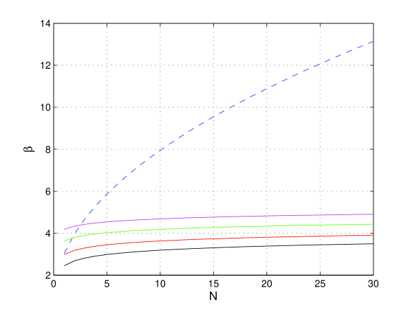
with i=1,,r𝑖1𝑟i=1,\ldots,r, where μisubscript𝜇𝑖\mu_{i} and σisubscript𝜎𝑖\sigma_{i} are the mean and the standard deviation of the scalar random variables ηi(x¯θ,u¯θ)subscript𝜂𝑖subscript¯𝑥𝜃subscript¯𝑢𝜃\eta_{i}(\bar{x}_{\theta},\bar{u}_{\theta}), and smaller values of the constant β𝛽\beta correspond to less conservative approximations of the original chance constraint. For a given value of α𝛼\alpha, the value of β𝛽\beta depends on the number of constraints r𝑟r in a way that differs in the two cases. In the confidence ellipsoid method, in particular, the value of β𝛽\beta is determined by Nn𝑁𝑛Nn (the total dimension of the process noise) when rNn𝑟𝑁𝑛r\geq Nn. In Figure 1, we compare the growth of β𝛽\beta in the two approaches under the assumption that r𝑟r grows linearly with the horizon length N𝑁N. (For the constraint separation method we choose α1==αr=α/rsubscript𝛼1subscript𝛼𝑟𝛼𝑟\alpha_{1}=\ldots=\alpha_{r}=\alpha/r, so that the value of β𝛽\beta is the same for all constraints.)

Refer to caption
Figure 1: Values of β𝛽\beta as a function of the horizon length N𝑁N for the ellipsoidal method (dashed line) and the constraint separation method (solid lines). It is assumed that r=Nr¯(n+m)𝑟𝑁¯𝑟𝑛𝑚r=N\cdot\bar{r}\cdot(n+m), where n=5𝑛5n=5 is the dimension of the system state and of the process noise, m=2𝑚2m=2 is the dimension of the input u𝑢u. r¯¯𝑟\bar{r} reflects the number of constraints per stage; we take r¯=2,10,100,1000¯𝑟2101001000\bar{r}=2,10,100,1000. The value of β𝛽\beta is invariant with respect to r¯¯𝑟\bar{r} (single dashed line) for the ellipsoidal method, while it increases with r¯¯𝑟\bar{r} (multiple solid lines) for the constraint separation method.

The increase of β𝛽\beta is quite rapid in the confidence ellipsoid method, which is only effective for a small number of constraints. An explanation of this phenomenon is provided by the following fact, that is better known by the name of (classical) “concentration of measure” inequalities; proofs may be found in, e.g., [10].

Proposition 8.

Let Γh,ΣsubscriptΓsuperscriptΣ\Gamma_{h,\Sigma^{\prime}} be the r𝑟r-dimensional Gaussian measure with mean hh and (nonsingular) covariance ΣsuperscriptΣ\Sigma^{\prime}, i.e.,

Γh,Σ(dξ)=1(2π)r/2detΣexp(12ξh,Σ1(ξh))dξ.subscriptΓsuperscriptΣd𝜉1superscript2𝜋𝑟2superscriptΣ12𝜉superscriptΣ1𝜉d𝜉\Gamma_{h,\Sigma^{\prime}}(\mathrm{d}\xi)=\frac{1}{(2\pi)^{r/2}\sqrt{\det\Sigma^{\prime}}}\exp\biggl{(}-\frac{1}{2}\left\langle{\xi-h},{\Sigma^{\prime-1}(\xi-h)}\right\rangle\biggr{)}\mathrm{d}\xi.

Then for ε]0,1[\varepsilon\in\;]0,1[,

  1. (i)

    Γh,Σ({ξ|ξhΣ1>r1ε})erε24subscriptΓsuperscriptΣconditional-set𝜉subscriptdelimited-∥∥𝜉superscriptΣ1𝑟1𝜀superscripte𝑟superscript𝜀24\displaystyle{\Gamma_{h,\Sigma^{\prime}}\biggl{(}\biggl{\{}\xi\;\bigg{|}\left\lVert{\xi-h}\right\rVert_{\Sigma^{\prime-1}}>\sqrt{\frac{r}{1-\varepsilon}}\biggr{\}}\biggr{)}\leq\mathrm{e}^{-\frac{r\varepsilon^{2}}{4}}};

  2. (ii)

    Γh,Σ({ξ|ξhΣ1<r(1ε)})erε24subscriptΓsuperscriptΣconditional-set𝜉subscriptdelimited-∥∥𝜉superscriptΣ1𝑟1𝜀superscripte𝑟superscript𝜀24\displaystyle{\Gamma_{h,\Sigma^{\prime}}\bigl{(}\bigl{\{}\xi\big{|}\left\lVert{\xi-h}\right\rVert_{\Sigma^{\prime-1}}<\sqrt{r(1-\varepsilon)}\bigr{\}}\bigr{)}\leq\mathrm{e}^{-\frac{r\varepsilon^{2}}{4}}}.

The above proposition states that as the dimension r𝑟r of the Gaussian measure increases, its mass concentrates in an ellipsoidal shell of ‘mean-size’ r𝑟\sqrt{r}. It readily follows that since η(x¯θ,u¯θ)𝜂subscript¯𝑥𝜃subscript¯𝑢𝜃\eta(\bar{x}_{\theta},\bar{u}_{\theta}) is a r𝑟r-dimensional Gaussian random vector, its mass concentrates around a shell of size r𝑟\sqrt{r}. Note that the bounds corresponding to (i) and (ii) of Proposition 8 in the case of η(x¯θ,u¯θ)𝜂subscript¯𝑥𝜃subscript¯𝑢𝜃\eta(\bar{x}_{\theta},\bar{u}_{\theta}) are independent of the optimization parameters θ𝜃\theta; of course the relative sizes of the confidence ellipsoids change with θ𝜃\theta (because the mean and the covariance of η(x¯θ,u¯θ)𝜂subscript¯𝑥𝜃subscript¯𝑢𝜃\eta(\bar{x}_{\theta},\bar{u}_{\theta}) depend on θ𝜃\theta), but Proposition 8 shows that the size of the confidence ellipsoids grow quite rapidly with the dimension of the noise and the length of the optimization horizon. Intuitively one would expect the ellipsoidal constraint approximation method to be more effective than the cruder approximation by constraint separation. Figure 1 and Proposition 8 however suggest that this is not the case in general; for large numbers of constraints (e.g. longer MPC prediction horizon) the constraint separation method is the less conservative.

3.2.4 Approximation via expectations

For any r𝑟r-dimensional random vector η𝜂\eta, we have 1(η0)=𝔼[1i=1r𝟏],0](ηi)]1-\mathbb{P}\bigl{(}\eta\leq 0\bigr{)}=\mathbb{E}\left[1-\prod_{i=1}^{r}\mathbf{1}_{]-\infty,0]}(\eta_{i})\right]. Using this fact one can arrive at conservative convex approximations of the chance-constraint (18) by replacing the function in the expectation with appropriate approximating functions. For ti>0subscript𝑡𝑖0t_{i}>0, i=1,,r𝑖1𝑟i=1,\ldots,r, consider

φ(η)=i=1rexp(tiηi).𝜑𝜂superscriptsubscript𝑖1𝑟subscript𝑡𝑖subscript𝜂𝑖\varphi(\eta)=\sum_{i=1}^{r}{\exp(t_{i}\eta_{i})}.
Lemma 9.

For any r𝑟r-dimensional random vector η𝜂\eta, 𝔼[φ(η)]1[η0]𝔼delimited-[]𝜑𝜂1delimited-[]𝜂0\mathbb{E}[\varphi(\eta)]\geq 1-\mathbb{P}[\eta\leq 0].

Proof.

For every fixed value of η𝜂\eta, it holds that φ(η)1i=1r𝟏],0](ηi)\varphi(\eta)\geq 1-\prod_{i=1}^{r}\mathbf{1}_{]-\infty,0]}(\eta_{i}). Hence 𝔼[φ(η)]𝔼[1i=1r𝟏],0](ηi)]=1[η0]\mathbb{E}[\varphi(\eta)]\geq\mathbb{E}[1-\prod_{i=1}^{r}\mathbf{1}_{]-\infty,0]}(\eta_{i})]=1-\mathbb{P}[\eta\leq 0]. ∎

Proposition 10.

Under Assumption 2, for η𝜂\eta defined as in (20), it holds that

𝔼[φ(η(x¯θ,u¯θ))]=i=1rexp(tihi,θ+ti22Σ¯12Pi,θ2).𝔼delimited-[]𝜑𝜂subscript¯𝑥𝜃subscript¯𝑢𝜃superscriptsubscript𝑖1𝑟subscript𝑡𝑖subscript𝑖𝜃superscriptsubscript𝑡𝑖22superscriptnormsuperscript¯Σ12subscript𝑃𝑖𝜃2\mathbb{E}\big{[}\varphi\big{(}\eta(\bar{x}_{\theta},\bar{u}_{\theta})\big{)}\big{]}=\sum_{i=1}^{r}\exp\Big{(}t_{i}h_{i,\theta}+\frac{t_{i}^{2}}{2}||\bar{\Sigma}^{\frac{1}{2}}P_{i,\theta}||^{2}\Big{)}.

As a consequence, under Assumption 1 and for any choice of ti>0subscript𝑡𝑖0t_{i}>0, i=1,,r𝑖1𝑟i=1,\ldots,r, the problem

infθΘsubscriptinfimum𝜃Θ\displaystyle\inf_{\theta\in\Theta}\quad 𝔼[V(x¯θ,u¯θ)]𝔼delimited-[]𝑉subscript¯𝑥𝜃subscript¯𝑢𝜃\displaystyle\mathbb{E}[V(\bar{x}_{\theta},\bar{u}_{\theta})]
subjecttosubjectto\displaystyle\mathrm{subject~{}to}\quad (7),(9)andi=1rexp(tihi,θ+ti22Σ¯12Pi,θ2)αitalic-(7italic-)italic-(9italic-)andsuperscriptsubscript𝑖1𝑟subscript𝑡𝑖subscript𝑖𝜃superscriptsubscript𝑡𝑖22superscriptnormsuperscript¯Σ12subscript𝑃𝑖𝜃2𝛼\displaystyle\eqref{e:ubardef},~{}\eqref{eq:cloopsys}~{}\mathrm{and}~{}\sum_{i=1}^{r}\exp\Big{(}t_{i}h_{i,\theta}+\frac{t_{i}^{2}}{2}||\bar{\Sigma}^{\frac{1}{2}}P_{i,\theta}||^{2}\Big{)}\leq\alpha

is a convex conservative approximation of Problem (16)–(18).

Proof.

It is easily seen that, for any r𝑟r-dimensional Gaussian random vector η𝜂\eta with mean μ𝜇\mu and covariance matrix ΣsuperscriptΣ\Sigma^{\prime}, and any vector cr𝑐superscript𝑟c\in\mathbb{R}^{r}, 𝔼[exp(cTη)]=exp(cTμ+12cTΣc)𝔼delimited-[]superscript𝑐𝑇𝜂superscript𝑐𝑇𝜇12superscript𝑐𝑇superscriptΣ𝑐\mathbb{E}\bigl{[}\exp(c^{T}\eta)\bigr{]}=\exp\bigl{(}c^{T}\mu+\frac{1}{2}c^{T}\Sigma^{\prime}c\bigr{)}. Let us now write ηθsubscript𝜂𝜃\eta_{\theta} in place of η(x¯θ,u¯θ)𝜂subscript¯𝑥𝜃subscript¯𝑢𝜃\eta(\bar{x}_{\theta},\bar{u}_{\theta}) for shortness. By the hypotheses on w¯¯𝑤\bar{w}, in the light of (21), ηθsubscript𝜂𝜃\eta_{\theta} is Gaussian with mean hθsubscript𝜃h_{\theta} and covariance PθΣ¯PθTsubscript𝑃𝜃¯Σsuperscriptsubscript𝑃𝜃𝑇P_{\theta}\bar{\Sigma}P_{\theta}^{T}. Then, for a vector cirsubscript𝑐𝑖superscript𝑟c_{i}\in\mathbb{R}^{r} with zero entries except for a coefficient tisubscript𝑡𝑖t_{i} in the i𝑖i-th position,

𝔼[exp(ciTηθ)]=exp(ciThθ+12ciTPθΣ¯PθTci)=exp(tihi,θ+ti22Pi,θTΣ¯Pi,θ).𝔼delimited-[]superscriptsubscript𝑐𝑖𝑇subscript𝜂𝜃superscriptsubscript𝑐𝑖𝑇subscript𝜃12superscriptsubscript𝑐𝑖𝑇subscript𝑃𝜃¯Σsuperscriptsubscript𝑃𝜃𝑇subscript𝑐𝑖subscript𝑡𝑖subscript𝑖𝜃superscriptsubscript𝑡𝑖22superscriptsubscript𝑃𝑖𝜃𝑇¯Σsubscript𝑃𝑖𝜃\mathbb{E}[\exp(c_{i}^{T}\eta_{\theta})]=\exp\Big{(}c_{i}^{T}h_{\theta}+\frac{1}{2}c_{i}^{T}P_{\theta}\bar{\Sigma}P_{\theta}^{T}c_{i}\Big{)}=\exp\Big{(}t_{i}h_{i,\theta}+\frac{t_{i}^{2}}{2}P_{i,\theta}^{T}\bar{\Sigma}P_{i,\theta}\Big{)}.

Summing up for i=1,,r𝑖1𝑟i=1,\ldots,r yields the first result. In order to prove the second statement, note that

𝔼[φ(ηθ)]αiff𝔼delimited-[]𝜑subscript𝜂𝜃𝛼absent\displaystyle\mathbb{E}\bigl{[}\varphi(\eta_{\theta})\bigr{]}\leq\alpha\iff log𝔼[φ(ηθ)]logα𝔼delimited-[]𝜑subscript𝜂𝜃𝛼\displaystyle\log\mathbb{E}\bigl{[}\varphi(\eta_{\theta})\bigr{]}\leq\log\alpha
iff\displaystyle\iff log(i=1rexp(tihi,θ+ti22Σ¯12Pi,θ2))log(α).superscriptsubscript𝑖1𝑟subscript𝑡𝑖subscript𝑖𝜃superscriptsubscript𝑡𝑖22superscriptdelimited-∥∥superscript¯Σ12subscript𝑃𝑖𝜃2𝛼\displaystyle\log\Biggl{(}\sum_{i=1}^{r}{\exp\Bigl{(}t_{i}h_{i,\theta}+\frac{t_{i}^{2}}{2}\left\lVert{\bar{\Sigma}^{\frac{1}{2}}P_{i,\theta}}\right\rVert^{2}\Bigr{)}}\Biggr{)}\leq\log(\alpha).

For each i𝑖i, tihi,θ+ti22Σ¯12Pi,θ2subscript𝑡𝑖subscript𝑖𝜃superscriptsubscript𝑡𝑖22superscriptdelimited-∥∥superscript¯Σ12subscript𝑃𝑖𝜃2t_{i}h_{i,\theta}+\frac{t_{i}^{2}}{2}\left\lVert{\bar{\Sigma}^{\frac{1}{2}}P_{i,\theta}}\right\rVert^{2} is a convex function of the optimization parameters θ𝜃\theta. By [11, Example 3.14], given convex functions g1(θ),,gr(θ)subscript𝑔1𝜃subscript𝑔𝑟𝜃g_{1}(\theta),\ldots,g_{r}(\theta), the function f(θ)=log(eg1(θ)++egk(θ))𝑓𝜃superscript𝑒subscript𝑔1𝜃superscript𝑒subscript𝑔𝑘𝜃f(\theta)=\log\bigl{(}e^{g_{1}(\theta)}+\cdots+e^{g_{k}(\theta)}\bigr{)} is itself convex. It follows that log𝔼[φ(ηθ)]𝔼delimited-[]𝜑subscript𝜂𝜃\log\mathbb{E}\bigl{[}\varphi(\eta_{\theta})\bigr{]} is a convex function of θ𝜃\theta and that the constraint set

{θΘ:log𝔼[φ(ηθ)]logα}={θΘ:𝔼[φ(ηθ)]α}conditional-set𝜃Θ𝔼delimited-[]𝜑subscript𝜂𝜃𝛼conditional-set𝜃Θ𝔼delimited-[]𝜑subscript𝜂𝜃𝛼\{\theta\in\Theta:~{}\log\mathbb{E}[\varphi(\eta_{\theta})]\leq\log\alpha\}=\{\theta\in\Theta:~{}\mathbb{E}[\varphi(\eta_{\theta})]\leq\alpha\}

is convex. Finally, from Lemma 9, if 𝔼[φ(ηθ)]α𝔼delimited-[]𝜑subscript𝜂𝜃𝛼\mathbb{E}[\varphi(\eta_{\theta})]\leq\alpha then [ηθ0]1𝔼[φ(ηθ)]1αdelimited-[]subscript𝜂𝜃01𝔼delimited-[]𝜑subscript𝜂𝜃1𝛼\mathbb{P}[\eta_{\theta}\leq 0]\geq 1-\mathbb{E}[\varphi(\eta_{\theta})]\geq 1-\alpha. Together with Assumption 1, this implies that the optimization problem with constraint i=1rexp(tihi,θ+ti22Σ¯12Pi,θ2)αsuperscriptsubscript𝑖1𝑟subscript𝑡𝑖subscript𝑖𝜃superscriptsubscript𝑡𝑖22superscriptnormsuperscript¯Σ12subscript𝑃𝑖𝜃2𝛼\sum_{i=1}^{r}\exp\Big{(}t_{i}h_{i,\theta}+\frac{t_{i}^{2}}{2}||\bar{\Sigma}^{\frac{1}{2}}P_{i,\theta}||^{2}\Big{)}\leq\alpha in place of (18) is a convex conservative approximation of (16)–(18). ∎

This convex approximation of Problem (16)–(18) is obtained in (13)–(15) by setting R=1𝑅1R=1 and ϕ(η)=φ(η)αitalic-ϕ𝜂𝜑𝜂𝛼\phi(\eta)=\varphi(\eta)-\alpha. The result that the approximation is conservative relies essentially on the fact that, with this choice, ϕ(η)ϕCC(η)italic-ϕ𝜂subscriptitalic-ϕ𝐶𝐶𝜂\phi(\eta)\geq\phi_{CC}(\eta) ηrfor-all𝜂superscript𝑟\forall\eta\in\mathbb{R}^{r} (see Lemma 9). This result can be generalized: Given any two functions ϕ,ϕ′′:r:superscriptitalic-ϕsuperscriptitalic-ϕ′′superscript𝑟\phi^{\prime},\phi^{\prime\prime}:\mathbb{R}^{r}\to\mathbb{R} such that ϕ(η)ϕ′′(η)superscriptitalic-ϕ𝜂superscriptitalic-ϕ′′𝜂\phi^{\prime}(\eta)\geq\phi^{\prime\prime}(\eta) ηrfor-all𝜂superscript𝑟\forall\eta\in\mathbb{R}^{r}, constraint (15) with ϕ=ϕitalic-ϕsuperscriptitalic-ϕ\phi=\phi^{\prime} is more conservative than the same constraint with ϕ=ϕ′′italic-ϕsuperscriptitalic-ϕ′′\phi=\phi^{\prime\prime}. This type of analysis can be exploited to compare different probabilistic constraints and to minimize the conservatism of the convex approximations with respect with the tunable parameters, but is not fully pursued here.

3.3 Ellipsoidal Constraint Functions

Consider the constraint function

η(x¯θ,u¯θ)=([x¯θu¯θ]δ)TΞ([x¯θu¯θ]δ)1,𝜂subscript¯𝑥𝜃subscript¯𝑢𝜃superscriptmatrixsubscript¯𝑥𝜃subscript¯𝑢𝜃𝛿𝑇Ξmatrixsubscript¯𝑥𝜃subscript¯𝑢𝜃𝛿1\eta(\bar{x}_{\theta},\bar{u}_{\theta})=\left(\begin{bmatrix}\bar{x}_{\theta}\\ \bar{u}_{\theta}\end{bmatrix}-\delta\right)^{T}\Xi\left(\begin{bmatrix}\bar{x}_{\theta}\\ \bar{u}_{\theta}\end{bmatrix}-\delta\right)-1,

where Ξ0Ξ0\Xi\geq 0 and δ𝛿\delta are given. Then the constraint η(x¯θ,u¯θ)0𝜂subscript¯𝑥𝜃subscript¯𝑢𝜃0\eta(\bar{x}_{\theta},\bar{u}_{\theta})\leq 0 restricts the vector [x¯θTu¯θT]Tsuperscriptmatrixsuperscriptsubscript¯𝑥𝜃𝑇superscriptsubscript¯𝑢𝜃𝑇𝑇\begin{bmatrix}\bar{x}_{\theta}^{T}&\bar{u}_{\theta}^{T}\end{bmatrix}^{T} to an ellipsoid with center δ𝛿\delta and shape determined by ΞΞ\Xi. We now provide an approximation of the chance constraint (18) that is a semi-definite program in the optimization parameters θ=(G¯,d¯)𝜃¯𝐺¯𝑑\theta=(\bar{G},\bar{d}). Similar to §3.2.2, the idea is to ensure that the 100(1α)%100percent1𝛼100(1-\alpha)\% confidence ellipsoid of w¯¯𝑤\bar{w} is such that (18) holds. To this end, let

yθ=[x¯θu¯θ]δ=[A¯x0+B¯(G¯w¯+d¯)+D¯w¯G¯w¯+d¯]δ=hθ+Pθw¯,subscript𝑦𝜃matrixsubscript¯𝑥𝜃subscript¯𝑢𝜃𝛿matrix¯𝐴subscript𝑥0¯𝐵¯𝐺¯𝑤¯𝑑¯𝐷¯𝑤¯𝐺¯𝑤¯𝑑𝛿superscriptsubscript𝜃superscriptsubscript𝑃𝜃¯𝑤y_{\theta}=\begin{bmatrix}\bar{x}_{\theta}\\ \bar{u}_{\theta}\end{bmatrix}-\delta=\begin{bmatrix}\bar{A}x_{0}+\bar{B}(\bar{G}\bar{w}+\bar{d})+\bar{D}\bar{w}\\ \bar{G}\bar{w}+\bar{d}\end{bmatrix}-\delta=h_{\theta}^{\prime}+P_{\theta}^{\prime}\bar{w},

where hθ=[A¯x0+B¯d¯d¯]δsuperscriptsubscript𝜃matrix¯𝐴subscript𝑥0¯𝐵¯𝑑¯𝑑𝛿h_{\theta}^{\prime}=\begin{bmatrix}\bar{A}x_{0}+\bar{B}\bar{d}\\ \bar{d}\end{bmatrix}-\delta and Pθ=[B¯G¯+D¯G¯]subscriptsuperscript𝑃𝜃matrix¯𝐵¯𝐺¯𝐷¯𝐺P^{\prime}_{\theta}=\begin{bmatrix}\bar{B}\bar{G}+\bar{D}\\ \bar{G}\end{bmatrix}.

Proposition 11.

Define Sθ=β(α)Ξ12PθΣ¯12subscript𝑆𝜃𝛽𝛼superscriptΞ12subscriptsuperscript𝑃𝜃superscript¯Σ12S_{\theta}=\beta(\alpha)\Xi^{\frac{1}{2}}P^{\prime}_{\theta}\bar{\Sigma}^{\frac{1}{2}}, with β(α)𝛽𝛼\beta(\alpha) as in Proposition 7, and ξθ=Ξ12hθsubscript𝜉𝜃superscriptΞ12superscriptsubscript𝜃\xi_{\theta}=\Xi^{\frac{1}{2}}h_{\theta}^{\prime}. Then

[λ+10ξθT0λI(Sθ)TξθSθI]0,λ>0,formulae-sequencematrix𝜆10superscriptsubscript𝜉𝜃𝑇0𝜆𝐼superscriptsubscript𝑆𝜃𝑇subscript𝜉𝜃subscript𝑆𝜃𝐼0𝜆0\begin{bmatrix}-\lambda+1&0&\xi_{\theta}^{T}\\ 0&\lambda I&(S_{\theta})^{T}\\ \xi_{\theta}&S_{\theta}&I\end{bmatrix}\geq 0,\qquad\lambda>0, (26)

is a Linear Matrix Inequality (LMI) in the unknown parameters θ𝜃\theta and λ𝜆\lambda. If (θ,λ)𝜃𝜆(\theta,\lambda) is a solution of (26), then θ𝜃\theta satisfies (18). As a consequence, under Assumption 1, the problem

infθΘ,λsubscriptinfimum𝜃Θ𝜆\displaystyle\inf_{\theta\in\Theta,\lambda}\quad 𝔼[V(x¯θ,u¯θ)]𝔼delimited-[]𝑉subscript¯𝑥𝜃subscript¯𝑢𝜃\displaystyle\mathbb{E}[V(\bar{x}_{\theta},\bar{u}_{\theta})]
subjecttosubjectto\displaystyle\mathrm{subject~{}to}\quad (7),(9)and(26)italic-(7italic-)italic-(9italic-)anditalic-(26italic-)\displaystyle\eqref{e:ubardef},~{}\eqref{eq:cloopsys}~{}\mathrm{and}~{}\eqref{e:bigge}

is a convex conservative approximation of Problem (16)–(18).

Proof.

The inequality (18) may be equivalently represented as

(yθTΞyθ\displaystyle\mathbb{P}\bigl{(}y_{\theta}^{T}\Xi y_{\theta} 10)1α\displaystyle-1\leq 0\bigr{)}\geq 1-\alpha
iff\displaystyle\iff (Ξ12yθ210)1αsuperscriptnormsuperscriptΞ12subscript𝑦𝜃2101𝛼\displaystyle\;\;\mathbb{P}\bigl{(}\|\Xi^{\frac{1}{2}}y_{\theta}\|^{2}-1\leq 0\bigr{)}\geq 1-\alpha
iff\displaystyle\iff (Ξ12(hθ+Pθw¯)210)1αsuperscriptnormsuperscriptΞ12subscriptsuperscript𝜃subscriptsuperscript𝑃𝜃¯𝑤2101𝛼\displaystyle\;\;\mathbb{P}\bigl{(}\|\Xi^{\frac{1}{2}}(h^{\prime}_{\theta}+P^{\prime}_{\theta}\bar{w})\|^{2}-1\leq 0\bigr{)}\geq 1-\alpha
iff\displaystyle\iff (ξθ+Sθw¯210)1α,superscriptnormsubscript𝜉𝜃subscriptsuperscript𝑆𝜃¯𝑤2101𝛼\displaystyle\;\;\mathbb{P}\bigl{(}\|\xi_{\theta}+S^{\prime}_{\theta}\bar{w}\|^{2}-1\leq 0\bigr{)}\geq 1-\alpha, (27)

where Sθ=Ξ12Pθsubscriptsuperscript𝑆𝜃superscriptΞ12subscriptsuperscript𝑃𝜃S^{\prime}_{\theta}=\Xi^{\frac{1}{2}}P^{\prime}_{\theta}. Since w¯𝒩(0,Σ¯)similar-to¯𝑤𝒩0¯Σ\bar{w}\sim\mathcal{N}(0,\bar{\Sigma}), one can compute β(α)>0𝛽𝛼0\beta(\alpha)>0 such that Σ¯1/2w¯2β(α)2superscriptdelimited-∥∥superscript¯Σ12¯𝑤2𝛽superscript𝛼2\left\lVert{\bar{\Sigma}^{-1/2}\bar{w}}\right\rVert^{2}\leq\beta(\alpha)^{2} specifies the required 100(1α)%100percent1𝛼100(1-\alpha)\% confidence ellipsoid of w¯¯𝑤\bar{w}. Hence, we need to ensure that Σ¯1/2w¯2β(α)2ξθ+Sθw¯21superscriptdelimited-∥∥superscript¯Σ12¯𝑤2𝛽superscript𝛼2superscriptdelimited-∥∥subscript𝜉𝜃subscriptsuperscript𝑆𝜃¯𝑤21\left\lVert{\bar{\Sigma}^{-1/2}\bar{w}}\right\rVert^{2}\leq\beta(\alpha)^{2}\Rightarrow\left\lVert{\xi_{\theta}+S^{\prime}_{\theta}\bar{w}}\right\rVert^{2}\leq 1. This is equivalent to

supΣ¯1/2w¯2β(α)2ξθ+Sθw¯21supv¯21ξθ+Sθv¯21.formulae-sequencesubscriptsupremumsuperscriptdelimited-∥∥superscript¯Σ12¯𝑤2𝛽superscript𝛼2superscriptdelimited-∥∥subscript𝜉𝜃subscriptsuperscript𝑆𝜃¯𝑤21iffsubscriptsupremumsuperscriptdelimited-∥∥¯𝑣21superscriptdelimited-∥∥subscript𝜉𝜃subscript𝑆𝜃¯𝑣21\sup_{\left\lVert{\bar{\Sigma}^{-1/2}\bar{w}}\right\rVert^{2}\leq\beta(\alpha)^{2}}\left\lVert{\xi_{\theta}+S^{\prime}_{\theta}\bar{w}}\right\rVert^{2}\leq 1\quad\iff\quad\sup_{\left\lVert{\bar{v}}\right\rVert^{2}\leq 1}\left\lVert{\xi_{\theta}+S_{\theta}\bar{v}}\right\rVert^{2}\leq 1.

It follows from [11, p. 653] that supv¯1ξθ+Sθv¯21subscriptsupremumdelimited-∥∥¯𝑣1superscriptdelimited-∥∥subscript𝜉𝜃subscript𝑆𝜃¯𝑣21\sup_{\left\lVert{\bar{v}}\right\rVert\leq 1}\left\lVert{\xi_{\theta}+S_{\theta}\bar{v}}\right\rVert^{2}\leq 1 if and only if there exists λ0𝜆0\lambda\geq 0 such that

[ξθTξθλ+1ξθTSθ(Sθ)TξθλI(Sθ)TSθ]0.matrixsuperscriptsubscript𝜉𝜃𝑇subscript𝜉𝜃𝜆1superscriptsubscript𝜉𝜃𝑇subscript𝑆𝜃superscriptsubscript𝑆𝜃𝑇subscript𝜉𝜃𝜆𝐼superscriptsubscript𝑆𝜃𝑇subscript𝑆𝜃0\begin{bmatrix}-\xi_{\theta}^{T}\xi_{\theta}-\lambda+1&\xi_{\theta}^{T}S_{\theta}\\ (S_{\theta})^{T}\xi_{\theta}&\lambda I-(S_{\theta})^{T}S_{\theta}\end{bmatrix}\geq 0.

Using Schur complements the last relation can be rewritten equivalently as (26). Therefore, any solution of (26) implies (18). To verify that (26) is an LMI, note that Sθsubscript𝑆𝜃S_{\theta} and ξθsubscript𝜉𝜃\xi_{\theta} are affine in the optimization variables. Together with the assumed convexity of 𝔼[V(x¯θ,u¯θ)]𝔼delimited-[]𝑉subscript¯𝑥𝜃subscript¯𝑢𝜃\mathbb{E}[V(\bar{x}_{\theta},\bar{u}_{\theta})], the last statement of the proposition follows. ∎

4 Integrated chance constraints

In this section we focus on the problem

infθΘsubscriptinfimum𝜃Θ\displaystyle\inf_{\theta\in\Theta}\quad 𝔼[V(x¯θ,u¯θ)]𝔼delimited-[]𝑉subscript¯𝑥𝜃subscript¯𝑢𝜃\displaystyle\mathbb{E}[V(\bar{x}_{\theta},\bar{u}_{\theta})] (28)
subject to (7),(9) anditalic-(7italic-)italic-(9italic-) and\displaystyle\eqref{e:ubardef},~{}\eqref{eq:cloopsys}\textrm{ and} (29)
Ji(θ)βi,i=1,,rformulae-sequencesubscript𝐽𝑖𝜃subscript𝛽𝑖𝑖1𝑟\displaystyle J_{i}(\theta)\leq\beta_{i},~{}i=1,\ldots,r (30)

where, for i=1,,r𝑖1𝑟i=1,\ldots,r, Ji(θ)𝔼[φiηi(x¯θ,u¯θ)]subscript𝐽𝑖𝜃𝔼delimited-[]subscript𝜑𝑖subscript𝜂𝑖subscript¯𝑥𝜃subscript¯𝑢𝜃J_{i}(\theta)\triangleq\mathbb{E}[\varphi_{i}\circ\eta_{i}(\bar{x}_{\theta},\bar{u}_{\theta})], functions φi::subscript𝜑𝑖\varphi_{i}:\mathbb{R}\to\mathbb{R} are measurable and the βi>0subscript𝛽𝑖0\beta_{i}>0 are fixed parameters. This problem corresponds to Problem (13)–(15) when setting R=r𝑅𝑟R=r and ϕi(η)=φi(η)βisubscriptitalic-ϕ𝑖𝜂subscript𝜑𝑖𝜂subscript𝛽𝑖\phi_{i}(\eta)=\varphi_{i}(\eta)-\beta_{i}, with i=1,,r𝑖1𝑟i=1,\ldots,r. For the choice

φi(z)={0,if z0,z,otherwise,subscript𝜑𝑖𝑧cases0if 𝑧0𝑧otherwise\varphi_{i}(z)=\begin{cases}0,&\textrm{if }z\leq 0,\\ z,&\textrm{otherwise},\end{cases} (31)

constraints of the form (30) are known as integrated chance constraints [19, 20]. In fact, one may write (dropping the dependence of ηisubscript𝜂𝑖\eta_{i} on x¯θsubscript¯𝑥𝜃\bar{x}_{\theta} and u¯θsubscript¯𝑢𝜃\bar{u}_{\theta} to simplify the notation)

𝔼[φi(ηi)]=𝔼[0+𝟏[0,ηi)(s)ds]=0+(ηi>s)ds,𝔼delimited-[]subscript𝜑𝑖subscript𝜂𝑖𝔼delimited-[]superscriptsubscript0subscript10subscript𝜂𝑖𝑠differential-d𝑠superscriptsubscript0subscript𝜂𝑖𝑠differential-d𝑠\mathbb{E}[\varphi_{i}(\eta_{i})]=\mathbb{E}\left[\int_{0}^{+\infty}\mathbf{1}_{[0,\eta_{i})}(s)\,\mathrm{d}s\right]=\int_{0}^{+\infty}\mathbb{P}\bigl{(}\eta_{i}>s\bigr{)}\,\mathrm{d}s,

where 𝟏S()subscript1𝑆\mathbf{1}_{S}(\cdot) is the indicator function of set S𝑆S and the second equality follows from Tonelli’s theorem [16, Theorem 4.4.5]. Therefore, constraint (30) is equivalent to

0+(ηi(x¯θ,u¯θ)>s)dsβi,superscriptsubscript0subscript𝜂𝑖subscript¯𝑥𝜃subscript¯𝑢𝜃𝑠differential-d𝑠subscript𝛽𝑖\int_{0}^{+\infty}\mathbb{P}\bigl{(}\eta_{i}(\bar{x}_{\theta},\bar{u}_{\theta})>s\bigr{)}\,\mathrm{d}s\leq\beta_{i}, (32)

whence the name integrated chance constraint. Note that φisubscript𝜑𝑖\varphi_{i} plays the role of a penalty (or barrier) function that penalizes violations of the inequality ηi(x¯,u¯)0subscript𝜂𝑖¯𝑥¯𝑢0\eta_{i}(\bar{x},\bar{u})\leq 0, and βisubscript𝛽𝑖\beta_{i} is a maximum allowable cost in the sense of (32). Of course, different choices of φisubscript𝜑𝑖\varphi_{i} will not guarantee the equivalence between (30) and (32). However, they may be useful in deriving other quantitative chance constraint-type approximations.

4.1 Convexity of Integrated Chance Constraints

We now establish sufficient conditions on the ηisubscript𝜂𝑖\eta_{i} and φisubscript𝜑𝑖\varphi_{i} for the convexity of the constraint set

ICC{θ:Ji(θ)βi,i=1,,r}.subscriptICCconditional-set𝜃formulae-sequencesubscript𝐽𝑖𝜃subscript𝛽𝑖𝑖1𝑟\mathscr{F}_{\rm ICC}\triangleq\{\theta:~{}J_{i}(\theta)\leq\beta_{i},~{}i=1,\ldots,r\}. (33)

The result is again a consequence of Proposition 3.

Proposition 12.

Let the mappings ηi:(N+1)n×Nm:subscript𝜂𝑖superscript𝑁1𝑛𝑁𝑚\eta_{i}:\mathbb{R}^{(N+1)n\times Nm}\to\mathbb{R} be measurable and convex, and let the φi::subscript𝜑𝑖\varphi_{i}:\mathbb{R}\to\mathbb{R} be measurable, monotone nondecreasing and convex. Assume that the Ji(θ)subscript𝐽𝑖𝜃J_{i}(\theta) are finite for all θ𝜃\theta. Then each Ji(θ)subscript𝐽𝑖𝜃J_{i}(\theta) is a convex function of θ𝜃\theta and ICCsubscriptICC\mathscr{F}_{\rm ICC} is a convex set. As a consequence, under Assumption 1, (28)–(30) is a convex optimization problem.

Proof.

Fix ωΩ𝜔Ω\omega\in\Omega arbitrarily. Since the mapping θ(x¯θ(ω),u¯θ(ω))maps-to𝜃subscript¯𝑥𝜃𝜔subscript¯𝑢𝜃𝜔\theta\mapsto\big{(}\bar{x}_{\theta}(\omega),\bar{u}_{\theta}(\omega)\big{)} is affine and (x¯,u¯)ηi(x¯,u¯)maps-to¯𝑥¯𝑢subscript𝜂𝑖¯𝑥¯𝑢(\bar{x},\bar{u})\mapsto\eta_{i}(\bar{x},\bar{u}) is convex by assumption, their composition θηi(x¯(ω),u¯(ω))maps-to𝜃subscript𝜂𝑖¯𝑥𝜔¯𝑢𝜔\theta\mapsto\eta_{i}\big{(}\bar{x}(\omega),\bar{u}(\omega)\big{)} is a convex function of θ𝜃\theta. Using the assumption that φisubscript𝜑𝑖\varphi_{i} is monotone nondecreasing and convex, we may apply Proposition 3 with γ(ω,θ)=ηi(x¯θ(ω),u¯θ(ω))𝛾𝜔𝜃subscript𝜂𝑖subscript¯𝑥𝜃𝜔subscript¯𝑢𝜃𝜔\gamma(\omega,\theta)=\eta_{i}\big{(}\bar{x}_{\theta}(\omega),\bar{u}_{\theta}(\omega)\big{)} and φisubscript𝜑𝑖\varphi_{i} in place of φ𝜑\varphi to conclude that Ji(θ)=𝔼[φiγ(ω,θ)]subscript𝐽𝑖𝜃𝔼delimited-[]subscript𝜑𝑖𝛾𝜔𝜃J_{i}(\theta)=\mathbb{E}[\varphi_{i}\circ\gamma(\omega,\theta)] is convex. Hence, for any choice of βisubscript𝛽𝑖\beta_{i}, the set i{θ:Ji(θ)βi}subscript𝑖conditional-set𝜃subscript𝐽𝑖𝜃subscript𝛽𝑖\mathscr{F}_{i}\triangleq\{\theta:~{}J_{i}(\theta)\leq\beta_{i}\} is convex. Since ICC=i=1risubscriptICCsuperscriptsubscript𝑖1𝑟subscript𝑖\mathscr{F}_{\rm ICC}=\bigcap_{i=1}^{r}\mathscr{F}_{i}, the convexity of ICCsubscriptICC\mathscr{F}_{\rm ICC} follows. Together with Assumption 1, this proves that (28)–(30) is a convex optimization problem. ∎

It is worth noting that the function φ()𝜑\varphi(\cdot) of Section 3.2.4 satisfies analogous monotonicity and convexity assumptions with respect to each of the ηisubscript𝜂𝑖\eta_{i}, with i=1,,r𝑖1𝑟i=1,\ldots,r. Unlike those of Section 3, this convexity result is independent of the probability distribution of w¯¯𝑤\bar{w}. By virtue of the alternative assumptions (iii) and (iii′′) of Proposition 3, the requirement that J(θ)𝐽𝜃J(\theta) be finite for all θ𝜃\theta may be relaxed. A sufficient requirement is that there exist no two values θ𝜃\theta and θsuperscript𝜃\theta^{\prime} such that J(θ)=+𝐽𝜃J(\theta)=+\infty and J(θ)=𝐽superscript𝜃J(\theta^{\prime})=-\infty. In particular, provided measurable and convex ηisubscript𝜂𝑖\eta_{i}, definition (31) satisfies all the requirements of Proposition 12.

Example 13.

The (scalar) polytopic constraint function:

η(x¯θ,u¯θ)=Txx¯θ+Tuu¯θy𝜂subscript¯𝑥𝜃subscript¯𝑢𝜃subscript𝑇𝑥subscript¯𝑥𝜃subscript𝑇𝑢subscript¯𝑢𝜃𝑦\eta(\bar{x}_{\theta},\bar{u}_{\theta})=T_{x}\bar{x}_{\theta}+T_{u}\bar{u}_{\theta}-y

fulfills the hypotheses of Proposition 12. Hence, the corresponding integrated chance constraint is convex.

Example 14.

Following Example 1, an interesting case is that of ellipsoidal constraints. For an ((N+1)n+Nm)𝑁1𝑛𝑁𝑚\big{(}(N+1)n+Nm\big{)}-size positive-semidefinite real matrix ΞΞ\Xi and a vector δ(N+1)n+Nm𝛿superscript𝑁1𝑛𝑁𝑚\delta\in\mathbb{R}^{(N+1)n+Nm}, define

η(x¯θ,u¯θ)([x¯θu¯θ]δ)TΞ([x¯θu¯θ]δ)1.𝜂subscript¯𝑥𝜃subscript¯𝑢𝜃superscriptmatrixsubscript¯𝑥𝜃subscript¯𝑢𝜃𝛿𝑇Ξmatrixsubscript¯𝑥𝜃subscript¯𝑢𝜃𝛿1\eta(\bar{x}_{\theta},\bar{u}_{\theta})\triangleq\left(\begin{bmatrix}\bar{x}_{\theta}\\ \bar{u}_{\theta}\end{bmatrix}-\delta\right)^{T}\Xi\left(\begin{bmatrix}\bar{x}_{\theta}\\ \bar{u}_{\theta}\end{bmatrix}-\delta\right)-1. (34)

This is a convex function of the vector [x¯θTu¯θT]Tsuperscriptmatrixsuperscriptsubscript¯𝑥𝜃𝑇superscriptsubscript¯𝑢𝜃𝑇𝑇\begin{bmatrix}\bar{x}_{\theta}^{T}&\bar{u}_{\theta}^{T}\end{bmatrix}^{T} (it is the composition of the convex mapping ξTΞξsuperscript𝜉𝑇Ξ𝜉\xi^{T}\Xi\xi, Ξ0Ξ0\Xi\geq 0, with the affine mapping ξ=[x¯θTu¯θT]Tδ𝜉superscriptmatrixsuperscriptsubscript¯𝑥𝜃𝑇superscriptsubscript¯𝑢𝜃𝑇𝑇𝛿\xi=\begin{bmatrix}\bar{x}_{\theta}^{T}&\bar{u}_{\theta}^{T}\end{bmatrix}^{T}-\delta) and hence Proposition 12 applies.

Remark 15.

A problem setting similar to Example 14 with quadratic expected-type cost function and ellipsoidal constraints has been adopted in [26], where hard constraints are relaxed to expected-type constraints of the form 𝔼[η(x¯,u¯)]β𝔼delimited-[]𝜂¯𝑥¯𝑢𝛽\mathbb{E}[\eta(\bar{x},\bar{u})]\leq\beta. This formulation can be seen as a special case of integrated chance constraints with φ(z)=z𝜑𝑧𝑧\varphi(z)=z for all z𝑧z. The choice of φ𝜑\varphi within a large class of functions is an extra degree of freedom provided by our framework that may be exploited to establish tight bounds on the probability of violating the original hard constraints, see Lemma 9 for an example.

4.2 Numerical solution of optimization problems with ICC

Even though ICC problems are convex in general, deriving efficient algorithms to solve them is still a major challenge [19, 20]. For certain ICCs, it is possible however to derive explicit expressions for the gradients of the constraint function. Provided the cost has a simple (e.g. quadratic) form, this allows one to implement standard algorithms (e.g. interior point methods [11]) for the solution of the optimization problem.

Let w¯¯𝑤\bar{w} satisfy Assumption 2 with, for simplicity, Σ¯¯Σ\bar{\Sigma} equal to the identity matrix, i.e. w¯𝒩(0,I)similar-to¯𝑤𝒩0𝐼\bar{w}\sim\mathcal{N}(0,I). Consider the problem with one scalar constraint (the generalization to multiple (joint) constraints is straightforward):

minθsubscript𝜃\displaystyle\min_{\theta} [x¯θTu¯θT]M[x¯θu¯θ]matrixsuperscriptsubscript¯𝑥𝜃𝑇superscriptsubscript¯𝑢𝜃𝑇𝑀matrixsubscript¯𝑥𝜃subscript¯𝑢𝜃\displaystyle\begin{bmatrix}\bar{x}_{\theta}^{T}&\bar{u}_{\theta}^{T}\end{bmatrix}M\begin{bmatrix}\bar{x}_{\theta}\\ \bar{u}_{\theta}\end{bmatrix} (35)
subject to (7),(9) and 𝔼[φ(Txx¯θ+Tuu¯θy)]β,italic-(7italic-)italic-(9italic-) and 𝔼delimited-[]𝜑subscript𝑇𝑥subscript¯𝑥𝜃subscript𝑇𝑢subscript¯𝑢𝜃𝑦𝛽\displaystyle\eqref{e:ubardef},~{}\eqref{eq:cloopsys}\textrm{ and }\mathbb{E}[\varphi(T_{x}\bar{x}_{\theta}+T_{u}\bar{u}_{\theta}-y)]\leq\beta,

where φ𝜑\varphi is defined as in (31).

Lemma 16.

Let z𝑧z be a Gaussian random variable with mean μ𝜇\mu and variance σ2>0superscript𝜎20\sigma^{2}>0. Then

𝔼[φ(z)]=σg(μσ)𝔼delimited-[]𝜑𝑧𝜎𝑔𝜇𝜎\mathbb{E}[\varphi(z)]=\sigma g\Bigl{(}\frac{\mu}{\sigma}\Bigr{)}

where

g(x)=x2erfc(x2)+12πexp(x22)𝑔𝑥𝑥2erfc𝑥212𝜋superscript𝑥22g(x)=\frac{x}{2}\operatorname{erfc}\Bigl{(}\frac{-x}{\sqrt{2}}\Bigr{)}+\frac{1}{\sqrt{2\pi}}\exp\Bigl{(}\frac{-x^{2}}{2}\Bigr{)}

and erfc(x)=1erf(x)erfc𝑥1erf𝑥\operatorname{erfc}(x)=1-\operatorname{erf}(x) is the standard complementary error function.

Proof.

Since z𝒩(μ,σ2)similar-to𝑧𝒩𝜇superscript𝜎2z\sim\mathcal{N}(\mu,\sigma^{2}) it holds that

𝔼[φ(z)]=12πσ20texp((tμ)22σ2)𝑑t.𝔼delimited-[]𝜑𝑧12𝜋superscript𝜎2superscriptsubscript0𝑡superscript𝑡𝜇22superscript𝜎2differential-d𝑡\mathbb{E}[\varphi(z)]=\frac{1}{\sqrt{2\pi\sigma^{2}}}\int_{0}^{\infty}t\exp\left(-\frac{(t-\mu)^{2}}{2\sigma^{2}}\right)\;dt.

By the change of variable y=tμ2σ𝑦𝑡𝜇2𝜎y=\frac{t-\mu}{\sqrt{2}\sigma} one gets

𝔼[φ(z)]=𝔼delimited-[]𝜑𝑧absent\displaystyle\mathbb{E}[\varphi(z)]= 1πμ2σ(μ+2σy)exp(y2)𝑑y1𝜋superscriptsubscript𝜇2𝜎𝜇2𝜎𝑦superscript𝑦2differential-d𝑦\displaystyle\,\,\frac{1}{\sqrt{\pi}}\int_{\frac{-\mu}{\sqrt{2}\sigma}}^{\infty}(\mu+\sqrt{2}\sigma y)\exp(-y^{2})dy
=\displaystyle= μπμ2σexp(y2)𝑑y+σ2πμ2σyexp(y2)𝑑y𝜇𝜋superscriptsubscript𝜇2𝜎superscript𝑦2differential-d𝑦𝜎2𝜋superscriptsubscript𝜇2𝜎𝑦superscript𝑦2differential-d𝑦\displaystyle\,\,\frac{\mu}{\sqrt{\pi}}\int_{\frac{-\mu}{\sqrt{2}\sigma}}^{\infty}\exp(-y^{2})dy+\sigma\sqrt{\frac{2}{\pi}}\int_{\frac{-\mu}{\sqrt{2}\sigma}}^{\infty}y\exp(-y^{2})dy
=\displaystyle= μ2erfc(μ2σ)+σ2πexp(μ22σ2),𝜇2erfc𝜇2𝜎𝜎2𝜋superscript𝜇22superscript𝜎2\displaystyle\,\,\frac{\mu}{2}\operatorname{erfc}\left(\frac{-\mu}{\sqrt{2}\sigma}\right)+\frac{\sigma}{\sqrt{2\pi}}\exp\left(-\frac{\mu^{2}}{2\sigma^{2}}\right),

which is equal to σg(μσ)𝜎𝑔𝜇𝜎\sigma g(\frac{\mu}{\sigma}). ∎

Simple calculations and the application of this lemma yield the following result.

Proposition 17.

Problem (35) is equivalent to

minimize h1(d¯)+h2(G¯)subscript1¯𝑑subscript2¯𝐺\displaystyle h_{1}(\bar{d})+h_{2}(\bar{G}) (36)
subject to σg(μσ)β𝜎𝑔𝜇𝜎𝛽\displaystyle\sigma g\Bigl{(}\frac{\mu}{\sigma}\Bigr{)}\leq\beta

where

μ=𝜇absent\displaystyle\mu= (TxA¯x0y¯)+(TxB¯+Tu)d¯,superscript𝑇𝑥¯𝐴subscript𝑥0¯𝑦superscript𝑇𝑥¯𝐵superscript𝑇𝑢¯𝑑\displaystyle(T^{x}\bar{A}x_{0}-\bar{y})+(T^{x}\bar{B}+T^{u})\bar{d},
σ=𝜎absent\displaystyle\sigma= (TxD¯+(TxB¯+Tu)G¯)T2,subscriptnormsuperscriptsuperscript𝑇𝑥¯𝐷superscript𝑇𝑥¯𝐵superscript𝑇𝑢¯𝐺𝑇2\displaystyle||(T^{x}\bar{D}+(T^{x}\bar{B}+T^{u})\bar{G})^{T}||_{2},
h1(d¯)=subscript1¯𝑑absent\displaystyle h_{1}(\bar{d})= [(A¯x0+B¯d¯)Td¯T]M[A¯x0+B¯d¯d¯],matrixsuperscript¯𝐴subscript𝑥0¯𝐵¯𝑑𝑇superscript¯𝑑𝑇𝑀matrix¯𝐴subscript𝑥0¯𝐵¯𝑑¯𝑑\displaystyle\begin{bmatrix}(\bar{A}x_{0}+\bar{B}\bar{d})^{T}&\bar{d}^{T}\end{bmatrix}M\begin{bmatrix}\bar{A}x_{0}+\bar{B}\bar{d}\\ \bar{d}\end{bmatrix},
h2(G¯)=subscript2¯𝐺absent\displaystyle h_{2}(\bar{G})= Tr([(B¯G¯+D¯)TG¯T]M[B¯G¯+D¯G¯]).Trmatrixsuperscript¯𝐵¯𝐺¯𝐷𝑇superscript¯𝐺𝑇𝑀matrix¯𝐵¯𝐺¯𝐷¯𝐺\displaystyle\text{Tr}\Biggl{(}\begin{bmatrix}(\bar{B}\bar{G}+\bar{D})^{T}&\bar{G}^{T}\end{bmatrix}M\begin{bmatrix}\bar{B}\bar{G}+\bar{D}\\ \bar{G}\end{bmatrix}\Biggr{)}.

Note that expectations have been integrated out. Now it is possible to put the problem in a standard form for numerical optimization. Let G¯isubscript¯𝐺𝑖\bar{G}_{i} and D¯isubscript¯𝐷𝑖\bar{D}_{i} be the i𝑖i-th column of G¯¯𝐺\bar{G} and D¯¯𝐷\bar{D}, respectively. Redefine the optimization variable θ𝜃\theta as the vector θ¯=[d¯TG¯1TG¯NnT]T¯𝜃superscriptmatrixsuperscript¯𝑑𝑇superscriptsubscript¯𝐺1𝑇superscriptsubscript¯𝐺𝑁𝑛𝑇𝑇\bar{\theta}=\begin{bmatrix}\bar{d}^{T}&\bar{G}_{1}^{T}&\cdots&\bar{G}_{Nn}^{T}\end{bmatrix}^{T}. Define e𝑒e, f𝑓f, v𝑣v and L𝐿L by

μ=(TxA¯x0y¯)+(TxB¯+Tu)d¯=𝜇superscript𝑇𝑥¯𝐴subscript𝑥0¯𝑦superscript𝑇𝑥¯𝐵superscript𝑇𝑢¯𝑑absent\displaystyle\mu=(T^{x}\bar{A}x_{0}-\bar{y})+(T^{x}\bar{B}+T^{u})\bar{d}= e+fTθ¯,𝑒superscript𝑓𝑇¯𝜃\displaystyle e+f^{T}\bar{\theta},
(TxD¯+(TxB¯+Tu)G¯)T=superscriptsuperscript𝑇𝑥¯𝐷superscript𝑇𝑥¯𝐵superscript𝑇𝑢¯𝐺𝑇absent\displaystyle(T^{x}\bar{D}+(T^{x}\bar{B}+T^{u})\bar{G})^{T}= v+Lθ¯.𝑣𝐿¯𝜃\displaystyle v+L\bar{\theta}.
Corollary 18.

Problem (35) is equivalent to

minimize f0(θ¯)=minimize subscript𝑓0¯𝜃absent\displaystyle\text{minimize }\quad f_{0}(\bar{\theta})= g0(θ¯)+i=1Nngi(θ¯)subscript𝑔0¯𝜃superscriptsubscript𝑖1𝑁𝑛subscript𝑔𝑖¯𝜃\displaystyle g_{0}(\bar{\theta})+\sum_{i=1}^{Nn}g_{i}(\bar{\theta})
subject to Hθ¯=subject to 𝐻¯𝜃absent\displaystyle\text{subject to }\quad H\bar{\theta}= 0,0\displaystyle 0,
f1(θ¯)subscript𝑓1¯𝜃absent\displaystyle f_{1}(\bar{\theta})\leq 00\displaystyle 0

where the matrix H𝐻H in the equality constraint accounts for the causal structure of G¯¯𝐺\bar{G}, while

g0(θ¯)=subscript𝑔0¯𝜃absent\displaystyle g_{0}(\bar{\theta})= ([A¯x00]+[B¯I]H0θ¯)TM([A¯x00]+[B¯I]H0θ¯),superscriptmatrix¯𝐴subscript𝑥00matrix¯𝐵𝐼subscript𝐻0¯𝜃𝑇𝑀matrix¯𝐴subscript𝑥00matrix¯𝐵𝐼subscript𝐻0¯𝜃\displaystyle\Bigl{(}\begin{bmatrix}\bar{A}x_{0}\\ 0\end{bmatrix}+\begin{bmatrix}\bar{B}\\ I\end{bmatrix}H_{0}\bar{\theta}\Bigr{)}^{T}M\Bigl{(}\begin{bmatrix}\bar{A}x_{0}\\ 0\end{bmatrix}+\begin{bmatrix}\bar{B}\\ I\end{bmatrix}H_{0}\bar{\theta}\Bigr{)},
gi(θ¯)=subscript𝑔𝑖¯𝜃absent\displaystyle g_{i}(\bar{\theta})= ([D¯i0]+[B¯I]Hiθ¯)TM([D¯i0]+[B¯I]Hiθ¯),superscriptmatrixsubscript¯𝐷𝑖0matrix¯𝐵𝐼subscript𝐻𝑖¯𝜃𝑇𝑀matrixsubscript¯𝐷𝑖0matrix¯𝐵𝐼subscript𝐻𝑖¯𝜃\displaystyle\Bigl{(}\begin{bmatrix}\bar{D}_{i}\\ 0\end{bmatrix}+\begin{bmatrix}\bar{B}\\ I\end{bmatrix}H_{i}\bar{\theta}\Bigr{)}^{T}M\Bigl{(}\begin{bmatrix}\bar{D}_{i}\\ 0\end{bmatrix}+\begin{bmatrix}\bar{B}\\ I\end{bmatrix}H_{i}\bar{\theta}\Bigr{)},
f1(θ¯)=subscript𝑓1¯𝜃absent\displaystyle f_{1}(\bar{\theta})= v+Lθ¯g(e+fTθ¯v+Lθ¯)β0,delimited-∥∥𝑣𝐿¯𝜃𝑔𝑒superscript𝑓𝑇¯𝜃delimited-∥∥𝑣𝐿¯𝜃𝛽0\displaystyle\left\lVert{v+L\bar{\theta}}\right\rVert g\Bigl{(}\frac{e+f^{T}\bar{\theta}}{\left\lVert{v+L\bar{\theta}}\right\rVert}\Bigr{)}-\beta\leq 0,

and H0subscript𝐻0H_{0} and Hisubscript𝐻𝑖H_{i} are selection matrices such that H0θ¯=d¯subscript𝐻0¯𝜃¯𝑑H_{0}\bar{\theta}=\bar{d} and Hiθ¯=G¯isubscript𝐻𝑖¯𝜃subscript¯𝐺𝑖H_{i}\bar{\theta}=\bar{G}_{i}.

We conclude the section by documenting the expressions of the gradient and the Hessian of the constraint function f1(θ¯)subscript𝑓1¯𝜃f_{1}(\bar{\theta}).

f1(θ¯)=12πLTv+Lθ¯v+Lθ¯exp((e+fTθ¯)22v+Lθ¯2)+12erfc(e+fTθ¯2v+Lθ¯)fsubscript𝑓1¯𝜃12𝜋superscript𝐿𝑇𝑣𝐿¯𝜃delimited-∥∥𝑣𝐿¯𝜃superscript𝑒superscript𝑓𝑇¯𝜃22superscriptdelimited-∥∥𝑣𝐿¯𝜃212erfc𝑒superscript𝑓𝑇¯𝜃2delimited-∥∥𝑣𝐿¯𝜃𝑓\nabla f_{1}(\bar{\theta})=\frac{1}{\sqrt{2\pi}}L^{T}\frac{v+L\bar{\theta}}{\left\lVert{v+L\bar{\theta}}\right\rVert}\exp{\Bigl{(}-\frac{(e+f^{T}\bar{\theta})^{2}}{2\left\lVert{v+L\bar{\theta}}\right\rVert^{2}}\Bigr{)}}+\frac{1}{2}\operatorname{erfc}{\Bigl{(}-\frac{e+f^{T}\bar{\theta}}{\sqrt{2}\left\lVert{v+L\bar{\theta}}\right\rVert}\Bigr{)}}f

2f1(θ¯)=12πexp((e+fTθ¯)22v+Lθ¯2)[J1(θ¯)+J2(θ¯)J3(θ¯)]superscript2subscript𝑓1¯𝜃12𝜋superscript𝑒superscript𝑓𝑇¯𝜃22superscriptdelimited-∥∥𝑣𝐿¯𝜃2delimited-[]subscript𝐽1¯𝜃subscript𝐽2¯𝜃subscript𝐽3¯𝜃\nabla^{2}f_{1}(\bar{\theta})=\frac{1}{\sqrt{2\pi}}\exp{\Bigl{(}-\frac{(e+f^{T}\bar{\theta})^{2}}{2\left\lVert{v+L\bar{\theta}}\right\rVert^{2}}\Bigr{)}}\Bigl{[}J_{1}(\bar{\theta})+J_{2}(\bar{\theta})-J_{3}(\bar{\theta})\Bigr{]}

where

J1(θ¯)subscript𝐽1¯𝜃\displaystyle J_{1}(\bar{\theta}) =1v+Lθ¯(LTL+ffT),absent1delimited-∥∥𝑣𝐿¯𝜃superscript𝐿𝑇𝐿𝑓superscript𝑓𝑇\displaystyle=\frac{1}{\left\lVert{v+L\bar{\theta}}\right\rVert}(L^{T}L+ff^{T}),
J2(θ¯)subscript𝐽2¯𝜃\displaystyle J_{2}(\bar{\theta}) =((e+fTθ¯)2v+Lθ¯2v+Lθ¯5)(LT(v+Lθ¯)(v+Lθ¯)TL),absentsuperscript𝑒superscript𝑓𝑇¯𝜃2superscriptdelimited-∥∥𝑣𝐿¯𝜃2superscriptdelimited-∥∥𝑣𝐿¯𝜃5superscript𝐿𝑇𝑣𝐿¯𝜃superscript𝑣𝐿¯𝜃𝑇𝐿\displaystyle=\Bigl{(}\frac{(e+f^{T}\bar{\theta})^{2}-\left\lVert{v+L\bar{\theta}}\right\rVert^{2}}{\left\lVert{v+L\bar{\theta}}\right\rVert^{5}}\Bigr{)}(L^{T}(v+L\bar{\theta})(v+L\bar{\theta})^{T}L),
J3(θ¯)subscript𝐽3¯𝜃\displaystyle J_{3}(\bar{\theta}) =(e+fTθ¯v+Lθ¯3)(LT(v+Lθ¯)fT+f(v+Lθ¯)TL).\displaystyle=\Bigl{(}\frac{e+f^{T}\bar{\theta}}{\left\lVert{v+L\bar{\theta}}\right\rVert^{3}}\Bigl{)}(L^{T}(v+L\bar{\theta})f^{T}+f(v+L\bar{\theta})^{T}L).

The expressions of gradient and Hessian of the quadratic function f0(θ¯)subscript𝑓0¯𝜃f_{0}(\bar{\theta}), used e.g. by interior point method solvers, are quite standard and will not be reported here.

5 Simulation results

We illustrate some of our results with the help of a simple example. Consider the mechanical system shown in Figure 2.

\psfrag{d1}[b]{$d_{1}$}\psfrag{d2}[b]{$d_{2}$}\psfrag{d3}[b]{$d_{3}$}\psfrag{d4}[b]{$d_{4}$}\psfrag{m1}{$m_{1}$}\psfrag{m2}{$m_{2}$}\psfrag{m3}{$m_{3}$}\psfrag{m4}{$m_{4}$}\psfrag{k1}[t]{$k_{1}$}\psfrag{k2}[t]{$k_{2}$}\psfrag{k3}[t]{$k_{3}$}\psfrag{k4}[t]{$k_{4}$}\psfrag{u1}[b]{$u_{1}$}\psfrag{u2}[b]{$u_{2}$}\psfrag{u3}[t]{$u_{3}$}\includegraphics[width=390.25534pt]{mass-spring}
Figure 2: A mechanical system with springs and masses.

d1,,d4subscript𝑑1subscript𝑑4d_{1},\cdots,d_{4} are displacements from an equilibrium position, u1,,u3subscript𝑢1subscript𝑢3u_{1},\cdots,u_{3} are forces acting on the masses. In particular, u1subscript𝑢1u_{1} is a tension between the first and the second mass, u2subscript𝑢2u_{2} is a tension between the third and the fourth mass, and u3subscript𝑢3u_{3} is a force between the wall (at left) and the second mass. We assume all mass and stiffness constants to be equal to unity, i.e. m1==m4=1,k1==k4=1formulae-sequencesubscript𝑚1subscript𝑚41subscript𝑘1subscript𝑘41m_{1}=\cdots=m_{4}=1,k_{1}=\cdots=k_{4}=1. We consider a discrete-time model of this system with noise in the dynamics,

x(t+1)=Ax(t)+Bu(t)+w(t),𝑥𝑡1𝐴𝑥𝑡𝐵𝑢𝑡𝑤𝑡x(t+1)=Ax(t)+Bu(t)+w(t),

where w𝑤w is an i.i.d. noise process, w(t)𝒩(0,σ2I),σ=0.05formulae-sequencesimilar-to𝑤𝑡𝒩0superscript𝜎2𝐼𝜎0.05w(t)\sim\mathcal{N}(0,\sigma^{2}I),\sigma=0.05 for all t𝑡t, and x=[d1,d2,d3,d4,d˙1,d˙2,d˙3,d˙4]T𝑥superscriptmatrixsubscript𝑑1subscript𝑑2subscript𝑑3subscript𝑑4subscript˙𝑑1subscript˙𝑑2subscript˙𝑑3subscript˙𝑑4𝑇x=\begin{bmatrix}d_{1},d_{2},d_{3},d_{4},\dot{d}_{1},\dot{d}_{2},\dot{d}_{3},\dot{d}_{4}\end{bmatrix}^{T}. The discrete-time dynamics are obtained by uniform sampling of a continuous-time model at times th𝑡t\cdot h, with sampling time h=11h=1 and t=0,1,2,𝑡012t=0,1,2,\ldots, under the assumption that the control action u(t)𝑢𝑡u(t) is piecewise constant over the sampling intervals [th,th+h)𝑡𝑡[t\cdot h,t\cdot h+h). Hence, A=ehAc𝐴superscript𝑒subscript𝐴𝑐A=e^{hA_{c}} and B=Ac1(ehAcI)Bc𝐵superscriptsubscript𝐴𝑐1superscript𝑒subscript𝐴𝑐𝐼subscript𝐵𝑐B=A_{c}^{-1}(e^{hA_{c}}-I)B_{c}, where Acsubscript𝐴𝑐A_{c} and Bcsubscript𝐵𝑐B_{c}, defined as

Ac=subscript𝐴𝑐absent\displaystyle A_{c}= [04×4I4×4Ac,2104×4],matrixsubscript044subscript𝐼44subscript𝐴𝑐21subscript044\displaystyle\,\,\begin{bmatrix}0_{4\times 4}&I_{4\times 4}\\ A_{c,21}&0_{4\times 4}\end{bmatrix}, Ac,21=subscript𝐴𝑐21absent\displaystyle A_{c,21}= [2100,121001210011],matrix2100121001210011\displaystyle\,\,\begin{bmatrix}-2&1&0&0,\\ 1&-2&1&0\\ 0&1&-2&1\\ 0&0&1&-1\\ \end{bmatrix},
Bc=subscript𝐵𝑐absent\displaystyle B_{c}= [04×3Bc,21],matrixsubscript043subscript𝐵𝑐21\displaystyle\,\,\begin{bmatrix}0_{4\times 3}\\ B_{c,21}\end{bmatrix}, Bc,21=subscript𝐵𝑐21absent\displaystyle B_{c,21}= [100101010010]matrix100101010010\displaystyle\,\,\begin{bmatrix}1&0&0\\ -1&0&-1\\ 0&1&0\\ 0&-1&0\\ \end{bmatrix}

are the state and input matrices of the standard ODE model of the system.

We are interested in computing the control policy that minimizes the cost function

𝔼[t=0N1(x(t)TQx(t)+u(t)TRu(t))+x(N)TQx(N)],𝔼delimited-[]superscriptsubscript𝑡0𝑁1𝑥superscript𝑡𝑇𝑄𝑥𝑡𝑢superscript𝑡𝑇𝑅𝑢𝑡𝑥superscript𝑁𝑇𝑄𝑥𝑁\mathbb{E}\left[\sum_{t=0}^{N-1}\bigl{(}x(t)^{T}Qx(t)+u(t)^{T}Ru(t)\bigr{)}+x(N)^{T}Qx(N)\right],

where the horizon length is fixed to N=5𝑁5N=5, the weight matrices are defined as Q=[I000]𝑄matrix𝐼000Q=\begin{bmatrix}I&0\\ 0&0\end{bmatrix} (penalizing displacements but not their derivatives) and R=I𝑅𝐼R=I. The initial state is set to x0=[0,0,0,1,0,0,0,0]Tsubscript𝑥0superscript00010000𝑇x_{0}=[0,0,0,1,0,0,0,0]^{T}. In the absence of constraints, this is a finite horizon LQG problem whose optimal solution is the linear time-varying feedback from the state

u(t)=(BTP(t+1)B+R)1BTP(t+1)Ax(t),𝑢𝑡superscriptsuperscript𝐵𝑇𝑃𝑡1𝐵𝑅1superscript𝐵𝑇𝑃𝑡1𝐴𝑥𝑡u(t)=-\big{(}B^{T}P(t+1)B+R\big{)}^{-1}B^{T}P(t+1)Ax(t),

where the matrices P(t)𝑃𝑡P(t) are computed by solving, for t=N1,,0𝑡𝑁10t=N-1,\ldots,0, the backward dynamic programming recursion

P(t)=Q+ATP(t+1)AATP(t+1)B(BTP(t+1)B+R)1BTP(t+1)A,𝑃𝑡𝑄superscript𝐴𝑇𝑃𝑡1𝐴superscript𝐴𝑇𝑃𝑡1𝐵superscriptsuperscript𝐵𝑇𝑃𝑡1𝐵𝑅1superscript𝐵𝑇𝑃𝑡1𝐴P(t)=Q+A^{T}P(t+1)A-A^{T}P(t+1)B(B^{T}P(t+1)B+R)^{-1}B^{T}P(t+1)A,

with P(N)=Q𝑃𝑁𝑄P(N)=Q. Simulated runs of the controlled system are shown in Figure 3.
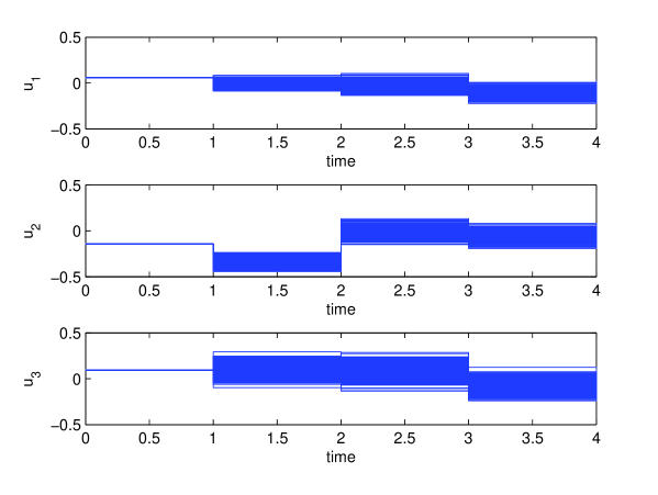
Refer to caption
Refer to caption
Figure 3: 1000 sample paths of the system with LQG control policy. Above: control input. Below: mass displacements.

We shall now introduce constraints on the state and the control input and study the feasibility of the problem with the methods of Section 3. The convex approximations to the chance-constrained optimization problems are solved numerically in Matlab by the toolbox CVX [18]. In all cases we shall compute a 555-stage affine optimal control policy and apply it to repeated runs of the system. Based on this we will discuss the feasibility of the hard constrained problem and the probability of constraint violation.

5.1 Polytopic constraints

Let us impose bounds on the control inputs, |u1(t)|0.1subscript𝑢1𝑡0.1|u_{1}(t)|\leq 0.1, |u2(t)|0.3subscript𝑢2𝑡0.3|u_{2}(t)|\leq 0.3 and |u3(t)|0.15subscript𝑢3𝑡0.15|u_{3}(t)|\leq 0.15, with t=0,,N1𝑡0𝑁1t=0,\ldots,N-1, and bounds on the mass displacements, |di(t)|10subscript𝑑𝑖𝑡10|d_{i}(t)|\leq 10, for i=1,,4𝑖14i=1,\cdots,4 and with t=1,,N𝑡1𝑁t=1,\ldots,N. In the notation of Section 3.2, these constraints are captured by the equation η(x¯,u¯)=Txx¯+Tuu¯y0𝜂¯𝑥¯𝑢superscript𝑇𝑥¯𝑥superscript𝑇𝑢¯𝑢𝑦0\eta(\bar{x},\bar{u})=T^{x}\bar{x}+T^{u}\bar{u}-y\leq 0 where Tx=[MT0]Tsuperscript𝑇𝑥superscriptmatrixsuperscript𝑀𝑇0𝑇T^{x}=\begin{bmatrix}M^{T}&0\end{bmatrix}^{T} and Tu=[0HT]Tsuperscript𝑇𝑢superscriptmatrix0superscript𝐻𝑇𝑇T^{u}=\begin{bmatrix}0&H^{T}\end{bmatrix}^{T}, with

M=[M1M1],M1=[I4×404×4I4×404×4],H=[II],formulae-sequence𝑀matrixsubscript𝑀1missing-subexpressionmissing-subexpressionmissing-subexpressionmissing-subexpressionmissing-subexpressionmissing-subexpressionsubscript𝑀1formulae-sequencesubscript𝑀1matrixsubscript𝐼44subscript044subscript𝐼44subscript044𝐻matrix𝐼𝐼M=\begin{bmatrix}M_{1}&&\\ &\ddots&\\ &&M_{1}\end{bmatrix},\quad M_{1}=\begin{bmatrix}I_{4\times 4}&0_{4\times 4}\\ -I_{4\times 4}&0_{4\times 4}\end{bmatrix},\quad H=\begin{bmatrix}I\\ -I\end{bmatrix},

and

y=[y1y2],y1=[1010],y2=[yy],y=[0.100.300.15].formulae-sequence𝑦matrixsubscript𝑦1subscript𝑦2formulae-sequencesubscript𝑦1matrix1010formulae-sequencesubscript𝑦2matrixsuperscript𝑦superscript𝑦superscript𝑦matrix0.100.300.15y=\begin{bmatrix}y_{1}\\ y_{2}\end{bmatrix},\quad y_{1}=\begin{bmatrix}10\\ \vdots\\ 10\end{bmatrix},\quad y_{2}=\begin{bmatrix}y^{\prime}\\ \vdots\\ y^{\prime}\end{bmatrix},\quad y^{\prime}=\begin{bmatrix}0.10\\ 0.30\\ 0.15\end{bmatrix}.

This hard constraint is relaxed to the probabilistic constraint [η(x¯,u¯)0]1αdelimited-[]𝜂¯𝑥¯𝑢01𝛼\mathbb{P}[\eta(\bar{x},\bar{u})\leq 0]\geq 1-\alpha. The resulting optimal control problem is then addressed by constraint separation  (Section 3.2.1) and ellipsoidal approximation (Section 3.2.2).

With constraint separation, the problem is feasible for α0.05𝛼0.05\alpha\geq 0.05. For α=0.1𝛼0.1\alpha=0.1, the application of the suboptimal control policy computed as in Proposition 6 yields the results shown in Figure 4.
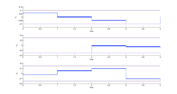
Refer to caption
Refer to caption
Figure 4: 1000 sample paths of the system with control policy computed via constraint separation. Above: control input. Below: mass displacements. Horizontal straight lines show bounds.

With this policy, the control input saturates within the required bounds whereas the mass displacements stay well below bounds. In fact, although the required probability of constraint satisfaction is 0.90.90.9, constraints were never violated in 1000 simulation runs. This suggests that the approximation incurred by constraint separation is quite conservative, mainly due to the relatively large number of constraints. It may also be noticed that the variability of the applied control input is rather small. This hints that the computed control policy is essentially open-loop, i.e. the linear feedback gain is small compared to the affine control term.

With the ellipsoidal approximation method, for the same probability level, the problem turns out to be infeasible, in accordance with the conclusions of Section 3.2.3. For the sake of investigation, we loosened the bounds on the mass displacements to |di(t)|100subscript𝑑𝑖𝑡100|d_{i}(t)|\leq 100 for all i𝑖i and t𝑡t. The problem of Proposition 7 is then feasible and the results from simulation of the controlled system are reported in Figure 5.
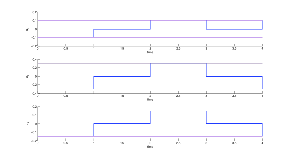
Refer to caption
Refer to caption
Figure 5: 1000 sample paths of the system with control policy computed via ellipsoidal approximation. Above: control input. Below: mass displacements. Horizontal straight lines show bounds.

Although the controller has been computed under much looser bounds, the control performance is similar to the one obtained with constraint separation, a clear sign that the ellipsoidal approximation is overly conservative in this case. Another evidence of inaccuracy is the fact that, while the control inputs get closer to the bounds, the magnitude of the displacements is not reduced. As in the case of constraint separation, the applied control input is insensitive to the specific simulation run, i.e. the control policy is essentially open loop.

5.2 Ellipsoidal constraints

Consider the constraint function

k=1N(d1(k)2+d2(k)2+d3(k)2+d4(k)2)+u¯2Ncsuperscriptsubscript𝑘1𝑁subscript𝑑1superscript𝑘2subscript𝑑2superscript𝑘2subscript𝑑3superscript𝑘2subscript𝑑4superscript𝑘2superscriptdelimited-∥∥¯𝑢2𝑁𝑐\sum_{k=1}^{N}\Bigl{(}d_{1}(k)^{2}+d_{2}(k)^{2}+d_{3}(k)^{2}+d_{4}(k)^{2}\Bigr{)}+\left\lVert{\bar{u}}\right\rVert^{2}\leq N\cdot c

with c=(12+12+12+12+0.12+0.152+0.32)=4.1225𝑐superscript12superscript12superscript12superscript12superscript0.12superscript0.152superscript0.324.1225c=(1^{2}+1^{2}+1^{2}+1^{2}+0.1^{2}+0.15^{2}+0.3^{2})=4.1225. Unlike the previous section, we do not impose bounds on di(k)subscript𝑑𝑖𝑘d_{i}(k) and ui(k)subscript𝑢𝑖𝑘u_{i}(k) at each k𝑘k but instead require that the total “spending” on x𝑥x and u𝑢u does not exceed a total “budget”. This constraint can be modelled in the form of Section 3.3, namely

η(x¯,u¯)=([x¯u¯]δ)TΞ([x¯u¯]δ)10,𝜂¯𝑥¯𝑢superscriptmatrix¯𝑥¯𝑢𝛿𝑇Ξmatrix¯𝑥¯𝑢𝛿10\eta(\bar{x},\bar{u})=\Biggl{(}\begin{bmatrix}\bar{x}\\ \bar{u}\end{bmatrix}-\delta\Biggr{)}^{T}\Xi\Biggl{(}\begin{bmatrix}\bar{x}\\ \bar{u}\end{bmatrix}-\delta\Biggr{)}-1\leq 0,

with δ=0𝛿0\delta=0 and Ξ=1Nc[L00I]Ξ1𝑁𝑐matrix𝐿00𝐼\Xi=\frac{1}{N\cdot c}\begin{bmatrix}L&0\\ 0&I\end{bmatrix}, where

L=[L1L1],L1=[I4×404×404×404×4].formulae-sequence𝐿matrixsubscript𝐿1missing-subexpressionmissing-subexpressionmissing-subexpressionmissing-subexpressionmissing-subexpressionmissing-subexpressionsubscript𝐿1subscript𝐿1matrixsubscript𝐼44subscript044subscript044subscript044L=\begin{bmatrix}L_{1}&&\\ &\ddots&\\ &&L_{1}\end{bmatrix},L_{1}=\begin{bmatrix}I_{4\times 4}&0_{4\times 4}\\ 0_{4\times 4}&0_{4\times 4}\end{bmatrix}.

The constrained control policy for N=5𝑁5N=5 and α=0.1𝛼0.1\alpha=0.1 is computed by solving the LMI problem of Proposition 11. Results from simulations of the closed-loop system are reported in Figure 6. Once again, constraints were not violated over 1000 simulated runs, showing the conservatism of the approximation. It is interesting to note that the displacements of the masses are generally smaller than those obtained by the controller computed under affine constraints, at the cost of a slightly more expensive control action. In contrast with the affine constraints case, the control action obtained here is much more sensitive to the noise in the dynamics, i.e. the feedback action is more pronounced.
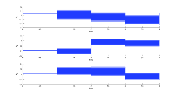
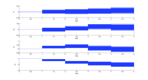
Refer to caption
Refer to caption
Figure 6: 1000 sample paths of the system with control policy computed via ellipsoidal constraints. Above: control input. Below: mass displacements. Horizontal straight lines show bounds.

6 Conclusions

We have studied the convexity of optimization problems with probabilistic constraints arising in model predictive control of stochastic dynamical systems. We have given conditions for the convexity of expectation-type objective functions and constraints. Convex approximations have been derived for nonconvex probabilistic constraints. Results have been exemplified by a numerical simulation study.

Open issues that will be addressed in the future are the role of the tunable parameters (e.g. the αisubscript𝛼𝑖\alpha_{i} in Section 3.2.1, the tisubscript𝑡𝑖t_{i} of Section 3.2.4 and the βisubscript𝛽𝑖\beta_{i} in Section 4) in the various optimization problems, and the effect of different choices of the ICC functions φisubscript𝜑𝑖\varphi_{i} (Section 4). Directions of future research also include the extension of the results presented here to the case of noisy state measurements, the exact or approximate solution of the stochastic optimization problems in terms of explicit control laws and the control of stochastic systems with probabilistic constraints on the state via bounded control laws.

References

  • [1] M. Agarwal, E. Cinquemani, D. Chatterjee, and J. Lygeros, On convexity of stochastic optimization problems with constraints, in Proceedings of the European Control Conference (ECC’09), 2009. Accepted.
  • [2] J. M. Alden and R. L. Smith, Rolling horizon procedures in nonhomogeneous Markov decision processes, Operations Research, 40 (1992), pp. S183–S194.
  • [3] K. Åström, Introduction to Stochastic Control Theory, Academic Press, New York, 1970.
  • [4] I. Batina, Model predictive control for stochastic systems by randomized algorithms, PhD thesis, Technische Universiteit Eindhoven, 2004.
  • [5] A. Ben-Tal, S. Boyd, and A. Nemirovski, Extending scope of robust optimization, Mathematical Programming, 107 (2006), pp. 63–89.
  • [6] A. Ben-Tal, A. Goryashko, E. Guslitzer, and A. Nemirovski, Adjustable robust solutions of uncertain linear programs, Mathematical Programming, 99 (2004), pp. 351–376.
  • [7] D. P. Bertsekas, Dynamic programming and suboptimal control: A survey from ADP to MPC, European Journal of Control, 11 (2005).
  • [8] D. Bertsimas and D. B. Brown, Constrained stochastic LQC: a tractable approach, IEEE Transactions on Automatic Control, 52 (2007), pp. 1826–1841.
  • [9] D. Bertsimas and M. Sim, Tractable approximations to robust conic optimization problems, Mathematical Programming, 107 (2006), pp. 5–36.
  • [10] V. I. Bogachev, Gaussian Measures, vol. 62 of Mathematical Surveys and Monographs, American Mathematical Society, Providence, RI, 1998.
  • [11] S. Boyd and L. Vandenberghe, Convex Optimization, Cambridge University Press, Cambridge, 2004.
  • [12] D. Chatterjee, E. Cinquemani, G. Chaloulos, and J. Lygeros, Stochastic control up to a hitting time: optimality and rolling-horizon implementation. http://arxiv.org/abs/0806.3008, jun 2008.
  • [13] D. Chatterjee, E. Cinquemani, and J. Lygeros, Maximizing the probability of attaining a target prior to extinction. http://arxiv.org/abs/0904.4143, apr 2009.
  • [14] D. Chatterjee, P. Hokayem, and J. Lygeros, Stochastic model predictive control with bounded control inputs: a vector space approach. http://arxiv.org/abs/0903.5444, mar 2009.
  • [15] P. D. Couchman, M. Cannon, and B. Kouvaritakis, Stochastic MPC with inequality stability constraints, Automatica J. IFAC, 42 (2006), pp. 2169–2174.
  • [16] R. M. Dudley, Real Analysis and Probability, vol. 74 of Cambridge Studies in Advanced Mathematics, Cambridge University Press, Cambridge, 2002. Revised reprint of the 1989 original.
  • [17] P. J. Goulart, E. C. Kerrigan, and J. M. Maciejowski, Optimization over state feedback policies for robust control with constraints, Automatica, 42 (2006), pp. 523–533.
  • [18] M. Grant and S. Boyd, CVX: Matlab software for disciplined convex programming, feb 2009. (web page and software) http://stanford.edu/similar-to\simboyd/cvx.
  • [19] W. K. K. Haneveld, On integrated chance constraints, in Stochastic programming (Gargnano), vol. 76 of Lecture Notes in Control and Inform. Sci., Springer, Berlin, 1983, pp. 194–209.
  • [20] W. K. K. Haneveld and M. H. van der Vlerk, Integrated chance constraints: reduced forms and an algorithm, Computational Management Science, 3 (2006), pp. 245–269.
  • [21] J. Löfberg, Minimax Approaches to Robust Model Predictive Control, PhD thesis, Linköping Universitet, Apr 2003.
  • [22] J. Maciejowski, Predictive Control with Constraints, Prentice Hall, 2002.
  • [23] A. Nemirovski and A. Shapiro, Convex approximations of chance constrained programs, SIAM Journal on Control and Optimization, 17 (2006), pp. 969–996.
  • [24] A. Prékopa, Stochastic Programming, vol. 324 of Mathematics and its Applications, Kluwer Academic Publishers Group, Dordrecht, 1995.
  • [25] J. Primbs, A soft constraint approach to stochastic receding horizon control, in Proceedings of the 46th IEEE Conference on Decision and Control, 2007, pp. 4797 – 4802.
  • [26] J. Primbs, Stochastic receding horizon control of constrained linear systems with state and control multiplicative noise, in Proceedings of the 26th American Control Conference, 2007.
  • [27] G. C. R. Tempo and F. Dabbene, Randomized Algorithms for Analysis and Control of Uncertain Systems, Springer-Verlag, 2005.
  • [28] J. Spall, Introduction to Stochastic Search and Optimization: Estimation, Simulation, and Control, Wiley, Hoboken, NJ, 2003.
  • [29] D. H. van Hessem and O. H. Bosgra, A full solution to the constrained stochastic closed-loop mpc problem via state and innovations feedback and its receding horizon implementation, in Proceedings of the 42nd IEEE Conference on Decision and Control, vol. 1, 9-12 Dec. 2003, pp. 929–934.
  • [30] M. Vidyasagar, Randomized algorithms for robust controller synthesis using statistical learning theory, Automatica, 37 (2001), pp. 1515–1528.