A parametrization for the growth index of linear matter perturbations

Abstract

We propose a parametrization for the growth index of the linear matter perturbations, $\gamma(z)=\gamma_{0}+\frac{z}{1+z}\gamma_{1}$. The growth factor of the perturbations parameterized as $\Omega_{m}^{\gamma}$ is analyzed for both the $w$CDM model and the DGP model with our proposed form for $\gamma$. We find that $\gamma_{1}$ is negative for the $w$CDM model but is positive for the DGP model. Thus it provides another signature to discriminate them. We demonstrate that $\Omega_{m}^{\gamma}$ with $\gamma$ taking our proposed form approximates the growth factor very well both at low and high redshfits for both kinds of models. In fact, the error is below $0.03\%$ for the $\Lambda$CDM model and $0.18\%$ for the DGP model for all redshifts when $\Omega_{m0}=0.27$. Therefore, our parametrization may be robustly used to constrain the growth index of different models with the observational data which include points for redshifts ranging from 0.15 to 3.8, thus providing discriminative signatures for different models.

I Introduction

The growing observational evidences Sne ; CMB ; SDSS show that the present expansion of our universe is accelerating. Basically, two kinds of physical models have been proposed to explain this mysterious phenomenon. One is dark energy, which has a sufficient negative pressure to induce a late-time accelerated expansion; the other is the modified gravity, which originates from the idea that our understanding to gravity is incorrect in the cosmic scale and general relativity needs to be modified. However, many different models proposed so far share the same late time cosmological expansion, therefore an important task is to discriminate them to determine which one correctly describes the whole evolution of the universe. Recently, some attempts have been made r12 ; r13 ; r14 ; r15 ; r16 ; r17 in this regard. A particular effort to discriminate different models focuses on the growth function $\delta(z)\equiv\delta\rho_{m}/\rho_{m}$ of the linear matter density contrast as a function of redshift $z$  Starobinsky1998 ; Huterer2007 ; Sereno2006 ; Knox2006 ; Ishak2006 ; Acquaviva2008 ; Daniel2008 ; Sapone2007 ; Ballesteros2008 ; Bertschinger2008 ; Laszlo2008 ; kunz2007 ; Kiakotou2008 ; Linder2007 ; Wei2008 ; Wei20082 ; Linder2005 ; Amendola ; Nesseris2008 ; Wang2008 ; Boisseau2000 ; Gong2008 ; Gong2009 ; Polarski2008 ; Gannouji2008 ; Gannouji20082 ; Fu2009 , where $\rho_{m}$ is the energy density of matter. While different models give the same late time expansion, they may produce different growth of matter perturbations Starobinsky1998 .

In order to discriminate different models using the matter perturbations, the growth factor $f\equiv\frac{d\ln\delta}{d\ln a}$ is used. In Ref. Fry1985 , the authors found that this growth factor can be parameterized as

$$f=\Omega_{m}^{\gamma},$$ (1)

where $\gamma$ is called the growth index and $\Omega_{m}$ is the fractional energy density of matter. Using the fact that $\Omega_{m}\simeq 1$ at the high redshift, treating $\gamma$ as a constant and expanding, around $\Omega_{m}=1$, the equation obtained by submitting the above expression into the equation of $f$ (Eq. (4) below), one can easily obtain the theoretical values of $\gamma$ for different models. For example, the theoretical values of $\gamma$ for the $\Lambda$CDM model and the Dvali-Gabadadze-Porrati (DGP) brane-world model Dvali2000 are $\gamma_{\infty}=6/11$ Linder2007 ; Linder2005 and $\gamma_{\infty}=11/16$ Linder2007 ; Wei2008 , respectively. Thus if the value of $\gamma$ can be determined by observations, one can discriminate these models. Theoretically, if $\gamma$ can be treated as a constant and the value of $\Omega_{m,0}$ is known, we can also determine the value of $\gamma$ at $z=0$. This actually gives a better approximation to $f$ as will be shown later. However, the fact that we do not have a precise value of $\Omega_{m,0}$ from observations restricts our ability to obtain an exact value of constant $\gamma$. Recently by comparing $\Omega^{\gamma_{\infty}}$ with $f$, the author in Ref. Gong2008 found the error is nearly zero at the high redshift, but at low redshift, with $\Omega_{m,0}=0.27$, the error is larger than $1.2\%$ for $\Lambda$CDM model and $3\%$ for the DGP model. The discrepancy originates from the fact that in general $\gamma$ is not a constant but should be a function of redshift, especially at low redshift region ($z<2$). Therefore, if one wants to discriminate different models by using the current observational data on the matter perturbations with $\gamma$ being taken as a constant, then the results may be biased, since there are about half of growth factor data points at the redshift region $z<2$ Tegmark2006 .

So, it seems necessary to consider an evolutionary growth index $\gamma(z)$. In this regard the authors in Refs. Polarski2008 ; Gannouji2008 ; Gannouji20082 ; Fu2009 studied $\gamma(z)$ with a linear expansion, $\gamma\approx\gamma_{0}+\gamma_{0}^{\prime}z$, and found for different models the $\gamma_{0}^{\prime}$ is different, which may provide another signature to discriminate different models. Certainly this linear expansion gives a very good approximation at $z<0.5$, but it is invalid at high redshift region and thus is not usable for discriminating different models by constraining $\gamma_{0}$ and $\gamma_{0}^{\prime}$ from current observations, since there are few growth factor data points at $z<0.5$. In Ref. Gong2008 the author considered the correction to $\gamma$ by introducing an $\Omega_{m}-1$ term and found that, with $\Omega_{m,0}=0.27$, the error is blow $0.25\%$ for the $\Lambda$CDM model and below $0.4\%$ for the DGP model, which are less than those obtained in the case of a constant $\gamma=\gamma_{\infty}$. However, principally speaking, this correction cannot be extended to low redshift where the deviation of $\Omega_{m}$ from $1$ is very large. Therefore, it is desirable to have a new form of $\gamma(z)$, which is applicable to all the observational data and can, at the same time, give a very good approximation to $f$. In this paper we propose a parameterized form on $\gamma(z)$

$$\gamma(z)=\gamma_{0}+\gamma_{1}{z\over 1+z}.$$ (2)

By numerical calculations, we will demonstrate that this parametrization can approximate $f$ very well at both low and high redshifts for both the $w$CDM model and the DGP model, and as a result, it is applicable to all the data points and can be used to better discriminate these models using observational data.

II the $w$CDM model

In this section, the dark energy model with a constant equation of state ($w$CDM) is studied. To the linear order of matter perturbations, the growth function $\delta(z)$ at scales much smaller than the Hubble radius obeys the following equation

$$\ddot{\delta}+2H\dot{\delta}-4\pi G_{eff}\,\rho_{m}\delta=0,$$ (3)

where $G_{eff}$ is an effective Newton gravity constant and the dot denotes the derivative with respect to the time $t$. Using the growth factor $f\equiv d\ln\delta/d\ln a$, the above equation becomes

$${d\;f\over d\ln a}+f^{2}+\left(\frac{\dot{H}}{H^{2}}+2\right)f=\frac{3}{2}\frac{G_{eff}}{G_{N}}\Omega_{m}.$$ (4)

For the $w$CDM dark energy model, the above equation can be reexpressed as

$$3w\Omega_{m}(1-\Omega_{m})\frac{df}{d\Omega_{m}}+f^{2}+\left[\frac{1}{2}-\frac{3}{2}w(1-\Omega_{m})\right]f=\frac{3}{2}\Omega_{m}\,,$$ (5)

where ${G_{eff}\over G_{N}}=1$ is used. In general, it is hard to obtain an analytical solution to the above equation and we need to resort to numerical methods. In fact, the equation can be solved numerically by taking into account the condition that $f=1$ at the high redshift since $\Omega_{m}=1$ at $z>>1$. Using the Eq. (1), one can get

$$-(1+z)\gamma^{\prime}\ln{\Omega_{m}}+\Omega_{m}^{\gamma}+{1\over 2}[1+3w(2\gamma-1)(1-\Omega_{m})]={3\over 2}\Omega_{m}^{1-\gamma}\;.$$ (6)

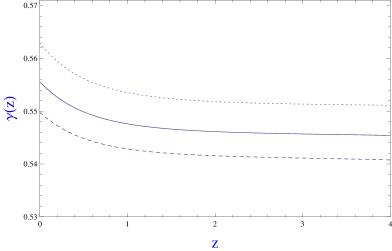
This equation is also very hard to be solved analytically. Fortunately using the relation $f=\Omega_{m}^{\gamma(z)}$, we can obtain the evolution of $\gamma(z)$ with the redshift, which is shown in Fig. (1) for $w$CDM model with different values of $w$. It is easy to see that $\gamma(z)$ can not be regarded as a constant especially at the redshift region ($z<2$) where some the observational data points are obtained. Therefore it is obviously unreliable to discriminate different models with these observational data while treating the growth index $\gamma$ as a constant.

Now let us examine if our proposed form of parametrization, Eq. (2), gives a good approximation to the growth factor $f$. If we prior know the value of $\Omega_{m,0}$, and find the value of $\gamma_{0}$ through $f_{0}$ obtained by numerically solving solution Eq. (5), then by substituting Eq. (2) into Eq. (6), we get an expression for $\gamma_{1}$ which yields a different value for a different redshift $z$. This is because our proposed parameterized form of $\gamma(z)$ is not an exact solution but only gives an approximation to the curve shown in Fig. (1). To see how well our approximation is, let us take, for simplicity, the value of $\gamma_{1}$ at the $z=0$,

$$\gamma_{1}=({\,\ln\Omega_{m,0}^{-1}}\,)^{-1}\bigg{[}{3\over 2}\Omega_{m,0}^{1-\gamma_{0}}-\Omega_{m,0}^{\gamma_{0}}-{3\over 2}w(2\gamma_{0}-1)(1-\Omega_{m,0})-{1\over 2}\bigg{]}\;,$$ (7)

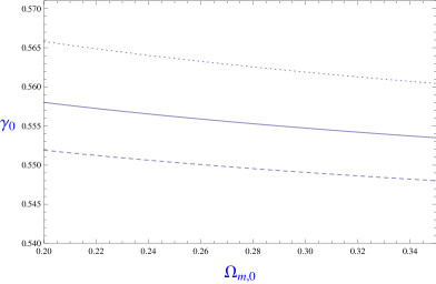
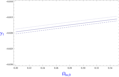
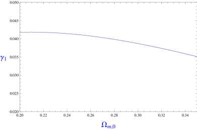
which is determined by the values $\Omega_{m,0}$ and $\gamma_{0}$. Since the value of $\Omega_{m,0}$ can be determined by the observations and $\gamma_{0}$ can be obtained by the numerical solution of $f$ with the relation $f_{0}=\Omega_{m,0}^{\gamma_{0}}$, we can get the value of $\gamma_{1}$. In Fig. (2), we show the allowed region of $\gamma_{0}$ and the corresponding $\gamma_{1}$ with a prior given region of $\Omega_{m,0}$: $0.20\leq\Omega_{m,0}\leq 0.35$. From this Figure we can see that $\gamma_{0}$ and $\gamma_{1}$ vary only slightly as $\Omega_{m,0}$ changes.

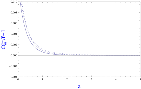
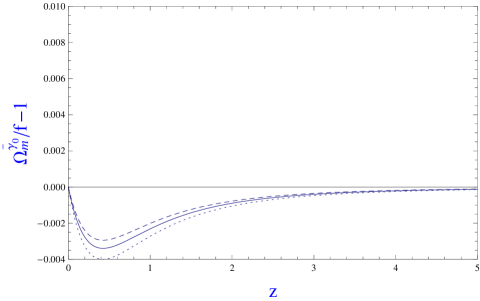
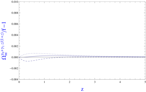
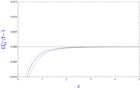
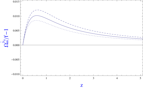
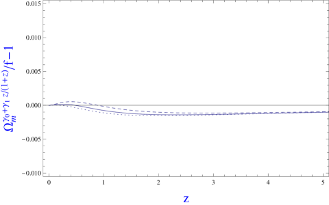
Now we discuss how well $\Omega_{m}^{\gamma}$, with $\gamma$ taking our parameterized form, approximates the growth factor $f$. Numerical results are shown in Fig. (3). Three different cases are plotted for comparison. One is that the growth index is treated as a constant which is determined at very high redshift where $\Omega_{m}=1$ ($\gamma_{\infty}$). This case is shown on the upper panel. The second is that $\gamma$ is also treated as a constant but the constant is obtained at $z=0$ denoted as $\overline{\gamma}_{0}$ with $\overline{\gamma}_{0}=\ln f(0)/\ln\Omega_{m,0}(0)$. The result is shown in the middle panel. From the Figure, one can see that $\Omega_{m}^{\gamma}$ with a constant $\gamma$ given by $\overline{\gamma}_{0}$ approximates $f$ better at low redshifts than that given by $\gamma_{\infty}$, but is not as good at high redshifts ($z>1$). This is because $\overline{\gamma}_{0}$ is a good approximation at the low redshift while $\gamma_{\infty}$ gives a good approximation at the high redshift. The third is that $\gamma$ is evolving with redshift and takes our proposed form given in Eq. (2). The result is shown in the bottom panel. Now $\Omega_{m}^{\gamma}$ approximates $f$ very well both at low and high redshfits, and remarkably it approximates $f$ better than $0.08\%$ even at low redshfits. Notice, however, that for $\Omega_{m}^{\gamma_{\infty}}$ the error is over $1\%$ at low redshifts and for $\Omega_{m}^{\overline{\gamma}_{0}}$ the largest error is $0.4\%$. For the case of $w=-1$ ($\Lambda$CDM), we find that the error resulting from using our proposed form is below $0.03\%$. This is much less than that, obtained in Ref. Gong2008 , for $\Omega_{m}^{\gamma}$ with corrections to a constant $\gamma_{\infty}$ added through expanding $\gamma$ at $\Omega_{m}=1$ as $\gamma=\gamma_{\infty}+\frac{15}{1331}(1-\Omega_{m})$, where the error is only blow $0.25\%$. We get approximately one order of magnitude improvement in terms of errors in the approximation. Therefore, the form given in Eq. (2) is basically very close to the real evolution of $\gamma$ with redshift.

III the DGP model

Now we will discuss a modified gravity model, the DGP model. For this model, the effective Newton constant takes the following form

$${G_{\rm eff}\over G_{N}}=\frac{2(1+2\Omega_{m})}{3(1+\Omega_{m}^{2})}.$$ (8)

According to Refs. Wei2008 ; Gong2009 ; Lue2004 ; Koyma2006 , the growth factor $f$ satisfies the equation

$$-3\frac{(1-\Omega_{m})\Omega_{m}}{1+\Omega_{m}}{df\over d\Omega_{m}}+f^{2}+f\frac{2-\Omega_{m}}{1+\Omega_{m}}=\frac{\Omega_{m}(1+2\Omega_{m}^{2})}{1+\Omega_{m}^{2}}.$$ (9)

Submitting Eq. (1) into the above equation, we can obtain an equation of $\gamma(z)$

$${1\over 2}\bigg{[}1-\frac{3(1-\Omega_{m})}{1+\Omega_{m}}(2\gamma-1)\bigg{]}-(1+z)\gamma^{\prime}\ln{\Omega_{m}}+\Omega_{m}^{\gamma}=\frac{1+2\Omega_{m}^{2}}{1+\Omega_{m}^{2}}\Omega_{m}^{1-\gamma}\,.$$ (10)

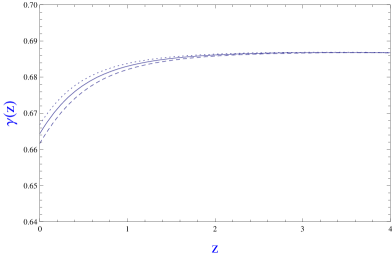
The numerical solution for $\gamma(z)$ is shown in Fig. (4) with different values of $\Omega_{m,0}$. From Figure, one can see that the $\gamma(z)$ is evolutionary especially at low redshifts ($z<2$) and is an increasing function of redshift, in contrast to the $w$CDM model, where $\gamma(z)$ is a decreasing one. Now, one can show that $\gamma_{1}$ determined at $z=0$ is given

$$\gamma_{1} = (\ln\Omega_{m,0}^{-1})^{-1}\bigg{[}-\Omega_{m,0}^{\gamma_{0}}+\frac{1+2\Omega_{m,0}^{2}}{1+\Omega_{m,0}^{2}}\Omega_{m,0}^{1-\gamma_{0}}-{1\over 2}+\frac{3(1-\Omega_{m,0})}{1+\Omega_{m,0}}(\gamma_{0}-{1\over 2})\bigg{]}\,.$$ (11)

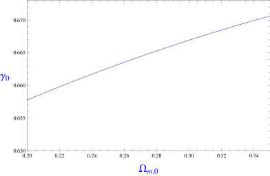
In Fig. (5) we plot the possible region of $\gamma_{0}$ and $\gamma_{1}$ for $0.20\leq\Omega_{m,0}\leq 0.35$. It is easy to see that $\gamma_{0}$ increases from $0.658$ to $0.671$ and $\gamma_{1}$ decreases from $0.042$ to $0.035$. Apparently $\gamma_{1}$ here is positive, whereas $\gamma_{1}(\approx-0.02)$ in the $w$CDM model is negative. Therefore, $\gamma_{1}$ also provides a signature to discriminate the DGP model and the $w$CDM model.

How well the $\Omega_{m}^{\gamma}$ approximate the growth factor $f$ is discussed as done in above section and the results are shown in Fig. (6). Comparing the upper and middle panels of this figure, we find, as in the $w$CDM model, that $\Omega_{m}^{\gamma}$ with constant $\gamma$ given by $\overline{\gamma}_{0}$ approximates $f$ better at low redshifts than that given by $\gamma_{\infty}$, but is not as good at high redshifts ($z>1$). Comparing these two panels with the bottom one, one sees that at low redshifts $\gamma(z)$ proposed in the present paper gives the best approximation. At low redshifts, the error using our proposed form for $\gamma(z)$ is blow $0.2\%$ , but for a constant $\gamma$, the error is larger than $2\%$ when $\gamma=\gamma_{\infty}$ and is only blow $1.2\%$ when $\gamma=\overline{\gamma}_{0}$. At low redshifts, the approximation with our proposed form is also better than that obtained in Ref. Gong2008 where the constant $\gamma$ is corrected as $\gamma=\gamma_{\infty}+\frac{7}{5632}(1-\Omega_{m})$, since, when $\Omega_{m,0}=0.27$, the error of our proposed form is blow $0.18\%$ while it is only blow $0.25\%$ for $\gamma$ corrected with a $1-\Omega_{m}$ term. It is worthy to note that $\Omega_{m}^{\gamma(z)}$ with $\gamma(z)$ taking our proposed form still approximates $f$ very well for all redshifts, since the largest error is only $0.18\%$, when $\Omega_{m,0}=0.27$.

IV Conclusion

In this paper, we propose a parameterized form for the growth index of the linear matter perturbations, $\gamma(z)=\gamma_{0}+\frac{z}{1+z}\gamma_{1}$. The growth factor of the linear matter perturbations is analyzed for both the $w$CDM model and the DGP model. We find that $\gamma_{1}$ is negative for the $w$CDM model but is positive for the DGP model. Thus it provides another signature to discriminate them. If we parameterize the growth factor $f$ as $\Omega_{m}^{\gamma}$, then at low redshifts, $\Omega_{m}^{\gamma}$ with $\gamma$ taking our proposed form approximates the growth factor $f$ better than that in the case of a constant $\gamma$ with or without the $1-\Omega_{m}$ correction term. At high redshifts, the approximation is also very good. In fact, the error is below $0.03\%$ for the $\Lambda$CDM model and $0.18\%$ for the DGP model for all redshifts when $\Omega_{m0}=0.27$. Therefore, our parametrization can be robustly used to constrain the growth index of different models with the observational data which include points for redshifts ranging from 0.15 to 3.8, thus providing discriminative signatures for different models.

Figure 1: The evolution of growth index $\gamma(z)$ with redshift for the $w$CDM model with $\Omega_{m,0}=0.27$. The solid, dashed and dotted curves correspond to $w=-1$, $-0.8$ and $-1.2$ respectively.

Figure 2: The allowed regions of $\gamma_{0}$ and $\gamma_{1}$ for the $w$CDM model with $0.2\leq\Omega_{m,0}\leq 0.35$. The solid, dashed and dotted curves correspond to $w=-1$, $-0.8$ and $-1.2$ respectively.

Figure 3: The relative difference between the growth factor $f$ and $\Omega_{m}^{\gamma}$ for the $w$CDM model with $\Omega_{m,0}=0.27$. The upper, middle and bottom panels show the results of $\gamma=\gamma_{\infty}$, $\overline{\gamma}_{0}$ and $\gamma=\gamma_{0}+z/(1+z)\gamma_{1}$, respectively. The solid, dashed, and dotted curves show the results for $w=-1$, $-0.8$ and $-1.2$, respectively.

Figure 4: The evolution of growth index $\gamma(z)$ with the redshift for the DGP model. The solid, dashed and dotted curves correspond to $\Omega_{m,0}=0.27$, $0.24$ and $0.30$ respectively.

Figure 5: The allowed regions of $\gamma_{0}$ and $\gamma_{1}$ for the DGP model with $0.2\leq\Omega_{m,0}\leq 0.35$.

Figure 6: The relative difference between the growth factor $f$ and $\Omega_{m}^{\gamma}$ for the DGP model. The upper, middle and bottom panels show the results of $\gamma=\gamma_{\infty}$, $\overline{\gamma}_{0}$ and $\gamma=\gamma_{0}+z/(1+z)\gamma_{1}$, respectively. The solid, dashed, and dotted curves show the results for $\Omega_{m,0}=0.27$, $0.24$ and $0.30$, respectively.

References

- (1) A. G. Riess, A. V. Filippenko, P. Challis, et al., Astron. J. 116, 1009 (1998); S. J. Perlmutter, G. Aldering, G. Goldhaber, et al., Astrophy. J. 517, 565 (1999); J. L. Tonry et al., Astrophys. J. 594, 1 (2003); R. A. Knop et al., Astrophys. J. 598, 102 (2003); A. G. Riess et al., Astrophys. J. 607, 665 (2004); A. G. Riess et al., Astrophys. J. 659, 98 (2007); P. Astier et al., Astron. Astrophys. 447, 31 (2006); J. D. Neill et al., Astron. J. 132, 1126 (2006); W. M. Wood-Vasey et al., Astrophys. J. 666, 694 (2007); T. M. Davis et al., Astrophys. J. 666, 716 (2007).
- (2) D. N. Spergel, et al., Astrophys. J. Suppl. 170, 377 (2007); L. Page, et al., Astrophys. J. Suppl. 170, 335 (2007); G. Hinshaw, et al., Astrophys. J. Suppl. 170, 288 (2007); N. Jarosik, et al., Astrophys. J. Suppl. 170, 263 (2007).
- (3) D. J. Eisenstein, et al., Astorphys. J. 633, 560 (2005); E. Komatsu, et al., Astrophys. J. Suppl. 180, 330 (2009).
- (4) R. R. Caldwell and E. V. Linder, Phys. Rev. Lett. 95, 141301 (2005); E. V. Linder, Phys. Rev. D 73, 063010 (2006).
- (5) R. J. Scherrer, Phys. Rev. D 73, 043502 (2006).
- (6) T. Chiba, Phys. Rev. D 73, 063501 (2006).
- (7) E. V. Linder, Gen. Rel. Grav. 40, 329 (2008).
- (8) V. Sahni, T. D. Saini, A. A. Starobinsky and U. Alam, JETP Lett. 77, 201 (2003); U. Alam, V. Sahni, T. D. Saini and A. A. Starobinsky, Mon. Not. Roy. Astron. Soc. 344, 1057 (2003).
- (9) H. Wei and R. G. Cai, Phys. Lett. B 655, 1 (2007).
- (10) A. A. Starobinsky, JETP Lett. 68, 757 (1998).
- (11) D. Huterer and E. V. Linder, Phys. Rev. D 75, 023519 (2007).
- (12) M. Sereno and J. A. Peacock, Mon. Not. Roy. Astron. Soc. 371, 719 (2006).
- (13) L. Knox, Y.-S. Song and J. A. Tyson, Phys. Rev. D 74, 023512 (2006).
- (14) M. Ishak, A. Upadhye and D. N. Spergel, Phys. Rev. D 74, 043513 (2006).
- (15) V. Acquaviva, A. Hajian, D. N. Spergel and S. Das, Phys. Rev. D 78, 043514 (2008).
- (16) T. Koivisto and D. F. Mota, Phys. Rev. D 73 (2006) 083502; D. F. Mota, J. R. Kristiansen, T. Koivisto and N. E. Groeneboom Mon.Not.Roy.Astron.Soc. 382 (2007) 793; S. Daniel, R. Caldwell, A. Cooray and A. Melchiorri, Phys. Rev. D 77, 103513 (2008).
- (17) D. Sapone and L. Amendola, arXiv: 0709.2792.
- (18) G. Ballesteros and A. Riotto, Phys. Lett. B 668, 171 (2008).
- (19) E. Bertschinger and P. Zukin, Phys. Rev. D 78, 024015 (2008).
- (20) I. Laszlo and R. Bean, Phys. Rev. D 77, 024048 (2008).
- (21) M. Kunz and D. Sapone, Phys. Rev. Lett. 98, 121301 (2007).
- (22) A. Kiakotou, O Elgaro and O. Lahav, Phys. Rev. D 77, 063005 (2008).
- (23) E. V. Linder and R. N. Cahn, Astropart. Phys. 28, 481 (2007).
- (24) H. Wei, Phys. Lett. B 664, 1 (2008).
- (25) H. Wei, S. N. Zhang, Phys. Rev. D 78, 023011 (2008).
- (26) Y. Gong, Phys. Rev. D 78, 123010 (2008).
- (27) Y. Gong, M. Ishak and A. Wang, arXiv: 0903.0001.
- (28) E. V. Linder, Phys. Rev. D 72, 043529 (2005).
- (29) C. Di Porto and L. Amendola, Phys. Rev. D 77, 083508 (2008); L. Amendola, M. Kunz and D. Sapone, arXiv: 0704.2421.
- (30) S. Nesseris and L. Perivolaropoulos, Phys. Rev. D 77, 023504 (2008).
- (31) Y. Wang, J. Cosmol. Astropart. Phys. 5, 21 (2008).
- (32) B. Boisseau, G. Esposito-Far se, D. Polarski, A. A. Starobinsky, Phys. Rev. Lett. 85, 2236 (2000); M.J. Mortonson, W. Hu and D. Huterer, Phys. Rev. D 79 (2009) 023004; J. He, B. Wang, Y. P. Jing, arXiv:0902.0660; J. B. Dent, S. Dutta and L. Perivolaropoulos, arXiv:0903.5296; M. Ishak and J. Dossett, arXiv:0905.2470.
- (33) D. Polarski and R. Gannouji, Phys. Lett. B 660, 439 (2008).
- (34) R. Gannouji and D. Polarski, J. Cosmol. Astropart. Phys. 05, 018 (2008).
- (35) R. Gannouji, B. Moraes and D. Polarski, arXiv: 0809.3374.
- (36) X. Fu, P. Wu and H. Yu, Physics Letters B 677 (2009) 12
- (37) J. N. Fry, Phys. Lett. B 158, 211 (1985); A. P. Lightman and P. L. Schechter, Astrophys. J. 74, 831 (1990); L. Wang and P. J. Steinhardt, Astrophys. J. 508, 483 (1998);
- (38) G. Dvali, G. Gabadadze and M. Porrati, Phys. Lett. B 485, 208 (2000); Z. Zhu, M. Sereno, Astro. Astrophys. 487, 831 (2008).
- (39) L. Guzzo et al., Nature 451, 541 (2008). M. Tegmark el al., Phys. Rev. D 74, 123507 (2006); N. P. Ross et al., Mont. Not. R. Astron. Soc. 381, 573 (2007); J. da Angela et al., Mont. Not. R. Astron. Soc. 383, 565 (2008); P. McDonald et al., Astrophys. J. 635, 761 (2005); M. Viel, M. G. Haehnelt and V. Springel, Mont. Not. R. Astron. Soc. 354, 684 (2004); M. Viel, M. G. Haehnelt and V. Springel, Mont. Not. R. Astron. Soc. 365, 231 (2006).
- (40) A. Lue, R. Scoccimarro and G. D. Starkman, Phys. Rev. D 69, 124015 (2004).
- (41) K. Koyama and R. Maartens, J. Cosmol. Astropart. Phys. 01, 016 (2006).