Scaling of loop-erased walks in 2 to 4 dimensions

Abstract

We simulate loop-erased random walks on simple (hyper-)cubic lattices of dimensions 2, 3 and 4. These simulations were mainly motivated to test recent two loop renormalization group predictions for logarithmic corrections in $d=4$, simulations in lower dimensions were done for completeness and in order to test the algorithm. In $d=2$, we verify with high precision the prediction $D=5/4$, where the number of steps $n$ after erasure scales with the number $N$ of steps before erasure as $n\sim N^{D/2}$. In $d=3$ we again find a power law, but with an exponent different from the one found in the most precise previous simulations: $D=1.6236\pm 0.0004$. Finally, we see clear deviations from the naive scaling $n\sim N$ in $d=4$. While they agree only qualitatively with the leading logarithmic corrections predicted by several authors, their agreement with the two-loop prediction is nearly perfect.

I Introduction

The loop-erased random walk (LERW) is one of the simplest critical phenomena. It has no direct physical realization, although it is related to several well studied problems in statistical physics Majumdar ; Duplantier ; Schramm . It was first studied by Lawler Lawler as a simplified version of self avoiding walks. It is defined by performing a standard random walk, and erasing any loop as soon as it is formed. Thus it has no self-intersections, but it has different statistics from the usual self avoiding walk (SAW) where the entire walk is erased as soon as a loop is formed.

Since there is no attrition for the LERW, the entropic critical exponent (called $\gamma$ for SAWs) is trivially equal to 1, and any scaling behavior refers to geometric quantities. Let us denote by $N$ the number of steps of the original walk (without erasure), $n$ the number of steps after erasure, and $R$ any characteristic length scale such as the end-to-end or the gyration radius. Obviously,

$$\langle R^{2}\rangle\sim N.$$ (1)

Non-trivial scaling relates $n$ to $N$ or to $R$,

$$\langle n\rangle\sim N^{D/2}\sim\langle R^{D}\rangle,$$ (2)

where $D$ is the fractal dimension, or

$$\langle R\rangle\sim n^{\nu}$$ (3)

with $\nu=1/D$.

It is known that the upper critical dimension for the LERW is $d=4$, with $D=2$ for $d>4$. It is also known that the LERW is related to spanning trees, which gives $D=5/4$ for $d=2$ Majumdar ; Duplantier ; Schramm . For $d=4$ there are logarithmic corrections, which to leading order were given exactly by Lawler Lawler2 as

$$\langle n\rangle\sim N/(\ln N)^{1/3}.$$ (4)

For the next-to-leading (two loop) logarithmic corrections at $d=4$, a functional renormalization group (FRG) was proposed in Fedorenko which gives

$$\langle n\rangle\sim N(\ln N)^{-1/3}\left[1+{4\ln\ln N\over 9\ln N}+O({1\over\ln N})\right].$$ (5)

Finally, for $d=3$ the FRG gives in two loop approximation $D=1.614\pm 0.012$ Fedorenko , which is in good agreement with the best simulation result Agrawal

$$D=1.6183\pm 0.0004\quad(d=3,\;\;{\rm Ref.~{}[7]}).$$ (6)

Since Eq.(5) represents a decisive test of the FRG, we decided to verify it by means of Monte Carlo simulations. Once we do this, it was deemed appropriate to simulate LERWs also in $d=2$ and $d=3$, in order to test the algorithm and to verify Eq.(6).

II Simulations

In agreement with previous authors Bursill ; Agrawal , we found that most of the scaling laws (1) to (3) (and similar other ones) are not well suited for precise estimates of the critical exponents, with one exception. By far the best suited is the first part of Eq. (2), $\langle n\rangle\sim N^{D/2}$. In the following we shall only consider this relation. In contrast, any measurements involving spatial extent, such as $\langle R^{2}\rangle$ versus $n$ or $\langle n\rangle$ versus $R^{2}$, gave very large errors Bursill .

In order to detect loops, we have to store somehow the complete information about the entire LERW. As noted in Agrawal , it is imperative to use long walks, for which a representation in terms of a simple bit map is no longer feasible. In the latter, we would use a Boolean variable $s_{i}$ for each site $i$ of the lattice, and would put $s_{i}=0$ if site $i$ has not yet been visited, and $s_{i}=1$ otherwise. Using present day computers with $\approx 10$ GB of memory would then allow $4-d$ lattices of at most $\approx 500^{4}$ sites, which would then allow only walks of $<10^{5}$ steps without encountering finite lattice size corrections. Instead, we shall present below results for $N$ up to $2^{28}$ (for $d=3$) and $2^{27}$ (for $d=4$). This is only possible by using hashing.

We use a different hashing strategy from that used in Agrawal . Our hashing method had been used before by us for a number of other statistical physics problems in high dimensions SAW ; percol ; dirperc . It uses a virtual lattice with $2^{64}$ sites and with helical boundary conditions. In this lattice, each site is encoded by a single 64-bit integer, and neighbors of site $i$ are sites $i\pm 1,i\pm L_{1},\ldots i\pm L_{d-1}$, all modulo $2^{64}$. Here the constants $L_{k}$ are of order $2^{64k/d}$, but are odd and not close to multiples of $2^{p}$ with large $p$. The hash function is simply obtained by using the last $m$ bits of $i$, with $m$ chosen so that $n<2^{m}$ for the longest walks to be simulated. Collisions are resolved by means of a linked list. For random numbers we used Ziff’s four-tap shift register Ziff .

In each dimension, the number of walks with maximal $N$ was between $3\times 10^{4}$ and $10^{6}$, while there were roughly $2\times 10^{7}$ or more shorter walks, with $N<10^{4}$ (see Table 1). The total CPU time used for these simulations was about three months on fast work stations.

	$d=2$			$d=3$			$d=4$
$N$	$\langle n\rangle$	#(walks)	$\Delta n\;$	$\langle n\rangle$	#(walks)	$\Delta n\;$	$\langle n\rangle$	#(walks)	$\Delta n\;$
1	1.00000	21591006	0.0000	1.00000	56646433	0.0000	1.00000	23103789	0.0000
2	1.50019	21591006	0.5791	1.66634	56646433	0.4403	1.75010	23103789	0.3847
4	2.49939	21591006	0.5451	2.98131	56646433	0.4165	3.23438	23103789	0.3470
8	4.06995	21591006	0.5315	5.28765	56646433	0.3948	5.99299	23103789	0.3163
16	6.52103	21591006	0.5170	9.31951	56646433	0.3785	11.15062	23103789	0.2907
32	10.32850	21591006	0.5094	16.36508	56646433	0.3656	20.85414	23103789	0.2655
64	16.22481	21591006	0.5030	28.67976	56646433	0.3552	39.21221	23103789	0.2442
128	25.33179	21591006	0.4984	50.21404	56646433	0.3468	74.13263	23103789	0.2261
256	39.39338	21591006	0.4953	87.88161	56646433	0.3410	140.89184	23103789	0.2107
512	61.09356	21591006	0.4936	153.81925	56646433	0.3368	269.01807	23103789	0.1972
1024	94.56645	21591006	0.4925	269.34263	56646433	0.3335	515.81337	23103789	0.1856
2048	146.20084	21591006	0.4911	471.83875	50426470	0.3311	992.71961	23103789	0.1756
4096	225.81969	21591006	0.4907	826.87931	50426470	0.3293	1916.83874	23103789	0.1669
8192	348.61386	21591006	0.4900	1449.44950	46915465	0.3281	3711.48360	23103789	0.1595
16384	538.04555	21591006	0.4902	2541.60437	46915465	0.3273	7204.79764	23103789	0.1526
32768	830.05473	21591006	0.4900	4458.15963	41260954	0.3265	14014.76907	18308386	0.1465
65536	1280.5943	21591006	0.4896	7820.39533	33299452	0.3259	27313.92469	18308386	0.1410
131072	1975.4362	15928658	0.4898	13720.6709	28158988	0.3257	53321.55335	12088423	0.1363
262144	3047.3501	15928658	0.4893	24080.9160	20197486	0.3248	104245.2345	6947959	0.1317
524288	4699.1856	11680341	0.4896	42264.1295	16335380	0.3257	204061.8368	4354748	0.1278
1048576	7246.2634	11680341	0.4893	74190.5005	10976331	0.3249	399949.6941	2621431	0.1239
2097152	11175.750	7933447	0.4893	130222.742	8796275	0.3247	784837.8597	1857338	0.1202
4194304	17238.505	5659211	0.4893	228620.387	3808255	0.3245	1541310.375	1146351	0.1167
8388608	26587.622	2757555	0.4894	401311.018	1883458	0.3247	3028942.200	715042	0.1165
16777216	41006.515	1340970	0.4899	704339.487	1441641	0.3253	5956568.655	290183	0.1120
33554432	–	–	–	1236822.13	977557	0.3247	11729958.86	165251	0.1098
67108864	–	–	–	2169238.10	513030	0.3246	23100632.37	89409	0.1073
134217728	–	–	–	3808926.56	196378	0.3250	45529597.92	34590	0.1052
268435456	–	–	–	6685906.62	134477	0.3244	–	–	–

Table 1: Number of walk realizations, average lengths, and standard deviations of $n$ for LERW in 2 to 4 dimensions. $N$ is the number of steps including all loops, $\Delta n\;$is the relative standard deviation of $n$. Thus the standard deviation of the estimate of $\langle n\rangle$ is $\langle n\rangle\Delta n/\sqrt{\rm\#(walks)}$).

Figure 1: (color online) Plot of $\langle n\rangle/N^{5/8}$ against $\log N$, for $d=2$. The smooth curve corresponds to a single correction term with exponent $\Delta=0.6$.

Figure 2: (color online) Plot of $\langle n\rangle/N^{0.8118}$ against $\log N$, for $d=3$. The (nearly) straight line corresponds to the asymptotic behavior obtained with the estimate of $D$ published in Agrawal . The points with large error bars are the Monte Carlo simulations of Bursill .

Figure 3: (color online) Plot of $\langle n\rangle/N$ against $\log N$, for $d=4$. The two smooth curves are the leading log prediction and the two loop improvement. Both contain unknown constants which are determined by fitting to the data for $4\leq N\leq 16$.

III Results

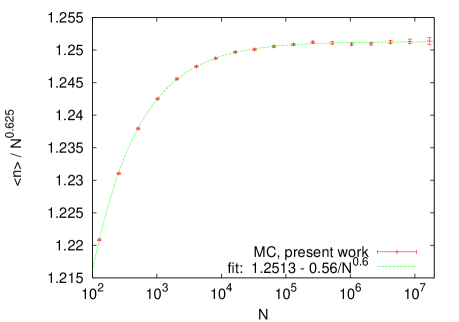
Our results are summarized in Table 1 and in Figs. 1 to 3. Figure 1 shows that our data for $d=2$ are perfectly consistent with $D=5/4$, as expected. It also shows that the corrections to scaling are quantitatively described by a single power with exponent $\Delta=0.6$. There is to our knowledge no theoretical prediction for the latter, although it should be possible to obtain one from conformal invariance.

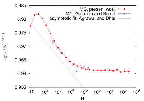
The data for $d=3$ shown in Fig. 2 are much more interesting. The first surprise is that a single power would not be enough to describe the corrections to scaling, due to the lack of convexity of the curve $\langle n\rangle$ versus $\log N$. In view of this we refrain from quoting a value for the leading correction exponent, and we quote rather large errors for the scaling exponent:

$$D=1.6236\pm 0.0004\quad(d=3).$$ (7)

Although this error is equal to the error quoted in Ref. Agrawal , we believe that we can firmly exclude the latter estimate, which is about 13 standard deviations away from our estimate. In order to illustrate the contradiction between our two estimates, we plotted in Fig. 2 also the asymptotic behavior based on the estimate of Ref. Agrawal .

This estimate was obtained not by measuring $\langle n\rangle$ versus $N$, but by measuring the loop size distribution. To obtain $D$ from this, the authors of Agrawal had to make a parameterized scaling ansatz for it. This ansatz had also to take into account that the loop size distribution has a cut off for finite $N$. It might be that either the ansatz was not general enough to take into account the finite-size corrections seen in Fig. 2, or that the cut off was parameterized wrongly. In contrast, the authors of Ref. Bursill used $\langle n\rangle$ versus $N$, as we do. They also cited their raw data, and as seen from Fig. 2 they are in perfect agreement with our simulations.

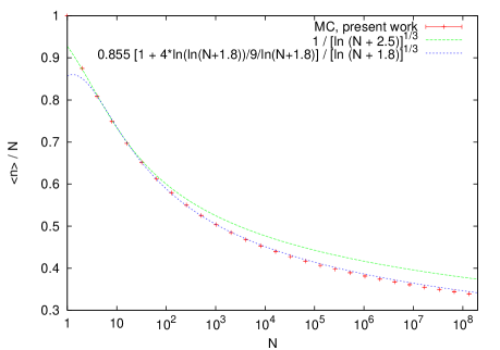
Finally, our data for $d=4$ are shown in Fig. 3. Without logarithmic corrections we would have $\langle n\rangle/N=const$. Equations (4) and (5) contain in principle also arbitrary integration constants and, in addition, the results of higher order corrections. This can be taken into account by replacing $N$ in a numerical analysis by $N/N_{0}$ or, alternatively, by $N+N_{0}$. A priori neither seems preferred. For both choices the constant $N_{0}$ is unknown and can take different values in Eqs. (4) and (5). We found that using the second (additive) choice gave better fits, and will use it in the following. We determined $N_{0}$ somewhat arbitrarily such that the MC data fitted the analytic expressions for $4\leq N\leq 16$. In both cases (leading log and two loops) this gave $N_{0}$ roughly of order 1 (more precisely, 2.5 and 1.8). The main conclusion from Fig. 3 is that our MC data agree qualitatively with the leading log predictions, but not perfectly. This difference is nearly completely eliminated when the two-loop correction is included. There remains a small residual difference, but we can definitely say that including the two-loop correction gives a big improvement and suggests that the FRG is basically correct.

IV Conclusion

Our simulations indicate clearly that the FRG analysis of Ref. Fedorenko is basically correct in four dimensions, where its predictions should be most reliable. It is less successful in $d=3$, where it gives a too big change over the one-loop result. The latter conclusion depends on our new estimate for the fractal LERW dimension in $d=3$, which is about 13 (new and old) standard deviations away from the best previous estimate. Finally, we verify the known value of the fractal dimension in $d=2$ with higher precision than previous Monte Carlo analyses, and we present estimates for the correction to scaling exponent in $d=2$. It should be possible to calculate the latter analytically from conformal invariance.

Acknowledgments: I am indebted to Prof. Andrei Fedorenko for bringing this problem to my attention. I also want to thank him and Profs. Pierre Le Doussal, Kay Wiese and Deepak Dhar for very helpful correspondences.

References

- (1) S.N. Majumdar, Phys. Rev. Lett. 68, 2329 (1992).
- (2) B. Duplantier, Physica A 191, 516 (1992).
- (3) O. Schramm, Israel J. Math. 118, 221 (2000).
- (4) G.F. Lawler, Duke Math. J. 47, 655 (1980).
- (5) G.F. Lawler, Special issue of J. Fourier Anal. Appl. 347 (1995).
- (6) A.A. Fedorenko, P. Le Doussal, and K.J. Wiese, J. Stat. Phys. 133, 805 (2008).
- (7) H. Agrawal and D. Dhar, Phys. Rev. E 63, 056115 (2001).
- (8) A.J. Guttmann and R.J. Bursill, J. Stat. Phys. 59, 1 (1990).
- (9) H.-P. Hsu and P. Grassberger, J. Stat. Mech. P01007 (2005).
- (10) P. Grassberger, Phys. Rev. E 67, 036101 (2003).
- (11) P. Grassberger, Phys. Rev. E to be published (2009).
- (12) R.M. Ziff, Computers in Physics 12, 385 (1998).