Time$-$metric equivalence and dimension change under time reparameterizations

Abstract

We study the behavior of dynamical systems under time reparameterizations, which is important not only to characterize chaos in relativistic systems but also to probe the invariance of dynamical quantities. We first show that time transformations are locally equivalent to metric transformations, a result that leads to a transformation rule for all Lyapunov exponents on arbitrary Riemannian phase spaces. We then show that time transformations preserve the spectrum of generalized dimensions $D_{q}$ except for the information dimension $D_{1}$, which, interestingly, transforms in a nontrivial way despite previous assertions of invariance. The discontinuous behavior at $q=1$ can be used to constrain and extend the formulation of the Kaplan-Yorke conjecture.

Recent studies of chaos in general relativity and cosmology highlighted the importance of the time parameterization as an extra dimension in the characterization of chaotic dynamics Mot:03 . Ever since Lyapunov exponents and other dynamical quantities were found to depend on the choice of the time parameter FraMat:88 , much effort has been directed towards an invariant characterization of chaos that would avoid the difficulties imposed by this dependence Hobill:94 ; Gurzadyan:00 ; Cornish:97 ; Cipriani:98 ; Mot:2001 . However, at the most fundamental level, one could instead seek to explore the freedom introduced by time transformations in order to investigate the dependence of the dynamical quantities on the geometrical versus temporal properties of the orbits, which is an important and often elusive open problem. This problem can be traced to the question of how dynamical quantities change under time transformations.

In this Rapid Communication, we consider the dynamical effect of spatially inhomogeneous time transformations (i.e., time reparameterizations that depend on the phase-space coordinates). From the perspective of the rate of separation between nearby trajectories, we show that the time reparameterizations can be identified with local transformations of the phase-space metric. This implies that all Lyapunov exponents of a given orbit are scaled by a common factor and the resulting Lyapunov dimension is invariant under time transformations. We show, however, that the information dimension is generally not invariant in non-ergodic systems, illustrating that the identity between the information dimension and the Lyapunov dimension of average Lyapunov exponents generally does not hold in such systems; noticeably, the other generalized dimensions remain invariant in spite of their dependence on the invariant measure, which does change.

Numerous physical systems can be described as smooth dynamical systems of the form

$$\frac{d\bm{x}}{dt}=\bm{f}(\bm{x})$$ (1)

defined on a smooth Riemannian manifold $M$ of certain metric $g$, which represents the phase space of the system. We focus on this general class of systems and consider time reparameterizations of the form

$$d\tau=r(\bm{x})dt,$$ (2)

where $r$ is a smooth and strictly positive integrable function. We also assume that $r$ and $r^{-1}$ are bounded away from zero on the asymptotic sets of the system. These conditions assure that $\tau(\bm{x}_{o},t)=\int_{0}^{t}r(\bm{x}(t^{\prime}))dt^{\prime}$, where $\bm{x}_{o}\equiv\bm{x}(0)$, is a well-defined time parameter. In the case of Friedmann-Robertson-Walker cosmological models, for instance, the proper time $T$ and the conformal time $\eta$ are related through the relation $dT=ad\eta$, where the dynamical variable $a$ is positive away from cosmological singularities PRD2002 . But the reparameterization (2) is not limited to relativistic systems, in that it can represent any change of independent variable; parameter $\tau$ could be, for example, a monotonically increasing angular coordinate.

We first note CorFomSin:82 that the time reparameterization changes an invariant probability measure from $\mu$ to $\mu_{r}$ according to

$$d\mu_{r}=\frac{r}{\int_{M}rd\mu}d\mu\,.$$ (3)

This change applies, in particular, to natural probability measures, despite the fact that the orbits remain invariant and ergodicity is preserved by time reparameterizations CorFomSin:82 . Physically, this reflects the fact that the transformed system evolves at different speeds and hence with different residence times along the orbits result0 .

Next we note that the Lyapunov exponents,

$$\lambda(\bm{x}_{o},\bm{v}_{o})=\limsup_{t\to\infty}\frac{1}{t}\log\lVert\bm{v}(\bm{x}_{o},t)\rVert,$$ (4)

may change as the time is reparameterized FraMat:88 ; Mot:03 . Here $\bm{v}(\bm{x}_{o},t)$ is the solution of the variational equation of system (1) for an initial condition $\bm{x}_{o}$ and an initial vector $\bm{v}_{o}$ modeling the distance between nearby trajectories, and $\lVert\cdot\rVert$ is the norm induced by the Riemannian metric. The time transformation generally changes the length and direction of the vectors $\bm{v}(\bm{x}_{o},t)$ for $t>0$, which are then denoted by $\bm{v}_{r}(\bm{x}_{o},\tau(\bm{x}_{o},t))$. However, we now show that an equivalent change can be induced by a transformation of the metric.

Specifically, we construct a Riemannian metric $\widetilde{g}$ on $M$ such that for any two vectors $\bm{v}_{o}$ and $\bm{w}_{o}$ in the tangent space $T_{\bm{x}_{o}}M$ of $M$ at $\bm{x}_{o}$ we have

$$\left\langle\bm{v}(\bm{x}_{o},t),\bm{w}(\bm{x}_{o},t)\right\rangle_{\widetilde{g}}=\left\langle\bm{v}_{r}(\bm{x}_{o},\tau(\bm{x}_{o},t)),\bm{w}_{r}(\bm{x}_{o},\tau(\bm{x}_{o},t))\right\rangle_{g}$$ (5)

for every $t$ in some interval $I$ around zero. Here $\bm{v}$ and $\bm{w}$ ($\bm{v}_{r}$ and $\bm{w}_{r}$) correspond to the solutions of the variational equation before (after) the time reparameterization, and $\langle\cdot,\cdot\rangle$ stands for the scalar product induced by the metric. We say that $\widetilde{g}$ and $g$ satisfying (5) are locally related by the time reparameterization $r$ at $\bm{x}_{o}$.

To proceed we consider $N$= $\dim M$ linearly independent vectors $\bm{v}_{j}\in T_{\bm{x}_{o}}M$, $\lVert\bm{v}_{j}\rVert=1$, and denote by $\bm{y}_{j}(t)\equiv\bm{y}(\bm{x}_{o},\bm{v}_{j},t)$ the solution of the variational equation of (1) with $\bm{y}_{j}(0)=\bm{v}_{j}$. With respect to a local representation (and using the summation convention), the variational equation reads

$$\frac{d{y_{j}}^{k}}{dt}=\frac{\partial f^{k}}{\partial x^{i}}{y_{j}}^{i},\;\;k=1,\ldots,N,$$ (6)

and does not depend on the metric. The same argument applies to the solutions $\bm{z}_{j}(t)\equiv\bm{z}(\bm{x}_{o},\bm{v}_{j},\tau(\bm{x}_{o},t))$ of the variational equation after the time transformation,

$$\frac{d{z_{j}}^{k}}{d\tau}=\frac{\partial f^{k}/r}{\partial x^{i}}{z_{j}}^{i},\;\;k=1,\ldots,N,$$ (7)

with $\bm{z}_{j}(0)=\bm{v}_{j}$.

On account of this, condition (5) can be restated as

$$\langle\bm{y}_{i}(t),\bm{y}_{j}(t)\rangle_{\widetilde{g}}=\langle\bm{z}_{i}(t),\bm{z}_{j}(t)\rangle_{g}$$ (8)

for every $i$, $j=1,\ldots,N$ and every $t\in I$. Representing the metric tensor $g$ locally by $G(\bm{x}_{o},t)\equiv\left(g_{ij}(\bm{x}(t))\right)$, Eqs. (8) determine the choice of a family of matrices $G(\bm{x}_{o},t)$ along the trajectory $\bm{x}(t)$. The corresponding system of $N^{2}$ equations can be written in matrix form as

$${Y_{t}}^{\dagger}\widetilde{G}(\bm{x}_{o},t)Y_{t}={Z_{t}}^{\dagger}G(\bm{x}_{o},t)Z_{t},$$ (9)

where ^† denotes the matrix transpose, $\widetilde{G}\equiv\left(\widetilde{g}_{ij}\right)$ denotes the local representation of the metric tensor $\widetilde{g}$, and where $Y_{t}\equiv(\bm{y}_{1}(t),\bm{y}_{2}(t),\ldots,\bm{y}_{N}(t))$ and $Z_{t}\equiv(\bm{z}_{1}(t),\bm{z}_{2}(t),\ldots,\bm{z}_{N}(t))$ are $N\times N$-matrices having the vectors ${\bm{y}}_{j}(t)$ and $\bm{z}_{j}(t)$ as columns. The matrix $Y(t)$ is invertible since $\bm{v}_{1},\ldots,\bm{v}_{N}$ are linearly independent and the linear map $\bm{v}_{o}\rightarrow\bm{v}(\bm{x}_{o},t)$ is invertible. The latter follows from the fact that the flow map $\bm{x}_{o}\rightarrow\bm{x}(t)$ is a diffeomorphism on $M$. Therefore, (9) leads to

$$\widetilde{G}(\bm{x}_{o},t)=(Z_{t}{Y_{t}}^{-1})^{\dagger}G(\bm{x}_{o},t)Z_{t}{Y_{t}}^{-1},$$ (10)

which is the locally related metric that we sought to construct.

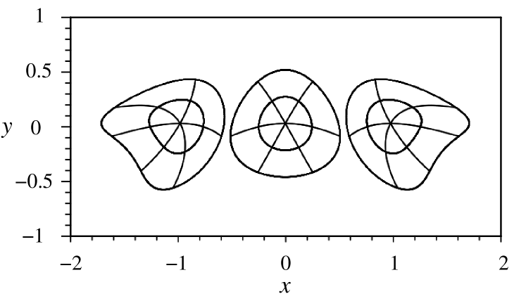
Figure 1: Time-metric equivalence. Geodesic coordinates of metric (11) for three different initial points and contour lines at distances $1/4$ and $1/2$ from these points. In this illustration, all geodesic lines have length 1/2 with respect to the new metric.

A simple example is illustrated in Fig. 1, in which we time transform the linear flow $dx/dt=1$, $dy/dt=0$ with $r(x,y)=e^{-y}$. Given $x(0)=0$ and arbitrary $y(0)$, the metric $\widetilde{g}$ that is locally related to the 2D Euclidean metric is given by the matrix

$$\left(\widetilde{g}_{ij}\right)=\left(\begin{matrix}1&x\\ x&1+x^{2}\end{matrix}\right).$$ (11)

In the figure we show local geodesic coordinates of the new metric, that is, given an initial point we draw the outgoing geodesics of fixed lengths with respect to $\widetilde{g}$. Note that even this simple system exhibits interesting properties due to the shear introduced by the time reparameterization. A few observations are in order.

First, the metric $\widetilde{g}$ defined by (10) does not depend on the initial choice of vectors $\bm{v}_{j}$, $j=1,\ldots,N$. Because the variational equations are linear, we can write $Y_{t}=\Phi(\bm{x}_{o},t)V_{0}$ and $Z_{t}=\Phi_{r}(\bm{x}_{o},\tau(\bm{x}_{o},t))V_{0}$, where $V_{0}=(\bm{v}_{1},\bm{v}_{2},\ldots,\bm{v}_{N})$ is the $N\times N$-matrix having the vectors $\bm{v}_{j}$ as columns and where $\Phi$ and $\Phi_{r}$ are the local representations of the evolution matrices. This leads to $\widetilde{G}(\bm{x}_{o},t)=W(\bm{x}_{o},t)^{\dagger}G(\bm{x}_{o},t)W(\bm{x}_{o},t)$, where $W(\bm{x}_{o},t)\equiv\Phi_{r}(\bm{x}_{o},\tau(\bm{x}_{o},t))\Phi^{-1}(\bm{x}_{o},t)$. Second, the metric $\widetilde{g}$ depends smoothly on the initial conditions and can be extended in a neighborhood of $\bm{x}_{o}$; a smooth extension can be generated for every given smooth surface of initial points passing through $\bm{x}_{o}$ transversely to the flow. Third, the dependence of the metric $\widetilde{g}$ on the time $t$ indicates that, in general, the metric is single-valued only on some finite time interval along the trajectories. For example, the interval $I$ is generally limited by $t_{0}$ if $\bm{x}_{o}$ is a periodic point of period $t_{0}$ (with respect to the time $t$) and the function $r$ is such that $\Phi(\bm{x}_{o},t_{0})\neq\Phi_{r}(\bm{x}_{o},\tau(\bm{x}_{o},t_{0}))$. The interval $I$ is similarly constrained by the recurrence of orbits to the neighborhood in which the metric is extended local_global . Furthermore, the time dependence of the metric can be eliminated in favor of a dependence on $\bm{x}_{o}$ and $\bm{x}$ only. Therefore, our result establishes a local equivalence between time and metric transformations on $M$.

A neat implication of this time-metric equivalence is that, under the time reparameterization (2), the Lyapunov exponent in Eq. (4) changes exclusively due to the transformation of the factor $1/t$. The contribution due to the logarithmic factor remains unchanged because the norms induced by the metrics $g$ and $\widetilde{g}$ are logarithmically equivalent along each orbit local_global ; that is, for each ${\bm{x}_{o}}$ and ${\bm{v}_{o}}$ there is a sub-exponential function $C=C(t)$ such that $||\bm{v}(\bm{x}_{o},t)||_{\widetilde{g}}\equiv||W(\bm{x}_{o},t)\bm{v}(\bm{x}_{o},t)||_{g}=C(t)||\bm{v}(\bm{x}_{o},t)||_{g}$ longpaper . Therefore, the Lyapunov exponents transform as $\lambda_{r}(\bm{x}_{o},\bm{v}_{o})=\lambda(\bm{x}_{o},\bm{v}_{o})/\Lambda(\bm{x}_{o})$, where $\Lambda(\bm{x}_{o})=\lim_{t\rightarrow\infty}\tau(\bm{x}_{o},t)/t$. This extends the result previously derived in Ref. Mot:03 for Euclidean phase spaces to the more general case of Riemannian manifolds.

We now turn to the transformations of fractal dimensions, which cannot be accounted for by metric changes. The box-counting dimension $D_{0}$ is purely geometrical and hence does not change under time reparameterization. The generalized dimensions $D_{q}$, however, can in principle change for $q>0$ given that they depend on the measure and the measure is transformed according to (3). To analyze this dependence, we consider a positive-measure set of interest $S$ (typically an attractor) and define the spectrum of dimensions on $S$ as

$$D_{q}(\mu) = \frac{1}{q-1}\limsup_{\varepsilon\to 0}\frac{1}{\log\varepsilon}\log\sum_{k=1}^{N(\varepsilon)}\mu(B_{k})^{q},\;q\geq 0,q\neq 1,$$ (12)

$$D_{1}(\mu) = \limsup_{\varepsilon\to 0}\frac{1}{\log\varepsilon}\sum_{k=1}^{N(\varepsilon)}\mu(B_{k})\log\mu(B_{k}),$$ (13)

where the sum is taken over the $N(\varepsilon)$ nonzero measure boxes $B_{k}$ of edge length $\varepsilon$ necessary to cover the set grass1983 ; hents1983 ; comment . This spectrum includes as special cases the information dimension ($q=1$) and the correlation dimension ($q=2$). For consistency, the measure is always normalized to 1 on $S$ (with $M$ replaced by $S$ in Eq. (3)). The dimensions $D_{q}$ are known not to depend on smooth transformations of the phase space. We now consider their behavior under time transformations.

The first surprise is that, contrary to what intuition may suggest, the dimensions defined by Eq. (12) are invariant with respect to time transformations not only for $q=0$ but also for all $q\neq 1$. This follows from the fact that $\mu$ and $\mu_{r}$ in Eq. (3) are absolutely continuous with respect to each other, i.e., both measures define the same sets of nonzero measure, and that $r$ and $r^{-1}$ are bounded away from zero on these sets. Then there exist positive constants $c_{1}$, $c_{2}$ such that $c_{1}\mu(B_{k})\leq\mu_{r}(B_{k})\leq c_{2}\mu(B_{k})$ for every $k$ and $\varepsilon>0$. Using this in the definition (12), we obtain

$$D_{q}(\mu_{r})=D_{q}(\mu)\;\;\mbox{for }q\geq 0,q\neq 1,$$ (14)

i.e., the dimensions remain unchanged despite their dependence on the measure, which generally changes.

The second surprise is that the information dimension (13) exhibits a distinctive behavior and may change under the same time reparameterization. To appreciate this, we first notice that Eq. (13) can be written in the continuous form $D_{1}(\mu)=\limsup_{\varepsilon\to 0}\frac{1}{\log\varepsilon}\int_{S}\log\mu(B(\bm{x},\varepsilon))\,d\mu(\bm{x})$, where $B(\bm{x},\varepsilon)$ is an open ball of radius $\varepsilon$ centered at $\bm{x}$. We then use the Fatou lemma to obtain

$$D_{1}(\mu)\leq\int_{S}\limsup_{\varepsilon\to 0}\frac{1}{\log\varepsilon}\log\mu(B(\bm{x},\varepsilon))\,d\mu(\bm{x}),$$ (15)

where the integrand is the pointwise dimension, which we denote by $\overline{\cal D}_{\mu}(x)$. A similar inequality holds for the infimum, in which case the pointwise dimension is denoted by $\underline{\cal D}_{\mu}(\bm{x})$. This leads to

$$\int_{S}\underline{\cal D}_{\mu}(\bm{x})\,d\mu(\bm{x})\leq D_{1}(\mu)\leq\int_{S}\overline{\cal D}_{\mu}(\bm{x})\,d\mu(\bm{x}).$$ (16)

In the remaining part of the paper we limit the discussion to the case $\underline{\cal D}_{\mu}(\bm{x})=\overline{\cal D}_{\mu}(\bm{x})\equiv{\cal D}_{\mu}(\bm{x})$ almost everywhere, a property found in many physical systems and demonstrated for flows with strong hyperbolic behavior hyper . This assures that the equalities hold in (16).

The transformed information dimension is then written as

$$D_{1}(\mu_{r})=\int_{S}\frac{r(\bm{x})}{\int_{S}rd\mu}{\cal D}_{\mu}(\bm{x})d\mu(\bm{x}),$$ (17)

where we have used the measure (3) normalized on $S$ and the invariance of the pointwise dimension. The latter follows from (3) and is stated as ${\cal D}_{\mu_{r}}(\bm{x})={\cal D}_{\mu}(\bm{x})$ for almost every $\bm{x}$. The result in (17) indicates that $D_{1}$ is in general noninvariant when ${\cal D}_{\mu}(\bm{x})$ is not almost everywhere constant.

For example, consider a system with two ergodic components, $S_{A}$ and $S_{B}$, of information dimension $D_{1}(\mu|S_{A})>D_{1}(\mu|S_{B})$. For simplicity, assume that the original measure is evenly split between the two sets, i.e. $\mu(S_{A})=\mu(S_{B})$, and that $\mu(B_{k})$ is the same for all the nonzero measure boxes $B_{k}$ of each set. The information dimension of $S=S_{A}\cup S_{B}$ is $D_{1}(\mu)=\frac{1}{2}[D_{0}(S_{A})+D_{0}(S_{B})]$. Now, imagine a time reparameterization that changes $\mu|S_{1}$ uniformly by a factor $0<\alpha<2$ and $\mu|S_{2}$ uniformly by a factor $\beta=2-\alpha$. The transformed information dimension is $D_{1}(\mu_{r})=\frac{\alpha}{2}D_{0}(S_{A})+\frac{2-\alpha}{2}D_{0}(S_{B})$, which differs from $D_{1}(\mu)$ for any $\alpha\neq 1$ entangled .

In the case of $q\neq 1$, this change in the measure contributes an additive term to $\log\sum_{k}\mu(B_{k})^{q}$ in Eq. (12) that vanishes when divided by $\log\varepsilon$ in the limit of small $\varepsilon$, in agreement with our prediction that the other dimensions $D_{q}$ are all invariant. At first sight the noninvariance for $q=1$ may seem to violate the monotonicity of $D_{q}$, which was previously proved to hold for $0\leq q<1$ and for $q>1$ grass1983 , but this intuition is misleading because $\lim_{q\rightarrow 1-}D_{q}>\lim_{q\rightarrow 1+}D_{q}$ whenever ${\cal D}_{\mu}(\bm{x})$ is not constant and $D_{1}$ is not invariant. In our example, when $q<1$, the contribution $\sum_{k}\mu(B_{k})^{q}$ from the set with the largest box-counting dimension dominates and leads to $D_{q<1}=D_{0}(S_{A})$, just as in the case $q=0$; when $q>1$, the box-counting dimension of the other set dominates, and $D_{q>1}=D_{0}(S_{B})$. The information dimension $D_{1}(\mu_{r})$ is thus a weighted average of the dimensions on both sides of the discontinuity and is in general free to vary between $\lim_{q\rightarrow 1-}D_{q}$ and $\lim_{q\rightarrow 1+}D_{q}$ under time reparameterizations, as shown in Fig. 2.

Figure 2: Dimension change. The gap between the generalized dimensions on the left and right sides of $q=1$ is invariant and determines the interval of possible changes for $D_{1}$ under time transformations. The Lyapunov dimension $D_{L}$ remains invariant, whereas the Lyapunov dimension $\tilde{D}_{L}$ transforms as $D_{1}$

.

The information dimension is guaranteed to be invariant only in special cases. The most important such case is when $\mu$ (and hence $\mu_{r}$) is ergodic in $S$. Since the flow map $\bm{x}_{o}\rightarrow\bm{x}(t)$ is a diffeomorphism and the measure is invariant under this map, one can verify that ${\cal D}_{\mu}(\bm{x}_{o})={\cal D}_{\mu}(\bm{x}(t))$. Then, if $\mu$ is ergodic, ${\cal D}_{\mu}(\bm{x})$ is constant for almost every $\bm{x}$, and hence $D_{1}(\mu_{r})=D_{1}(\mu)$. The general condition for $D_{1}$ to be invariant with respect to any time transformation is that ${\cal D}_{\mu}(\bm{x})$ is constant almost everywhere.

It is of interest to analyze the meaning of the noninvariance of $D_{1}$ for the Kaplan-Yorke conjecture ld1 ; ld2 and its generalizations, which state that the information dimension typically equals the Lyapunov dimension. Let the average Lyapunov exponents be $\lambda_{i}=\int\lambda_{i}(\bm{x})d\mu(\bm{x})$, where $\lambda_{1}(\bm{x})\geq\lambda_{2}(\bm{x})\geq\dots\geq\lambda_{N}(\bm{x})$ corresponds to the ordered set of Lyapunov exponents (4) at $\bm{x}$, and assume that this definition is applied to measures that are not necessarily proved to be ergodic. Based on the definition operationally used in numerical experiments, the Lyapunov dimension can be defined as

$$D_{L}(\mu)=K+\frac{1}{|\lambda_{K+1}|}\sum_{j=1}^{K}\lambda_{i},$$ (18)

where $K$ is the largest integer such that $\sum_{j=1}^{K}\lambda_{i}\geq 0$, under the condition that the r.h.s. terms in (18) are well defined. It follows that $D_{L}(\mu)$ remains invariant under time reparameterizations, thus violating the equality $D_{L}=D_{1}$ when $D_{1}$ changes. In the example considered above, the Lyapunov dimension of $S=S_{A}\cup S_{B}$ is intermediate between the Lyapunov dimensions of $S_{A}$ and $S_{B}$, indicating that $D_{L}$ equals $D_{1}$ for at most one value of $\alpha$. The conjecture can be re-established, however, for the Lyapunov dimension defined as

$$\tilde{D}_{L}(\mu)=\int\{K(\bm{x})+\frac{1}{|\lambda_{K(\bm{x})+1}(\bm{x})|}\sum_{j=1}^{K(\bm{x})}\lambda_{i}(\bm{x})\}d\mu(\bm{x}),$$ (19)

where $K$ is defined as above but now at each point $\bm{x}$ (with the convention that the integrand is zero for $\lambda_{1}(\bm{x})<0$ and $N$ for $\lambda_{N}(\bm{x})>0$). It follows from (17) and the Kaplan-Yorke conjecture for typical ergodic sets that the identity $D_{1}=\tilde{D}_{L}$ is expected to hold true for generic systems (see Fig. 2).

The noninvariance of the information dimension, which was previously surmised to be invariant Cornish:97 , is important as it limits the applicability of the identity $D_{L}=D_{1}$ in nonergodic systems and ergodicity is a property often difficult to verify. The invariance of other indicators of chaos established in this paper is relevant to the study of a range of dynamical phenomena, including spatiotemporal chaos, and clarifies longstanding problems in relativistic chaos. It shows, in particular, the observer invariance of the often questioned chaoticity of the mixmaster model for the early universe Hobill:94 , which was first recognized as a chaotic geodesic flow on a Riemannian manifold by Chitre in 1972 in a work that made one of the very first uses of the term “chaos” in dynamics chitre72 .

References

- (1) A. E. Motter, Phys. Rev. Lett. 91, 231101 (2003); A. E. Motter and A. Saa, ibid. 102, 184101 (2009).
- (2) G. Francisco and G. E. A. Matsas, Gen. Relativ. Gravit. 20, 1047 (1988).
- (3) D. Hobill, A. Burd, and A. Coley (Eds.), Deterministic Chaos in General Relativity (Plenum, 1994).
- (4) V. G. Gurzadyan and R. Ruffini (Eds.), The Chaotic Universe (World Scientific, 2000).
- (5) N. J. Cornish and J. J. Levin, Phys. Rev. D 55, 7489 (1997).
- (6) P. Cipriani and M. Di Bari, Phys. Rev. Lett. 81, 5532 (1998).
- (7) A. E. Motter and P. S. Letelier, Phys. Lett. A 285, 127 (2001).
- (8) A. E. Motter and P. S. Letelier, Phys. Rev. D 65, 068502 (2002).
- (9) I. Cornfeld, S. Fomin, and Y. Sinai, Ergodic Theory (Springer, 1982).
- (10) The inverse transformation of (3) is well-defined since the integrability of with respect to assures the integrability of with respect to .
- (11) Along a single orbit, as considered in the transformation of Lyapunov exponents, the metric can always be extended as a single-valued function over the entire orbit; in periodic orbits, it can be extended as a single-valued function over the period of the orbit and as a multi-valued function beyond it.
- (12) This relation follows from the sub-exponential evolution of the angles between the Lyapunov vectors and holds for almost every .
- (13) P. Grassberger, Phys. Lett. A 97, 227 (1983).
- (14) H. G. E. Hentschel and I. Procaccia, Physica D 8, 435 (1983).
- (15) Similar definitions and results can be established for limsup replaced by liminf.
- (16) This class of systems includes all geodesic flows on compact Riemannian manifolds with negative curvature BarRadWol:04 , which play a significant rule, for instance, in the characterization of chaos in mixmaster cosmologies chitre72 ; burd93 .
- (17) L. Barreira, L. Radu, and C. Wolf, Dyn. Syst. 19, 89 (2004).
- (18) D. M. Chitre, Ph.D. Thesis, Univ. of Maryland (1972).
- (19) A. Burd and R. Tavakol, Phys. Rev. D 47, 5336 (1993).
- (20) Similar behavior is found even when the two sets are intermingled. The details will be included in an extended paper.
- (21) J. L. Kaplan and J. A. Yorke, Lect. Notes Math. 730, 204 (1979).
- (22) J. D. Farmer, E. Ott, and J. A. Yorke, Physica D 7, 153 (1983).