Spatial averaging and apparent acceleration in inhomogeneous spaces
Abstract
As an alternative to dark energy that explains the observed acceleration of the universe, it has been suggested that we may be at the center of an inhomogeneous isotropic universe described by a Lemaitre-Tolman-Bondi (LTB) solution of Einstein’s field equations. To test this possibility, it is necessary to solve the null geodesics. In this paper we first give a detailed derivation of a fully analytical set of differential equations for the radial null geodesics as functions of the redshift in LTB models. As an application we use these equaions to show that a positive averaged acceleration obtained in LTB models through spatial averaging can be incompatible with cosmological observations. We provide examples of LTB models with positive which fail to reproduce the observed luminosity distance . Since the apparent cosmic acceleration is obtained from fitting the observed luminosity distance to a FLRW model we conclude that in general a positive in LTB models does not imply a positive .
I Introduction
High redshift luminosity distance measurements Perlmutter:1998np ; Riess:1998cb ; Tonry:2003zg ; Knop:2003iy ; Barris:2003dq ; Riess:2004nr and the WMAP measurement WMAP2003 ; Spergel:2006hy of cosmic microwave background (CMB) interpreted in the context of standard FLRW cosmological models have strongly disfavored a matter dominated universe, and strongly supported a dominant dark energy component, giving rise to a positive cosmological acceleration, which we will denote by (not to be confused with the scale factor ). As an alternative to dark energy, it has been proposed Nambu:2005zn ; Kai:2006ws that we may be at the center of an inhomogeneous isotropic universe described by a Lemaitre-Tolman-Bondi (LTB) solution of Einstein’s field equations, where spatial averaging over one expanding and one contracting region is producing a positive averaged acceleration . Another more general approach is to directly map luminosity distance as a function of redshift to LTB models Celerier:1999hp ; Iguchi:2001sq , and more recently different groups Chung:2006xh ; Yoo:2008su have shown that an inversion method can be applied successfully to reproduce the observed . The main point is that the luminosity distance is in general sensitive to the geometry of the space through which photons are propagating along null geodesics, and therefore arranging appropriately the geometry of a given cosmological model it is possible to reproduce a given .
The averaged acceleration on the other side is not directly related to , since the latter is obtained by integrating the position dependent cosmological redshift along the null geodesics, while is the result of spatial averaging, and has no relation to the causal structure of the underlying space. It was shown Romano:2006yc that this crucial difference can make unobservable to a central observer when the scale of the spatial averaging is greater than its event horizon.
In this paper we will further investigate the relation between LTB models with positive averaged acceleration and cosmological observations, showing that in general they can be incompatible. Different authors have studied acceleration in LTB spaces Hirata:2005ei ; Vanderveld:2006rb using different definitions, showing that the deceleration parameter deduced from the luminosity distance observation cannot be negative if the origin of an LTB model is regular and smooth. But they did not focus on models with spatially averaged acceleration as we do.
It should also be mentioned the work by Bolejko:2008yj , where some models with positive averaged acceleration are shown to be unrealistic. On the other hand, what we show is that for models with positive averaged acceleration, apparent defined from the luminosity distance is not negative, which in principle could have become negative, independent of whether such models are unrealistic or not.
II Lemaitre-Tolman-Bondi (LTB) Solution
Lemaitre-Tolman-Bondi solution can be written as Lemaitre:1933qe ; Tolman:1934za ; Bondi:1947av
| (1) |
where is a function of the time coordinate and the radial coordinate , , is an arbitrary function of , and .
Einstein’s equations give
| (2) | |||||
| (3) |
with being an arbitrary function of and the dot denoting the partial derivative with respect to , . The solution of Eq. (2) can be expressed parametrically in terms of a time variable as
| (4) | |||||
| (5) |
where has been introduced to make clear the distinction between the two functions and which are trivially related by
| (6) |
and is another arbitrary function of , called the bang function, which corresponds to the fact that big-bang/crunches can happen at different times. This inhomogeneity of the location of the singularities is one of the origins of the possible causal separation Romano:2006yc between the central observer and the spatially averaged region for models with positive .
We introduce the variables
| (7) |
so that Eq. (1) and the Einstein equations (2) and (3) are written in a form similar to those for FLRW models,
| (8) |
| (9) | |||||
| (10) |
The solution of Eqs. (4) and (5) can now be written as
| (11) | |||||
| (12) |
where .
In the rest of paper we will use this last set of equations and drop the tilde to make the notation simpler. Furthermore, without loss of generality, we may set the function to be a constant, .
III Geodesic equations
The luminosity distance for a central observer in a LTB space as a function of the redshift is expressed as
| (13) |
where or is the solution of the radial geodesic equation as a function of the redshift. The past-directed radial null geodesic is given by
| (14) |
where is the time coordinate along the null radial geodesic as a function of the the coordinate . Applying the definition of red-shift it is possible to obtain Celerier:1999hp :
| (15) | |||||
| (16) |
or in terms of the function
| (18) | |||||
| (19) |
In order to solve the above differential equations we need which can only be obtained numerically by integrating the Einstein’s equations, while the analytical solution is expressed in terms of . For this reason it is convenient to re-write the above equations in terms of the coordinates . From the implicit solution, we can write
| (20) | |||
| (21) |
where is the coordinate along the null radial geodesic as a function of the the coordinate . In order to perform the change of variables from to we need to use the fact that the derivation of the implicit solution is based on the use of the conformal time variable , which by construction satisfies the relation
| (22) |
from which, after a careful treatment of the partial derivatives, we can derive the following relations:
| (23) | |||||
| (24) | |||||
| (25) | |||||
| (26) |
We can now write :
| (27) |
from which using the geodesic equations (18,19) we get:
| (28) |
We can then express and in terms of the analytical solution using:
| (29) | |||||
| (30) | |||||
| (31) | |||||
| (32) | |||||
| (33) | |||||
Finally we get:
| (34) | |||||
| (35) |
where is the value of the variable along the null geodesic.
It is important to observe that the functions have an explicit analytical form which can be obtained from and using the relations above. In this way the coefficients of equations (34) and (35) are fully analytical, which is a significant improvement over previous approaches which required a numerical integration of the Einstein’s equations. This version of the geodesics equations takes full advantage of the existence of the analytical solution and is suitable for both numerical and analytical applications such as low red-shift expansions.
IV Averaged acceleration
Following the standard averaging procedure Buchert:1999mc ; Palle:2002zf ; Nambu:2005zn we define the volume for a spherical domain, , as
| (36) |
and the length associated with the domain as
| (37) |
Then the deceleration parameter and the averaged acceleration (not to be confused with the scale factor ) are defined as
| (38) | |||||
| (39) |
As models that give a positive averaged acceleration, we consider those studied in Chuang:2005yi . They are characterized by the functions and given by
| (40) | |||||
| (41) |
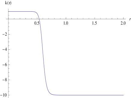
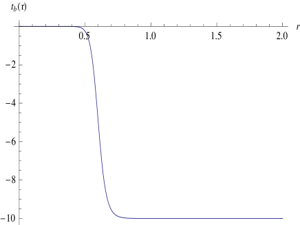
Note that they fix the length scale by setting . After exploring the 9 parameters space they give three examples of LTB solutions with positive as shown in Table I.
| 1 | ||||||||||
| 2 | ||||||||||
| 3 |
| 1 | ||||
| 2 | ||||
| 3 |
Defining as the time in the first column of Table I, i.e. the time at which , with being the value in the last column of the same table, we solved the null geodesics equations (34) and (35) imposing the following initial conditions.
| (42) | |||||
| (43) |
where is obtained by solving numerically for , Eq. (12),
| (44) |
For the second and third model of Table I which we will study we obtain, respectively,
| (45) | |||||
| (46) |
Eq. (42) is the natural way to map these models into luminosity distance observations for a central observer which should receive the light rays at the time at which the averaged acceleration is positive.
V Comparing LTB to observations
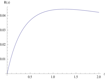
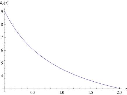
An important model independent quantity is the expansion history, , whose value can be reconstructed from observations of the luminosity distance, , via a single differentiation st98 ; HT99 ; chiba99 ; saini00 ; chiba00
| (47) |


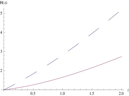
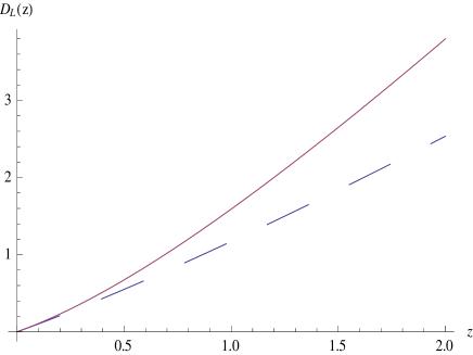
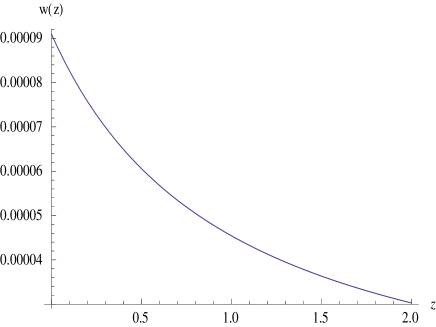
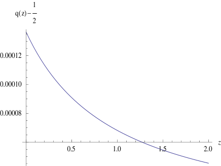
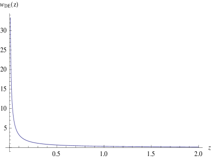
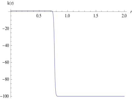
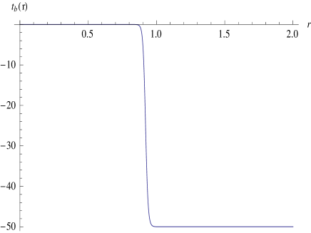

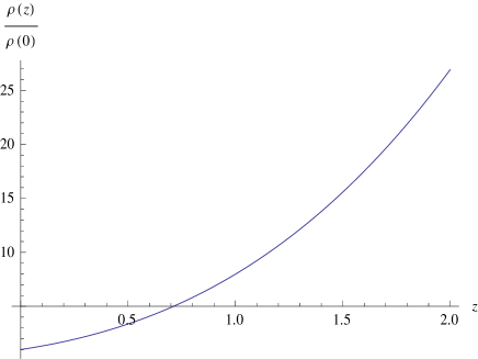
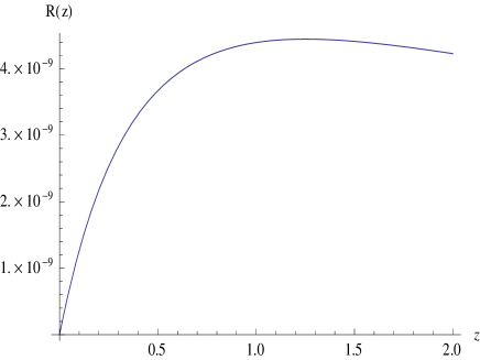
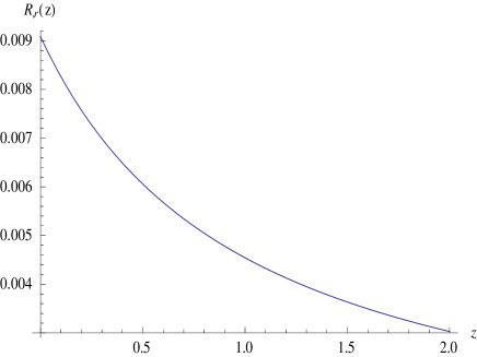
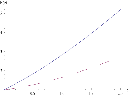
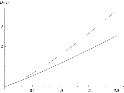
Note that this assumes the universe is not only homogeneous and isotropic but also spatially flat. The equation of state, , of DE is more cumbersome to reconstruct since it involves second derivatives of and is therefore a noisier quantity than . An additional source of uncertainty relating to is caused by the fact that the value of the matter density, enters into the determination of explicitly, through the expression
| (48) |
In our case we can first calculate according to the LTB solutions geodesics equation we derived in the previous section, and then use it to construct and according to Eqs. (48) and (47).
We compare and to the observed and using the standard best fitted FLRW cosmological model,
| (49) | |||||
| (50) |
It should be noted that the parameters given in Table I require to fix the units, and we do that by imposing
| (51) |
In this way we eliminate any ambiguity in the choice of units in order to be able to compare the observed and .
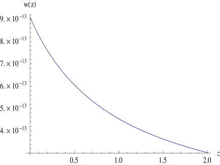
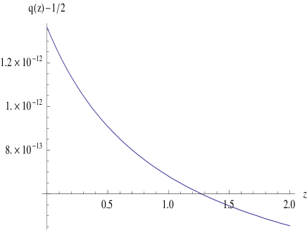
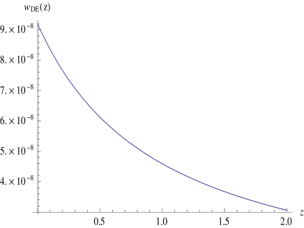
For both the second and third models in Table I, and are not reproducing correctly observational data both from the quantitative and qualitative points of view. The effective is small and positive and the effective is not for both the second and third models. On the contrary, for the redshift range of , for the second model, while for the third model.
As it can be seen from the plots, is approximatively constant in the observationally interesting redshift range, but given the parameters of these models matter is dominating at the time , since as shown above , which explains why is so small and .
These examples show how a positive does not imply a luminosity distance compatible with observations, and gives a reverse example of the results obtained in Enqvist:2006cg , where they obtained a LTB model which fits the observed luminosity distance, consistent with a positive , but without positive averaged acceleration . Our results do not rule out LTB models as alternatives to dark energy since the inversion method Chung:2006xh ; Yoo:2008su allows us to obtain the observed luminosity distance without any averaging, and some concrete examples derived independently have already been proposed Alnes:2006uk ; Alnes:2005rw ; Enqvist:2006cg ; Alexander:2007xx ; Biswas:2007gi ; Tomita:2000jj .
VI Discussion
We have derived a set of differential equations for the radial null geodesics in LTB space-time which takes full advantage of the anaytical solution. We have then used them to compute the luminosity distance for models which have positive spatial acceleration and extended our analysis to other observables such as and , explicitly showing that they are not compatible with the best fit model . Our conclusions do not rule out LTB models as alternatives to dark energy, but provide further evidence that physical quantities obtained via spatial averaging are not relevant to explain observational data.
In the future it will be interesting to find general analytical results in support of our conclusions and to use the equations we derived to provide a new method to solve the inversion problem of mapping the observed luminosity distance to LTB models.
Acknowledgements.
We thank A. Starobinsky and A. Notari for useful comments and discussions. A. E. Romano was supported by JSPS. This work was also supported in part by JSPS Grant-in-Aid for Scientific Research (A) No. 21244033, and by JSPS Grant-in-Aid for Creative Scientific Research No. 19GS0219, and by Monbukagaku-sho Grant-in-Aid for the global COE program, ”The Next Generation of Physics, Spun from Universality and Emergence”.References
- (1) A. G. Riess et al. [Supernova Search Team Collaboration], Astron. J. 116, 1009 (1998) [arXiv:astro-ph/9805201].
- (2) S. Perlmutter et al. [Supernova Cosmology Project Collaboration], Astrophys. J. 517, 565 (1999) [arXiv:astro-ph/9812133].
- (3) J. L. Tonry et al. [Supernova Search Team Collaboration], Astrophys. J. 594, 1 (2003) [arXiv:astro-ph/0305008].
- (4) R. A. Knop et al. [The Supernova Cosmology Project Collaboration], Astrophys. J. 598, 102 (2003) [arXiv:astro-ph/0309368].
- (5) B. J. Barris et al., Astrophys. J. 602, 571 (2004) [arXiv:astro-ph/0310843].
- (6) A. G. Riess et al. [Supernova Search Team Collaboration], Astrophys. J. 607, 665 (2004) [arXiv:astro-ph/0402512].
-
(7)
C. L. Bennett et al.,
Astrophys. J. Suppl. 148, 1 (2003)
[arXiv:astro-ph/0302207];
D. N. Spergel et al. [WMAP Collaboration], Astrophys. J. Suppl. 148, 175 (2003) [arXiv:astro-ph/0302209]. - (8) D. N. Spergel et al., arXiv:astro-ph/0603449.
- (9) Y. Nambu and M. Tanimoto, arXiv:gr-qc/0507057.
- (10) T. Kai, H. Kozaki, K. i. nakao, Y. Nambu and C. M. Yoo, Prog. Theor. Phys. 117, 229 (2007) [arXiv:gr-qc/0605120].
- (11) M. N. Celerier, Astron. Astrophys. 353, 63 (2000) [arXiv:astro-ph/9907206].
- (12) H. Iguchi, T. Nakamura and K. i. Nakao, Prog. Theor. Phys. 108, 809 (2002) [arXiv:astro-ph/0112419].
- (13) D. J. H. Chung and A. E. Romano, Phys. Rev. D 74, 103507 (2006) [arXiv:astro-ph/0608403].
- (14) C. M. Yoo, T. Kai and K. i. Nakao, Prog. Theor. Phys. 120, 937 (2008) [arXiv:0807.0932 [astro-ph]].
- (15) A. E. Romano, Phys. Rev. D 75, 043509 (2007) [arXiv:astro-ph/0612002].
- (16) C. M. Hirata and U. Seljak, Phys. Rev. D 72, 083501 (2005) [arXiv:astro-ph/0503582].
- (17) R. A. Vanderveld, E. E. Flanagan and I. Wasserman, Phys. Rev. D 74, 023506 (2006) [arXiv:astro-ph/0602476].
- (18) K. Bolejko and L. Andersson, JCAP 0810, 003 (2008) [arXiv:0807.3577 [astro-ph]].
- (19) G. Lemaitre, Annales Soc. Sci. Brux. Ser. I Sci. Math. Astron. Phys. A 53, 51 (1933).
- (20) R. C. Tolman, Proc. Nat. Acad. Sci. 20, 169 (1934).
- (21) H. Bondi, Mon. Not. Roy. Astron. Soc. 107, 410 (1947).
- (22) D. Palle, Nuovo Cim. 117B, 687 (2002) [arXiv:astro-ph/0205462].
- (23) T. Buchert, Gen. Rel. Grav. 9, 306 (2000) [arXiv:gr-qc/0001056].
- (24) C. H. Chuang, J. A. Gu and W. Y. Hwang, arXiv:astro-ph/0512651.
- (25) A. A. Starobinsky, JETP Lett. 68, 757 (1998) [Pisma Zh. Eksp. Teor. Fiz. 68, 721 (1998)] [arXiv:astro-ph/9810431].
- (26) D. Huterer and M. S. Turner, Phys. Rev. D 60, 081301 (1999) [arXiv:astro-ph/9808133].
- (27) T. Nakamura and T. Chiba, Mon. Not. Roy. Astron. Soc. 306, 696 (1999) [arXiv:astro-ph/9810447].
- (28) T. D. Saini, S. Raychaudhury, V. Sahni and A. A. Starobinsky, Phys. Rev. Lett. 85, 1162 (2000) [arXiv:astro-ph/9910231].
- (29) T. Chiba and T. Nakamura, Phys. Rev. D 62, 121301 (2000) [arXiv:astro-ph/0008175].
- (30) K. Enqvist and T. Mattsson, arXiv:astro-ph/0609120.
-
(31)
K. Tomita,
Mon. Not. Roy. Astron. Soc. 326, 287 (2001)
[arXiv:astro-ph/0011484].
K. Tomita, Prog. Theor. Phys. 106, 929 (2001) [arXiv:astro-ph/0104141]. - (32) T. Biswas and A. Notari, JCAP 0806, 021 (2008) [arXiv:astro-ph/0702555].
- (33) S. Alexander, T. Biswas, A. Notari and D. Vaid, arXiv:0712.0370 [astro-ph].
- (34) H. Alnes, M. Amarzguioui and O. Gron, Phys. Rev. D 73, 083519 (2006) [arXiv:astro-ph/0512006].
- (35) H. Alnes and M. Amarzguioui, arXiv:astro-ph/0610331.