Predictive power of MCT :
Numerical test and Finite size scaling for a mean field spin glass

Abstract

The aim of this paper is to test numerically the predictions of the Mode Coupling Theory (MCT) of the glass transition and study its finite size scaling properties in a model with an exact MCT transition, which we choose to be the fully connected Random Orthogonal Model. Surprisingly, some predictions are verified while others seem clearly violated, with inconsistent values of some MCT exponents. We show that this is due to strong pre-asymptotic effects that disappear only in a surprisingly narrow region around the critical point. Our study of Finite Size Scaling (FSS) show that standard theory valid for pure systems fails because of strong sample to sample fluctuations. We propose a modified form of FSS that accounts well for our results. En passant, we also give new theoretical insights about FSS in disordered systems above their upper critical dimension. Our conclusion is that the quantitative predictions of MCT are exceedingly difficult to test even for models for which MCT is exact. Our results highlight that some predictions are more robust than others. This could provide useful guidance when dealing with experimental data.

1 Introduction

In spite of all its shortcomings, the Mode-Coupling Theory (MCT) [1, 2] of the glass transition has most valuably contributed to our understanding of the slowing down of super-cooled liquids. It was the first ab initio theory to make precise, quantitative predictions about the appearance of a two-step relaxation process in super-cooled liquids and hard sphere colloids as these systems become cooler or denser. MCT predicts in particular a non trivial “$\beta$-relaxation” regime where dynamical correlation functions pause around a plateau value before finally relaxing to zero. Around this plateau value, power-law regimes in time are anticipated, together with the divergence of two distinct relaxation times, $\tau_{\alpha}$ and $\tau_{\beta}$, as the MCT critical temperature $T_{d}$ is approached. Although this divergence is smeared out by activated events in real liquids, the two-step relaxation picture suggested by MCT seems to account quite well for the first few decades of the increase of $\tau_{\alpha}$ [1, 2].

Quite remarkably, it was observed soon after by Kirkpatrick, Thirumalai and Wolynes [3, 4], that the MCT equations in fact describe the exact evolution of the correlation function of mean-field p-spin and Potts glasses [5, 6]. Furthermore, some physical properties of these p-spin glasses (such as the existence of an entropy crisis at a well defined temperature $T_{s}<T_{d}$) are tantalizingly similar to those of super-cooled liquids, even beyond the MCT regime. This has led to:

• A better understanding of the physical nature of the MCT transition, in terms of a “demixing” of the unstable saddle points of the energy landscape and the (meta)stable minima: above a certain energy threshold $E_{th}$ only the former type is found, while minima all sit below this threshold (for a recent review, see  [7]).

• The elaboration of a consistent phenomenological description of the glass transition, called the “Random First Order Transition” (or RFOT) theory by Wolynes and collaborators [3, 4, 8], within which the activated processes allowing the system to hop between metastable minima is given a precise interpretation in terms of spatial rearrangements.

More recently, it has been argued that MCT can be thought of as a Landau theory of the glass transition, where the order parameter is the (small) time dependent difference between the correlation function and its plateau value [9]. It was furthermore shown that the MCT transition is accompanied by the divergence of a dynamical correlation length [10, 11] (see also [12]), which gives a quantitative meaning (within MCT) to the concept of heterogeneous dynamics. Correspondingly, critical fluctuations are expected close to the MCT transition $T_{d}$, and become dominant in spatial dimensions $d<d_{u}$, where the value of the upper critical dimension is $d_{u}=6$ or $8$ depending on the existence of conserved variables (see [13, 14]). For the model considered below, $d_{u}=6$.

In view of the central role of the Mode-Coupling Theory in our current understanding of the glass transition, it is somewhat surprising that so little numerical work has been devoted to models for which the MCT equations are believed to be exact. To our knowledge there is in fact no exhaustive treatment of a spin model displaying an exact MCT-transition. Such a study is valuable for several reasons. First, it is important to know how precisely the MCT predictions can be tested on a model where the theory is supposed to be exact, and for which all the excuses for MCT’s failures in real systems (uncontrolled approximations, activated events, low dimensions, etc.) are absent. Second, the detailed study of finite size effects is important, since one expects in that case to observe in a controlled way the famous crossover between the MCT regime and the activated regime. Furthermore, since the short-range nature of the interactions in liquids should somehow lead to finite size corrections to the MCT equations, the results of this analysis should bring important insights, and perhaps help to understand the somewhat unexpected results of Karmakar et al. [15].

One reason explaining why these numerical studies are scarce is the slow dynamics of these models. Even more so than in other spin glass models a good sampling requires a number of Monte Carlo iterations that grows rapidly with the system size even with an extremely efficient sampling algorithm, like the parallel tempering algorithm [16]. An other reason is that the paradigmatic p-spin model is a p-body interaction model, which only leads to MCT-like dynamics for $p\geq 3$. Altogether this leads to quite heavy simulations (see [17]). Other mean field models in the MCT class exist, like the fully-connected q-states Potts model (for $q\geq 4$) [3] or the random orthogonal model (ROM) [18, 19], which are two-body spin models. But a recent detailed study of the 10-states Potts model [20, 21, 22, 23] has led to rather strange results: absence of the “cage effect”, unusual finite-size scaling exponent. Nevertheless some behavior reminiscent of the MCT-transition seems to emerge. The ROM case is even worse; there is no precise study in the temperature range close to the dynamic temperature, where all previous simulations have fallen out-of-equilibrium even for rather small system ($N=50$ [18, 24, 25, 26]).

Our project is to provide an exhaustive numerical analysis of the statics and the dynamics of a model for which the Mode Coupling Theory is exact. We want in particular to : (i) test numerically the MCT predictions concerning the two-point relaxation function ($q_{d}(t)$) and the four-point correlation functions ($\chi_{4}(t)$) that describe dynamical heterogeneities, (ii) study the pre-asymptotic corrections to the critical behavior and (iii) analyze the finite size scaling of the MCT transition.
To achieve such a program, one needs a two-body model with well-separated static ($T_{s}$) and dynamic ($T_{d}$) transition temperatures. We have found that a certain variant of the ROM satisfies these constraints. We also need an efficient algorithm, since the ROM turns out to be an extremely difficult model to simulate. If one uses a simple algorithm like thermal annealing, the convergence is so poor that the average energy never goes below $E_{th}$ below $T_{d}$, even for small system sizes. In this work we will use the best algorithm to date for spin glass numerical simulations, namely the parallel tempering algorithm [16]. In spite of tremendous numerical efforts, we are still limited to rather small systems (up to $256$ spins). However, our simulations allow us to reach an interesting but somewhat unexpected conclusion: preasymptotic corrections and finite size effects are so strong that a direct observation of the MCT predictions is extremely difficult. Great care must be exercised to extract meaningful value of critical exponents, even for a model for which MCT is in principle exact! Such problems are expected to arise in the analysis of experimental data as well, and we believe that our work highlights some caveats concerning the validity and relevance of MCT in practice.

Our first main result consists in establishing that pre-asymptotic effects are extremely important until one approaches the MCT transition temperature up to fractions of percent! We show this effect in two ways: (a) our numerical simulations of the ROM unveil that several of the MCT predictions are still not verified quantitatively for temperatures a few percent higher than the critical one; (b) we solve numerically the schematic Mode Coupling Theory equations and show that very similar conclusions are also reached in this framework. Similar findings were obtained in [27] by comparing MCT to experimental data.

Our second main result is a detailed study of finite size scaling of the MCT transition. This is both of practical and theoretical interest when one attempts to determine some MCT exponents. We find that sample to sample fluctuations play a crucial role. As we shall explain, thermal fluctuations would lead naturally to finite size effects that becomes relevant for distance from the critical temperature of the order $N^{-2/3}$ where $N$ denotes the system size. However, disorder fluctuations, that is sample to sample fluctuations of the dynamic temperature, are of order $N^{-{1}/{2}}$. The latter fluctuations therefore dominate and lead to a very subtle finite size scaling behavior. Our study lead us to a generalization of the Harris criterion suitable for disordered systems above their upper critical dimension.

The paper is organized as follows. After recalling the main predictions of the replica method (for the statics) and of the MCT (for the dynamics) in section 2, we discuss our numerical results for the statics of the ROM in section 3. In 4, we investigate the equilibrium dynamics of the model and compare the results with the predictions of MCT. We show that the glaring discrepancies come from the unexpectedly narrow critical window around the MCT transition point, which we cannot access numerically without large finite size effects. We then turn in section 5 to a detailed study of these finite size effects, and to the possibility of using dynamical finite-size scaling for this model. We find that naive finite-size scaling theory fails to account for our results, because of the strong sample to sample dependence of the critical temperature. We show how to understand phenomenologically our results in the rest of section 5, relegating to appendices more precise statements on the apparent breakdown of the Harris criterion in high dimensions, and the exact solution of the fully-connected disordered Blume-Capel model, which provides an explicit illustration of our arguments. The last section is dedicated to the conclusion and open questions.

2 1-RSB models: A short summary of known results

As mentioned in the introduction, the starting point of the Random First Order Theory of the glass transition is the analysis of the so-called discontinuous spin glasses, namely mean field disordered models with an order parameter that has a jump at the transition. In terms of the replica method, these are the ones solved by the so-called one-step replica symmetry breaking ansatz (1-RSB, see [28, 29] and references therein). Examples are the p-spin (spherical) model and the Random Orthogonal Model that we are going to study in detail in the following.

The physical behavior of these models is particularly transparent in terms of the Thouless-Anderson-Palmer (TAP) [30] approach that allows to analyze the free energy landscape of the model. Technically, this is a Legendre transform of the free energy as a function of all the local magnetizations. The minima of the TAP free energy correspond to the thermodynamic states of the system, like the two minima of the Curie-Weiss free energy represent the two low temperature ferromagnetic states in the (completely connected) Ising model.

For a 1-RSB system, the analysis of the number $\mathcal{N}$ of solutions of the TAP equations that contribute to the free energy density shows that there exists two transition temperatures: one static ($T_{s}$) and the second dynamic ($T_{d}$), with $T_{d}>T_{s}$. When $T>T_{d}$ or $T<T_{s}$, the complexity, defined as $N^{-1}\ln\mathcal{N}$, vanishes in the large $N$ limit ($N$ is the total number of spins). Above $T_{d}$, this is because the energy is higher than the threshold value $E_{th}$ mentioned in the introduction, so that typical states are unstable saddles, hence the system is in a paramagnetic state. Below $T_{s}$, this is because the low lying amorphous minima are not numerous enough. Actually, the thermodynamic transition is precisely due to the vanishing of the complexity at $T_{s}$. Below $T_{s}$ the system is in the so-called 1-RSB phase (correspondingly the high temperature phase is called replica symmetric (RS)). For $T_{s}<T<T_{d}$, on the other hand, the complexity takes a finite nonzero value. In other words, between $T_{s}$ and $T_{d}$, an exponential number of metastable states contributes to the free energy. In this temperature range, the system is already not ergodic since a configuration starting in one of these multiple states and evolving with say, Langevin dynamics remains trapped inside the initial state forever (i.e. on all timescales not diverging with the system size).

When approaching $T_{d}$ from above, the majority of the stationary points of the TAP free energy, which are unstable above $T_{d}$, become marginally stable at $T_{d}$ and stable below. One therefore expects a slowing down of the dynamics due to the rarefaction of descending directions in the free energy landscape [31]. In fact, the dynamics of some of these models, e.g. the p-spin spherical model, can be analyzed exactly. One can show, from the dynamical equation for the spin-spin time-dependent equilibrium correlation functions, that at $T_{d}$ an infinite plateau appears in the dynamical overlap $q_{d}(t)$ defined as:

$$q_{d}(t)=\frac{1}{N}\sum_{i}\langle\sigma_{i}(0)\sigma_{i}(t)\rangle,$$ (1)

where $\sigma_{i}$ is the spin at site $i$. Remarkably, the integro-differential equations derived with the Mode Coupling Theory of Glasses for the density-density correlation functions reduce identically within the so-called schematic approximation [32] to the equation obeyed by $q_{d}(t)$. The solution of the equation for $q_{d}(t)$ (or the more complicated full MCT equations) [33] leads to a two-step relaxation for the correlation function: there is a first rapid decay from 1 towards a plateau value $q_{EA}$, then a slow evolution around it (the $\beta$ regime) and, eventually, a very slow decay from it (the $\alpha$ relaxation). The plateau value is called the Edwards-Anderson parameter, in analogy with spin glasses. For our present purpose, we will be interested in these two last regimes.

At a given temperature $T>T_{d}$, the dynamics in the $\beta$-regime is described by power-laws. The approach to the plateau can be written as $q_{d}(t)\sim q_{EA}+ct^{-a}$, and the later departure from the plateau as $q_{d}(t)\sim q_{EA}-c^{\prime}t^{b}$. The exponents $a$ and $b$ are model dependent, but satisfy the universal relation [34, 9]:

$$\frac{\Gamma^{2}(1+b)}{\Gamma(1+2b)}=\frac{\Gamma^{2}(1-a)}{\Gamma(1-2a)}\ .$$ (2)

where $\Gamma(x)=\int_{0}^{\infty}t^{x-1}e^{-t}dt$ is the Gamma function. In the $\alpha$-regime, close to $T_{d}$, $q_{d}(t)$ verifies a scaling law, called time-temperature superposition in the structural glass literature:

$$q_{d}(t)\simeq f(t/\tau_{\alpha})\ .$$ (3)

This scaling form allows one to superpose on a single curve the data for different values of time and temperature. A good fit of the function $f(x)$ is obtained with a stretched exponential $f(x)\propto\exp(-x^{\beta})$. The $\alpha$ relaxation time $\tau_{\alpha}$ diverges at the transition $T=T_{d}$, as:

$$\tau_{\alpha} \propto (T-T_{d})^{-\gamma}\ ,$$

$$\gamma = \frac{1}{2a}+\frac{1}{2b}\ .$$ (4)

The dynamical correlation $q_{d}(t)$ is the order parameter of the dynamical MCT transition. Recently, especially in connection with the phenomenon of dynamical heterogeneity in glass-formers [35], there has been a lot of interest in the critical fluctuations and dynamical correlations associated with this transition. A central observable introduced in [36, 37] is the four-point susceptibility $\chi_{4}(t)$, which measures the thermal fluctuations of the order parameter $q_{d}(t)$:

$$\chi_{4}(t)=N(\overline{\langle q_{d}(t)^{2}\rangle-\langle q_{d}(t)\rangle^{2}})\,$$ (5)

where, as usual, the brackets denote a thermal average and the over-line denotes an average over the quenched random couplings. For mean field glass models, or more generally for MCT (without conservation laws), one can show that the four-point correlation function becomes critical near the MCT transition temperature $T_{d}$ [38, 11]. In the $\beta$-regime, and with $\epsilon=(T-T_{d})/T_{d}$,

$$\chi_{4}(t)\simeq\frac{1}{\sqrt{\epsilon}}\,f_{1}(t\epsilon^{\frac{1}{2a}})\ ,\quad t\sim\tau_{\beta}=\epsilon^{-\frac{1}{2a}}$$ (6)

and in the $\alpha$-regime,

$$\chi_{4}(t)\simeq\frac{1}{\epsilon}\,f_{2}(t\epsilon^{\gamma})\ ,\ t\sim\tau_{\alpha}\ ,$$ (7)

where $f_{1}(x)$ and $f_{2}(x)$ are two scaling functions, with the following properties: $f_{1}(x)\propto x^{a}$ when $x\ll 1$ and scales like $x^{b}$ when $x\gg 1$; $f_{2}(x)$ scales like $x^{b}$ for $x\ll 1$ and vanishes for large $x$ (note that the large time limit of $\chi_{4}(t)$ is equal to the spin-glass susceptibility which is not critical at $T_{d}$). Using the definition of $\gamma$, and equation (2), the numerical analysis of $\chi_{4}(t)$ very close to $T_{d}$ allows, at least in principle, to extract all the MCT-exponents without having to know the value of $q_{EA}$ [38].

Finally, in [10, 11] it has been shown that MCT can be interpreted as a mean field approximation of a critical model. Following this point of view, one can compute, within this mean field theory, the spatial dynamical correlations and the associated diverging correlation length at the transition $\xi(T)$. It can be established that $\xi(T)\propto 1/(T-T_{d})^{\nu}$ with $\nu=1/4$ (see also [39]). Furthermore, the upper critical dimension of the theory turns out to be $d_{u}=6$ for dynamics without exactly conserved variables [13, 14].

3 Numerical simulations of the Random Orthogonal Model: equilibration and static properties

3.1 Definition of the model

The ROM [18] is a fully-connected spin model with quenched disorder, defined by the Hamiltonian:

$$H=-\frac{1}{2}\sum_{ij}\sigma_{i}J_{ij}\sigma_{j},\qquad J=^{t}O\Lambda O\ ,$$

where $\Lambda$ is a diagonal matrix whose elements are equal to $\pm 1$ and are drawn according to:

$$\rho(\lambda)=p\delta(\lambda-1)+(1-p)\delta(\lambda+1)\ ,$$ (8)

and $O$ is an orthogonal matrix distributed with respect to the Haar measure (that we generated numerically by using the NAG routine G05QAF), $p$ is a real number $p\in[0,1]$. The will use later the notation $\omega\equiv\{J_{i,j}\}$ to denote a given instance of the disorder. The original model corresponds to $p=1/2$. The normalisation is such that $\overline{J_{ij}^{2}}=1/N^{2}\Tr J^{2}=1/N$, $\forall p$. A detailed analysis for arbitrary $p$ can be found in [26]. Both the static and the dynamic temperatures depend on $p$ (see [26] for more details). In the following, $p$ is set to $13/32\simeq 0.4$. This gives us higher transition temperatures than for $p=1/2$ with a good separation of $T_{s}$ and $T_{d}$: $T_{s}\simeq 0.102$ and $T_{d}\simeq 0.177$ respectively. With this value of $p$, the annealed entropy vanishes at a temperature close to $T_{s}$ (For $p>1/2$ the annealed entropy vanishes exactly at $T_{s}$).

The static order parameter of the 1-RSB transition is the usual static overlap $q$ between two replicas, i.e. two equilibrium configurations $\{\sigma\}$ and $\{\tau\}$ characterized by the same quenched disorder. Its probability distribution function can be written as:

$$P(q)\equiv\overline{\langle\delta(q-\frac{1}{N}\sum_{i}{\sigma_{i}}{\tau_{i}})\rangle}.$$ (9)

In the thermodynamic limit, $P(q)=\delta(q)$ for $T>T_{s}$, two different replicas have zero overlap with probability one. In the low temperature (1-RSB) phase $T<T_{s}$, a second delta function peak centered at a value $q_{1}>0$ appears with a weight $1-m$. To wit, two different replicas may have a mutual overlap $q_{0}=0$ with probability m, and $q_{1}$ with probability $1-m$. The Edwards-Anderson order parameter $q_{EA}(T)$ is equal to $q_{1}$. Note that the shape of $P(q)$ is only sensitive to the thermodynamics, and for $T_{s}<T<T_{d}$, $P(q)=\delta(q)$ like in the the RS phase.

The ROM is strongly discontinuous: the value of $q_{1}$ jumps sharply from 0 to a value close to 1 at the static transition (see figure 6) below. This, together with the wide separation between $T_{s}$ and $T_{d}$, are strong cases to use the ROM, as compared to the p-spin model [17] or the Potts glass [20, 21, 22]. Both these models have unfortunately very close static and dynamic transition temperatures.

3.2 Numerical method

Let us start by giving some details about our simulations. We study systems with $N=32,64,128$ and $256$ spins. We thermalize the system using the parallel tempering optimized Monte Carlo procedure [16, 40, 41, 42], with a set of 100 temperatures in the range $[0.08,0.352]$ ($\Delta T=0.002$ for $T<0.2$ and $\Delta T=0.004$ for $T>0.2$), except for the largest system where a smaller set of 35 temperatures has been used, in order to save computer time (with $0.12\leq T\leq 0.28$ and $\Delta T=0.008$). These parameters have been chosen empirically and no claim is made that they are optimal. As usual, the program simulates the independent evolution of two clones/replicas, in order to compute the static overlap $q$. We perform $15\ 10^{6}$ parallel tempering iterations (one iteration consists of one Metropolis sweep of all spins, followed by one tempering update cycle of all pairs of successive temperatures). The second half of the equilibration procedure is used to measure the static quantities. The results of this procedure are presented in the following subsections (see subsections 3.3 and 3.4).

We then store the final hopefully well-equilibrated configurations. Due to the difficulty to equilibrate large systems, we restrict ourselves to $T>T_{d}$ to study the finite size dependence of the dynamics. We also restrict the number of temperatures to 25, equally distributed between 0.178 and 0.29 ($\Delta T=0.008$), for all system sizes. We then perform $5\ 10^{5}$ pure Metropolis sweeps and measure $q_{d}(t)$, the overlap between the well equilibrated initial configuration, and the configuration at time $t$. We then perform $5\ 10^{5}$ parallel tempering iterations in order to have a new, well de-correlated, starting point, and repeat the procedure 100 times. This gives us for each disorder samples $N_{ther}=200$ thermally independent estimates of the dynamical overlap $q_{d}(t)$, this is large enough to obtain a reliable estimate of the non-linear susceptibility $\chi_{4}$. The number of disorder samples $\omega$ is $N_{dis}=500$ for all sizes.

Let us mention that we have also studied the model obtained by projecting the elements of the matrix $J$ to $\pm 1$. The motivation was that in this case one could use an efficient multi-spin coding technique [43]. Unfortunately, the resulting model displays a very different physics, with $\infty$-RSB breaking, and is accordingly not suitable for our purpose. This is an illustration of the fragility of the ROM model with respect to perturbations.

3.3 Relaxation and equilibration tests

Disordered systems are notoriously difficult to simulate, and it is crucial to ensure good quality sampling, and in particular good thermalization. There is unfortunately no full-proof heuristics for this purpose.

The heuristics we use for this simulation is to check that the fluctuation-dissipation relation, relating the specific heat to the variance of the internal energy, is satisfied. This is a very stringent test (see e.g. [44]) and we have checked in the case of the SK model that it is consistent with other methods used in the literature. We define the ratio $R(T)$ as:

$$R(T)=\Biggl{(}{\frac{d\overline{\langle e\rangle}}{dT}-N\frac{\overline{\langle e^{2}\rangle-\langle e\rangle^{2}}}{T^{2}}}\Biggr{)}\Biggl{(}{\frac{d\overline{\langle e\rangle}}{dT}}\Biggr{)}^{-1},$$ (10)

where $e$ is the energy density. $R(T)$ vanishes when the configurations are well sampled. Our data for $R(T)$ (with $e$ as measured in the second half of our thermalization runs) as a function of $T$ can be found in figure 1 for system sizes $N=32$ up to $256$.

Figure 1: Fluctuation-dissipation ratio $R(T)$ (see equation 10 for the precise definition) as a function of the temperature, for $N=32$ up to $N=256$. We note that for all vales of $N$, $R(T)$ fluctuates around zero, namely the systems are well equilibrated, except for the largest size ($N=256$) where the system fall out of equilibrium below $T_{d}\simeq 0.177$.

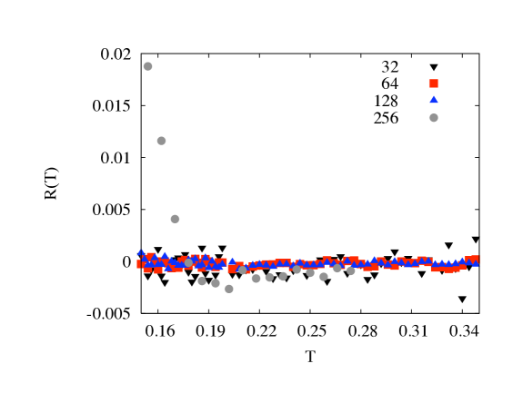
The results are very satisfactory for all temperatures up to $N=128$. For the largest system size however, the sampling is clearly not good enough below $T_{d}$, in spite of intensive numerical efforts. This is to be contrasted to the cases of the SK and Potts glass models where values of $N$ up to a few thousands can be handled with the parallel tempering algorithm [45, 20].

The modest efficiency of the parallel tempering algorithm when applied to the ROM can be directly observed by studying how the main thermodynamic observables reach their equilibrium values. Starting from a random initial configuration for the two clones (we take $\sigma_{i}=1,\forall i$), we plot the instantaneous value of the considered observable, averaged over the disorder, in order to tame the fluctuations. The results for the internal energy ($\overline{e(t)}$) and for the overlap between the two clones ($\overline{q(t)}$) are given in figure 2, for $T=0.178\simeq T_{d}$. This figure suggest a power-law behaviour $\overline{e}(t)-e_{\infty}\propto t^{-0.3}$ in the large $N$ limit, with a non uniform convergence. The smaller the value of $N$, the earlier in time do the data deviates from the power law behavior. For large $t$, the relaxation becomes strongly $N$ dependent, smaller systems relax much faster.

A power-law relaxation of the energy at $T_{d}$ is in fact expected on theoretical ground. The value of the exponent was recently conjectured by A. Lefèvre (private communication) to be equal to $a$, the MCT exponent defined above. This is compatible with our finding since, as we shall find later, $a\approx 0.35$ for the ROM.

Figure 2: Left: Relaxation of the disorder averaged internal energy from a random initial configuration, using the parallel tempering algorithm, for $N=64,128$ and $256$ at $T=0.178$, just above $T_{d}$. The apparent power law behavior $\overline{e}(t)-e_{\infty}\propto t^{-0.3}$ is only valid in the early time region. One notes that even (slightly) above $T_{d}$, the relaxation is extremely slow and equilibration is quite difficult to achieve (one needs a couple of $10^{5}$ Monte Carlo sweeps in order to equilibrate the internal energy for $N=256$). Right: Relaxation of the disorder averaged overlap between two clones from disordered initial configurations for $N=128$ and $256$ at $T=0.178$. The relaxation is much faster (a few hundred Monte Carlo sweeps are enough to equilibrate the overlap). We used the same color code of figure 1.

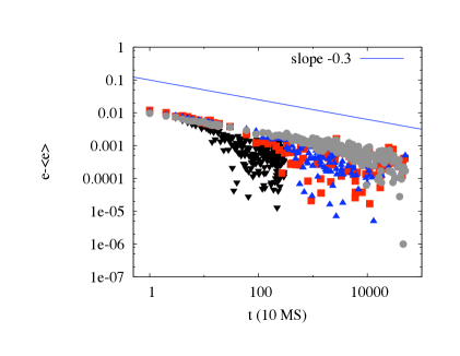
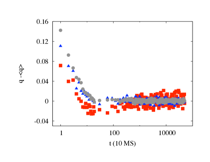
The slow relaxation of the internal energy, even for $T>T_{d}$, illustrates why this is a hopeless task to simulate the ROM below (and near) $T_{d}$ for reasonable system sizes. The much faster relaxation of the overlap can be understood with the following argument: the two clones starts at the top of a very rugged energy landscape. After a few sweeps, they have started falling down in directions, or towards, traps whose probable overlap is zero. This leads to a fast decorrelation of $\overline{q(t)}$. Instead, in order to equilibrate the internal energy, one has to visit many different traps in order to have a good statistical sampling of all energy states, which is a much more slow process.

Many reasons can be invoked to explain the poor performances of the parallel tempering algorithm applied to the ROM. The first one is that the temperature in the interesting region is in fact extremely low, leading to extremely small Metropolis and exchange acceptance rates. A way to gauge the smallness of the ROM transition temperature is to study the spin-glass susceptibility $\chi_{SG}=N\overline{\langle q^{2}\rangle}$ as a function of the temperature (see figure 3). When $T\to\infty$, $\chi_{SG}$ must tend to unity, but strong corrections are still present up to $T\approx 10T_{d}$. This is expected, since the leading non trivial $1/T$ correction to $\chi_{SG}$ is the same in the ROM and SK models, because the variance of the $J_{ij}$ is normalized to the same value in both cases. However, the critical temperature of the SK model is $T_{c}^{SK}=1$, ten times larger than the critical temperature of the ROM.

Figure 3: Spin-glass susceptibility for the ROM as a function of the temperature, for $N=32$ to $256$. One observes (a) strong size-dependence effect below $T_{d}\simeq 0.177$ and (b) an extremely slow convergence towards its asymptotic $T\to\infty$ value. In the inset $\chi_{SG}^{(N=32)}$ is plotted for high temperatures up to $35T_{s}$ together with the asymptote $\chi_{SG}^{(\forall N)}=1$. This illustrates how “cold” the ROM glassy phase is. We used the same color code of figure 1.

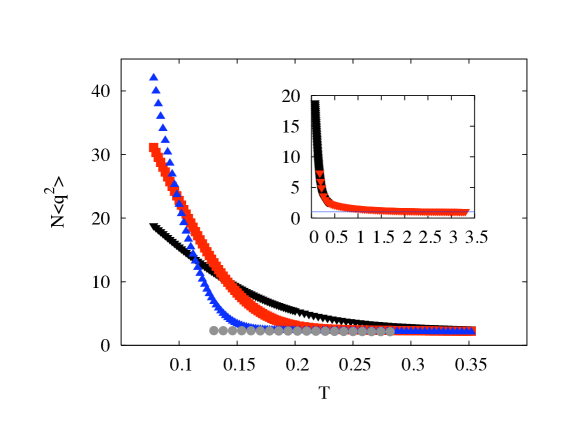
A deeper explanation relies on the physics of 1-RSB models, recalled in the above section. The existence of numerous metastable states in the range [$T_{s}$,$T_{d}$] slows down dramatically the dynamics. Indeed, in order to have a decent sampling, one should explore a representative subset of all the metastable states. The complexity of the ROM has been computed in the thermodynamic limit in [46]. It shows a sharp jump from $0$ to a finite value below $T_{d}$, and thus the log of the number of states that must be explored jumps from $0$ to a number of order $N$ at $T_{d}$. It does not come as a surprise that the algorithm fails below $T_{d}$ even for moderate values of $N$. A precise understanding of why the ROM case is so much difficult than the Potts and p-spin cases is still lacking. A reasonable conjecture is that this is due to fact that the overlap value is so close to unity. Another system where this happens, and where the dynamics is indeed painfully slow, is the Bernasconi model (see [47, 48]).

We note, en passant, that applied to the model with binarized exchange couplings briefly mentioned above, the parallel tempering works brilliantly.

3.4 Thermodynamics

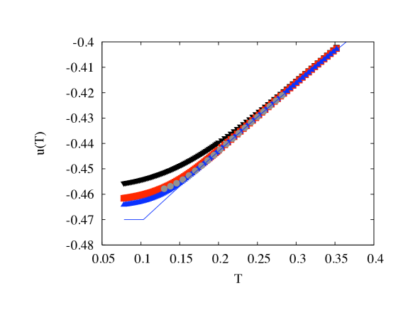
We show in figure 4 our data for the internal energy per spin, defined as $u(T)=\overline{\langle H\rangle}/N$ as a function of the temperature, together with the theoretical result obtained in [26]. For our special choice of $p$, one finds:

$$u(T) = \frac{1}{4}\left(T-\sqrt{T^{2}-\frac{3}{4}T+4}\right)\ ,\ T\geq T_{s}\ ,$$ (11)

$$u(T) = -0.47\ ,\ T<T_{s}\ .$$ (12)

The numerical data for $u(T)$ is qualitatively consistent with the infinite-volume analytical results, up to the finite size corrections, with the marked exception of the $N=256$ data below $T_{d}$, which are at odds with the rest of the picture. This is in agreement with our previous observation that the $N=256$ systems are not at equilibrium at low temperature and should be discarded there. The temperature below which the fluctuation-dissipation relation is violated indeed roughly coincides with the one below which the numerical values of $u(T)$ become manifestly wrong.

After discarding the bad data, $u(T)$ converges towards the predicted infinite-volume value, although with marked size-effects below the dynamical temperature. The finite size effects at $T=0.08$ are roughly compatible with a $1/N$ behavior. A similar observation was made for the p-spin model in [45].

Figure 4: Internal energy density $u(T)$ as a function of T for $N=32$ to $N=128$ (top to bottom) and $256$ (points that do not extend below $T=0.12$), together with the analytical prediction in the infinite volume limit.

Following [49], we plot in figure (5) the coefficient $A(T)$ defined as:

$$A(T)=\frac{\overline{\langle q^{2}\rangle^{2}}\ -\overline{\langle q^{2}\rangle}^{2}}{\overline{\langle q^{2}\rangle}^{2}}\ ,$$ (13)

that signals [50] the onset of the non self-averaging behavior of $q^{2}$. In figure 5, we plot the usual Binder parameter,

$$B(T)=\frac{1}{2}\left(3-\frac{\overline{\langle q^{4}\rangle}}{\overline{\langle q^{2}\rangle}^{2}}\right)\ .$$ (14)

Figure 5: The parameter $A$ (left) and the Binder parameter $B(T)$ (right) as a function of $T$, for$N=32$ to $256$. We used the same color code of the previous figures.

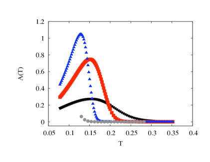
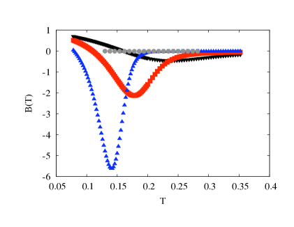
For generic 1-RSB transitions, Picco et al. [49] have argued that these two coefficients are zero for $T>T_{s}$ (in the thermodynamic limit), non zero for $T<T_{s}$ and in fact diverge at the static transition $T\to T_{s}^{-}$. The fact that the Binder coefficient is negative when $T\to T_{s}^{-}$ is simply related to the appearance of a peak in $P(q)$ for $q\neq 0$. In the infinite volume limit, one has:

$$P(q)=(1-m)\delta(q)+m\delta(q-q_{1}),$$ (15)

with $m<1$, and $m\to 0$ when $T\to T_{s}^{-}$. Accordingly one has $B(T)=1/2(1-1/m)<0$ in the 1-RSB region.

Our data are in qualitative agreement with the above limiting behavior (see [49, 17] for a similar numerical analysis in the case of the p-spin model). Note that for a 1-RSB transition, the curves of $B(T)$ as a function of $T$ for various values of $N$ do not cross at a universal point, at variance with usual phase transitions (including $\infty$-RSB transitions).

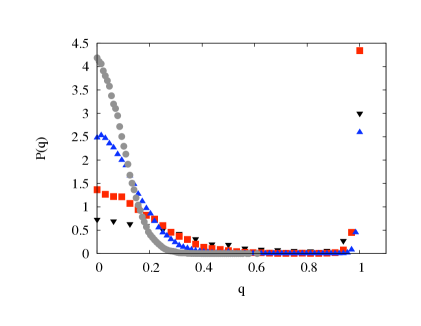
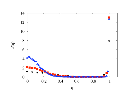
The overlap probability distribution $P(q)$ is found to have the shape corresponding to a 1-RSB phase transition, with one peak around $q=0$ and, below $T_{s}$, another peak around $q=q_{1}$ ($q_{1}$ is close to one in our specific case). With $N$ finite, both peaks have a non zero width, as always. It turns out that the $q=0$ peak is much broader that the peak at $q=q_{1}$. Above $T_{s}$, our data shows a spurious peak centered at $q\simeq 1$. This peak however corresponds to an unstable thermodynamic phase and decays sharply with the size of the system (see figure 6) as it should. As shown in figure (6), the peak centered at $q\simeq 1$ becomes extremely sharp for $T<T_{s}$ .

Figure 6: Left: $P(q)$ for $T_{s}<T=0.154<T_{d}$.. Right:$P(q)$ for $T=0.078<T_{s}$. Both for $N=32$ to $128$. We used the same color code of the previous figures.

3.5 Thermodynamics: Conclusion

We have thus been able to confirm numerically the main replica predictions for the ROM: the energy as a function of the temperature freezes at the static transition, and the order parameter is strongly discontinuous there. This could be related to the fact that the static transition temperature is very small, compared, for example, to the SK model. Correspondingly, it is very hard to equilibrate the system despite intensive numerical efforts. Systems with $N=256$ did not reach equilibrium below the dynamical transition.

4 Numerical Simulations: dynamical behavior

We now present our numerical study of the equilibrium dynamics of the ROM. On theoretical grounds, and in view of the above results on the statics of the model, the dynamics of the ROM should be described by the Mode-Coupling Theory, at least in a Landau sense, i.e. the MCT power laws are expected to be valid and the actual values of the exponent, although not universal, are constrained to verify equations 2 and4, see[9]) We compare our data with the predictions of MCT both for the two-point and four-point correlation functions. The results are very puzzling at first sight. We will show in the following sections that a detailed understanding of preasymptotic corrections and finite size effects is required in order to rationalize our numerical results.

4.1 Dynamic scaling and comparison with MCT

We first focus on the dynamical overlap $q_{d}(t)$ (defined in equation 1). Our data show a plateau in $q_{d}(t)$, whose extension increases by lowering the temperature, see Fig 7.

Figure 7: Left: Dynamical overlap $q_{d}(t)$ for the largest system ($N=256$), and for various temperatures from $T\simeq T_{d}$ (upper curve) to $T=1.65\ T_{d}$ (The temperature step is such that $\Delta T/T_{d}=5\%$).Right: Test of Time-Temperature superposition for $q_{d}(t)$ for all sizes ($N=256$ grey circle, $128$ blue upper triangle, $64$ red squares and $32$ black lower triangle) and various temperatures from $T=1.25\ T_{d}$ to $T=1.65\ T_{d}$. One remarks clearly the decay of finite-size corrections and the convergence to a limiting curve.

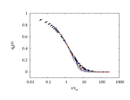
The value of the dynamical overlap on the plateau is close to the infinite-volume limit of the Edwards–Anderson parameter ($q_{EA}(T_{d})\approx 0.955$), as it should. After a single Monte Carlo sweep, $q_{d}(t)$ has already decayed to the plateau value. Therefore we cannot observe the early $\beta$-regime. This is an unfortunate drawback of our choice of the ROM with parameter $p=13/32$. We however do see the $\alpha$ regime in full glory. Our results are quite different from those obtained for the Potts model [20, 21, 22], where no plateau was observed in $q_{d}(t)$ for systems with up to $N=2560$.

In order to be quantitative, we define the time scale $\tau_{\alpha}(T)$ (see equation 3) as the time needed to reach the value $q_{d}(\tau_{\alpha})=1/2$. If Time-Temperature superposition (TTS) holds, the precise definition used is irrelevant. We have checked that the $q_{d}(t)$’s plotted as a function of $t/\tau_{\alpha}(T)$ approximately collapse on a unique scaling curve for the largest system sizes, but for temperatures not too close to $T_{d}$, see Fig 7.

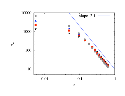
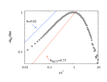
However, as $T$ gets closer to $T_{d}$, TTS appears to breakdown: instead of approaching a universal scaling curve, the $q_{d}(t)$’s are more and more stretched as the system size increases. This is a priori surprising since TTS should work better close to the MCT transition. But we find that close to $T_{d}$, finite size effects become important. This is also revealed by the behavior of $\tau_{\alpha}(T)$ as a function of $\epsilon=(T-T_{d})/T_{d}$, see Fig 8. A MCT power law fit, $\tau_{\alpha}\propto\epsilon^{-\gamma}$, accounts reasonably well for the regime $\epsilon>0.2$ where finite size effects are small, and yields $\gamma\approx 2.1$. MCT also makes detailed prediction about the form of the scaled relaxation function, as we discussed in the introductory sections. Unfortunately the power-law predicted in the early $\beta$ regime is inaccessible because the plateau is too close to unity. However, we can check the (von Schweidler) power-law associated to the late $\beta$ regime. In order to do so in a way that does not require a precise determination of the plateau value $q_{EA}$, we plot in figure 8 $-dq_{d}/d\ln t$ for our largest system size $N=256$ at the lowest temperature at which we do not have substantial finite size effects. According to MCT, this quantity should increase as $t^{b}$ when $\tau_{\beta}\ll t\ll\tau_{\alpha}$. From the power law fit shown in figure 8 we determine $b\approx 0.62$. But within MCT the values of $b$ and $\gamma$ are not independent (see equations (2,2) above). The value of $b$ corresponding to $\gamma\approx 2.1$ is found to be $b_{MCT}\approx 0.75$ which is distinctly too large compared to our data (see Fig 8). This is a second puzzling result since MCT predictions are expected to apply to the ROM dynamics close to $T_{d}$.

Figure 8: Left: Relaxation times $\tau_{\alpha}$ versus $\epsilon=(T-T_{d})/T_{d}$, for different system sizes (same color code of previous figures). For $\epsilon>0.2$, i.e. $T>1.2\ T_{d}$, an $N$-independent regime is observed, with $\tau_{\alpha}\propto\epsilon^{-\gamma}$ and $\gamma\approx 2.1$, over two time decades. Right: Determination of the $b$-exponent of the von Schweidler law through the derivative of the overlap, $-dq_{d}/d\ln t\propto t^{b}$. (Here $N=256$, $T=0.226$). The two straight lines correspond to $b=0.62$ and $b_{MCT}=0.75$ respectively.

Other puzzling features emerge from the analysis of the dynamic susceptibility $\chi_{4}(t)$, as defined by equation (5). A plot of the peak value $\chi_{4}^{*}$ as a function of $\epsilon$ for our largest system size shows (in the regime without finite size effects) a power law behavior compatible with the MCT prediction $\chi_{4}^{*}\propto 1/\epsilon$ (see figure 9). However, figure 9 shows that there is no collapse of $\chi_{4}(t)/\chi_{4}^{*}$ plotted as a function of $t/\tau_{4}$, where $\tau_{4}$ is such that $\chi_{4}^{*}\equiv\chi_{4}(t=\tau_{4}$), at variance with the MCT prediction for $t<\tau_{4}$ . Before the peak, $\chi_{4}(t)$ appears to grow as $t^{b_{4}}$ with $b_{4}\approx 0.85$. Such a power-law increase is again predicted by MCT, but one should find $\chi_{4}(t)\propto-dq_{d}/d\ln t$ [10, 11], i.e. $b_{4}=b\approx 0.62$. In fact, MCT also predicts that $\chi_{4}(t)\propto-dq_{d}/dT$ [14]. We show in figure 10 these three different quantities in log-log plot. Although $-dq_{d}(t)/dT$ and $-dq_{d}/d\ln t$ are indeed similar, $\chi_{4}(t)$ does not conform to expectations.

Figure 9: Left: Maximum of $\chi_{4}$ versus $\epsilon$. The MCT prediction would be $\chi_{4}^{*}\propto 1/\epsilon$. Right: Scaling plot for $\chi_{4}$ (here N=256). The straight line corresponds to a power law with an exponent $0.9$.

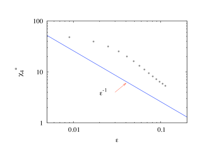
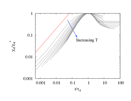
In conclusion: although some of the MCT predictions are quantitatively obeyed, other important ones are clearly violated. The solution of this conundrum is that the values of $\epsilon$ used above are actually not small enough to be in the asymptotic regime where MCT predictions hold. As we shall show in the next section, these predictions are only valid in a surprisingly small region close to the transition. So why not work closer to $T_{d}$? The next problem we will have to deal with (section 5) is finite size effects, that become large close to $T_{d}$. Therefore, only after a very careful finite size analysis can one conclude on the compatibility between the MCT predictions and the numerical behavior of a model that is in principle exactly described by MCT! We will show how difficult this program turns out to be for the ROM. This sheds considerable doubt on the precise, quantitative comparison between experimental data and MCT, since these problems should show up in these cases as well.

Figure 10: Comparison of three susceptibilities: $\chi_{4}$ (circles), $-dq_{d}/d\ln t$ (squares) and $-dq_{d}/dT$ (triangles). Here, $N=256$ and $T=0.226$. Each susceptibility has been rescaled with its own $\chi^{*}$ and $\tau^{*}$. All three quantities should grow with the same initial power-law behavior within MCT. This is clearly not the case for $\chi_{4}$(t).

4.2 MCT critical properties and preasymptotic corrections

At this stage, it is important to have a reliable reference point to which we can compare our numerical results. For this we choose to study in detail the Leutheusser integro-differential equation for the correlation function [51], which comes out of the schematic version of MCT with a so-called quadratic kernel:

$$\ddot{\Phi}(t)+\Omega\dot{\Phi}(t)+\Phi(t)+4\lambda\int_{0}^{t}d\tau\Phi^{2}(\tau)\dot{\Phi}(t-\tau)=0,\hskip 14.22636pt\Phi(0)=1$$ (16)

In the above equation, $\Phi(t)$ is the correlation function and plays the role of $q_{d}(t)$ above, and $\lambda$ is the coupling constant that measures the strength of the feedback effects at the heart of the MCT transition. Remarkably, the equation above is also the one governing the evolution of the correlation function for the $p=3$ mean field disordered p-spin model [28]. It can be analyzed mathematically, and all the results quoted in section 2 can be shown to hold exactly in the limit $\lambda\to\lambda_{d}=1$. In particular, the model is ergodic for $\lambda<1$, where $\lim_{t\to\infty}\Phi(t)=0$, and develops power-law regimes with exponents $a$ and $b$ given by (equation 2):

$$\frac{\Gamma^{2}(1+b)}{\Gamma(1+2b)}=\frac{\Gamma^{2}(1-a)}{\Gamma(1-2a)}=\frac{1}{2},$$ (17)

leading to $a\approx 0.315$, $b=1$, $\gamma\approx 1.765$.

The Leutheusser equation can be solved numerically for arbitrary large values of $t$, using for example the algorithm of [52]. In what follows we fix $\Omega=1$, and neglect the $\ddot{\Phi}(t)$ term, as usually done. In order to compare directly with the ROM data above, we have computed $\Phi(t)$ for values of $\lambda$ that are at the same relative distances from the critical point as our ROM data, for temperatures $T=0.178,0.186,\ldots$, and $0.250$. (We recall that $T_{d}=0.177$ for the ROM.)

Figure 11: Leutheusser model. Left: Scaling plot of $\Phi(t)$ as a function of $t/\tau_{\alpha}$, at the same relative distances from the MCT transition as for our ROM data above $T_{d}$, namely $\lambda=T_{d}/T$, for $T=0.178,0.186,\ldots,0.250$. The $\alpha$ time scale is given by $\tau_{\alpha}=(1-\lambda)^{-1.765}$. Right: Scaling plot of $-d\Phi(t)/d\ln t$. The expected late $\beta$ behavior $t^{b}$ with $b=1$ is shown for comparison. The straight line represents $y=t/(5\tau_{\alpha})$.

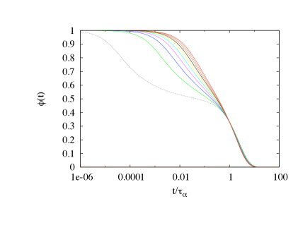
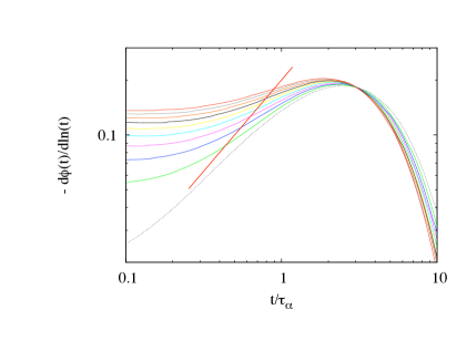
Figure 11 shows a TTS plot of $\Phi(t)$ using the exact value of $\gamma$, i.e. using $\tau_{\alpha}=\epsilon^{-1.765}$, where $\epsilon=(1-\lambda)=(T-T_{d})/T_{d}$. This figure shows apparent scaling in the late $\beta$ (von Schweidler) regime, with only small scaling violation. However, only the relaxation corresponding to the value of $\lambda$ closest to unity ($\epsilon\approx 0.05$) reveals the expected two-step relaxation with a nontrivial plateau region!

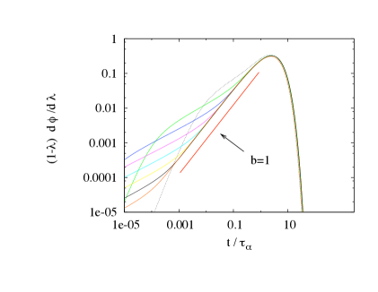
More revealing is a log-log plot of $-d\Phi(t)/d\ln t$, shown in figure 11 together with the expected theoretical behavior $-d\Phi(t)/d\ln t\propto t^{b}$ with $b=1$ (The derivative is computed by plain finite difference). We now see very strong scaling violations before the peak, and an apparent value of $b$ that is significantly below $1$, even for the curve closest to the critical point. The conclusion is that while the value of $\gamma$ extracted from a TTS plot of $\Phi(t)$ is reasonable, the value of $b$ that one can extract from $\Phi(t)$ $5\%$ away from the critical point is grossly underestimated. This is similar to our observations above for the ROM.

Let us now turn to the non linear susceptibilities $\chi_{4}(t)$ and $\chi_{T}(t)=d\Phi(t)/d\lambda$. Within MCT, both quantities have the same scaling behavior. In particular one expects that $\chi_{4}(t)=\epsilon^{-1}F(t/\tau_{\alpha})$, with $F(x)\propto x^{b}$, in the late $\beta$ regime. Numerically, $\chi_{T}(t)$ is easy to obtain from the value of $\Phi(t)$ for different values of $\lambda$. The case of $\chi_{4}(t)$ is less straightforward. It turns out [12] that a dynamical susceptibility, proxy of $\chi_{4}(t)$, can be computed for the spherical p-spin model, which as recalled before is characterized by a dynamical equation for the correlation function identical to the the one of the Leutheusser model. A perturbed-time dependent Hamiltonian $H_{\eta}$ is introduced:

$$H_{\eta}=H-\eta q_{d}(t)$$ (18)

where $H$ is the usual p-spin Hamiltonian, and $q_{d}(t)$ is the overlap between the spin configurations at times $t$ and $t=0$. Then $\chi_{4}(t)\equiv d\langle q_{d}(t)\rangle/d\eta\Bigr{|}_{\eta=0}$. For a given value of $\eta$, one is led to a set of two integro differential equations that can be solved numerically [53]. The estimate of $\chi_{4}(t)$ follows from a careful extrapolation to $\eta=0$.

Figure 12: Left: Scaling plot of $\chi_{T}(t)=d\Phi(t)/d\lambda$. The values of $\lambda$ are the same as in figures 11, with the same color code. The expected scaling behavior $d\Phi(t)/d\ln\epsilon\propto(t/8\tau_{\alpha})^{b}$ with $b=1$ is shown for comparison. Right: Scaling plot of $\chi_{4}(t)$ for the spherical 3-spin model, with again the same values of $\epsilon$ and the same color code. The straight line corresponds to the theoretical prediction $\chi_{4}\propto\epsilon^{-1}(t\epsilon^{\gamma})^{b}$.

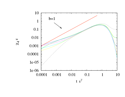
Figures 12 shows scaling plots for $\chi_{T}(t)$ and $\chi_{4}(t)$. Although an approximate scaling is observed close to the peak, only the $\chi_{T}(t)$ curve closest to the transition gives a hint of the correct value of the exponent $b$. The scaling violations are non monotonous and can fool the reader into seeing scaling with some $b$ less than the correct value. The estimate for $b$ from $\chi_{4}(t)$ is systematically larger, and closer to the true value. This again is similar to our numerical observations for the ROM.

In order to observe the asymptotic MCT scaling predictions, one must work much closer to the transition. For example, the expected linear regime of $-d\Phi(t)/d\ln t\propto(t/\tau_{\alpha})$ only appears very slowly as $\lambda\to 1$, and is well developed only for $\epsilon\leq 10^{-4}$. Figure 13 shows a similar behavior for $d\Phi(t)/d\lambda$. The linear region appears only when $\epsilon\leq 10^{-3}$. Finally figure 13 shows the even slower approach to scaling of $\chi_{4}(t)$ (beware however that $\epsilon$ is here limited to $10^{-6}$).

Figure 13: Same as figure 12, but going deeply inside the scaling region, namely for $\epsilon=10^{-1},10^{-2},\ldots,10^{-8}$ for the left wing figure, $\epsilon=10^{-1},10^{-2},\ldots 10^{-6}$ for the right wing figure. The straight line are the same as in figure 12.

4.3 Dynamics: Conclusion

The above results show that the true asymptotic regime of MCT is unusually narrow. This should be remembered when comparing numerical (or experimental) data with MCT predictions. These data are usually plagued with noise and possible finite size effects, on top of the strong scaling violations that appear even in the best case situation studied in this section. On the other hand, some useful conclusions emerge, which allows us to make sense of our data on the ROM dynamics in the preasymptotic regime: (i) an approximate TTS holds for the late $\beta$ regime, with the correct value of exponent $\gamma$; (ii) the exponent $b$ extracted from the time dependence of the correlation function underestimates the true value; (iii) for the dynamical susceptibility $\chi_{4}$, the scaling is acceptable around the peak with the predicted divergence $\epsilon^{-1}$, with a value of $b$ in the correct range. From these considerations, we conclude that the correct values of $b$ for the ROM should be around $b\approx 0.8$, and the corresponding value of $\gamma$ close to $2$, and $a\approx 0.35$. A confirmation of these values should come from studying the dynamics closer to $T_{d}$. However, finite size corrections become important there and we now turn to the study of these effects.

5 Finite-Size Scaling: More surprises

In the previous section, we have shown that the critical behavior of the ROM dynamics in the regime where finite size corrections are small is polluted by strong preasymptotic effects. In order to get rid of those one should simulate very large systems very close to $T_{d}$, which is alas not possible since the equilibration time also becomes very large. The hope would be to use finite size scaling (FSS) to extract the interesting asymptotic behavior.

5.1 Naive theory and comparison with numerical data

The MCT predictions are modified for finite but large system sizes. One expects in particular that activated effects, absent for infinitely large systems, start playing a role for finite systems close to $T_{d}$.

As we have recalled above, it was recently recognized that MCT is a mean field (Landau) theory characterized by a diverging length scale $\xi\propto\epsilon^{-1/4}$ [10, 11] and the corresponding upper critical dimension is $d_{u}=6$. Assuming that the field theoretical analysis of [54, 55] applies also to this dynamical transition we expect that finite size scaling holds for MCT above the upper critical dimension $d_{u}$ where the proper scaling variable is not $L/\xi=N^{1/d}\epsilon^{\nu}$ but rather $N^{1/d_{u}}\epsilon^{\nu}$ [56]. The fully connected ROM is obviously above the upper critical dimension and the relaxation time $\tau_{\alpha}$ for a finite system should therefore take the following scaling form:

$$\tau_{\alpha}(T,N) = N^{\frac{\gamma}{\nu d_{u}}}\mathcal{F}(N^{\frac{1}{\nu d_{u}}}\epsilon),\qquad\nu d_{u}=3/2$$ (19)

When $N\to\infty$, all $N$ dependence should disappear and the MCT divergence of equation(4) must be recovered. This means that the scaling function $\mathcal{F}$ must behave as $\mathcal{F}(x)\propto x^{-\gamma}$ when $x\gg 1$.

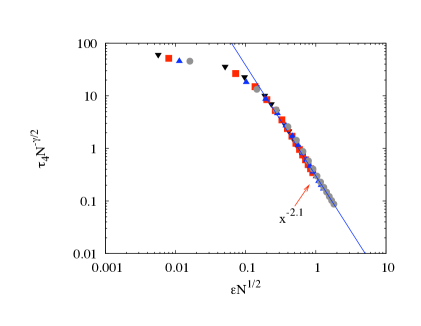
We analyze our numerical results on $\tau_{\alpha}(T,N)$ using the above FSS form, see Fig 14. A good collapse of the different curves can indeed be obtained using equation (19) with $\gamma=2.1$, but we need to use the value $d_{u}\nu=2$ instead of the expected value $3/2$.

Figure 14: Left: Scaling plot of $\tau_{\alpha}(T,N)$ using equation (19) with $\gamma=2.1$ and $d_{u}\nu=2$. Right: Scaling plot of the maximum of $\chi_{4}$, using equation (20) with $d_{u}\nu=2$ and $s=1$.

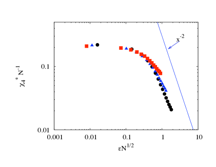
If we now turn to the four-point susceptibility $\chi_{4}$, another confusing result is obtained. While the peak location $\tau_{4}^{*}$ has the same finite size scaling as $\tau_{\alpha}$, as expected, the FSS of the peak height should read:

$$\chi_{4}^{*}(T,N) = N^{s}\mathcal{G}(N^{\frac{1}{\nu d_{u}}}\epsilon).$$ (20)

Using the above effective value $\nu d_{u}=2$, the exponent $s$ should be such that for large $N$, $\chi_{4}^{*}$ diverges as $\epsilon^{-1}$ independently of $N$. This fixes $s=1/2$, at variance with our numerical data that suggests $\chi_{4}^{*}\propto N^{s}$ with $s\simeq 1$, see figure 14. Note that despite the uncertainties on the exact value of $s$, we clearly find that $s>1/2$ (note also the decay of the scaling function $\mathcal{G}(x)$ at large arguments).

We therefore find that finite size scaling appears to work for the ROM transition but not in the way expected, at least naively. In particular, the scaling variable $\sqrt{N}\epsilon$ is at odds with the value of the upper critical dimension for the ROM dynamics (without explicitly conserved variables) and the value of the exponent $\nu$.

The next sections are dedicated to a detailed discussion and explanation of these puzzling results. As we shall show there is no contradiction whatsoever and the origin of this strange FSS are sample to sample fluctuations of the critical temperature $T_{d}$.

5.2 Harris criterion and random critical points

It is well known that the stability of pure critical points with respect to weak disorder [57] is governed by the Harris criterion: near a second order phase transition in dimension $d$, the bond disorder is irrelevant if the specific heat exponent $\alpha_{pure}=2-d\nu_{pure}$ is negative, where $\nu_{pure}$ is the correlation length exponent of the pure system. Then the critical exponents of the disordered system are the same as the ones of the pure system.

If $\alpha_{pure}>0$, disorder becomes relevant and the system is driven towards a so called random fixed point characterized by a new correlation length exponent $\nu_{R}$ satisfying the general bound $\nu_{R}\geq 2/d$. In the last twenty years, important progress [58, 59, 60] has been made in the understanding of finite size properties of random critical points. For our purpose we only recall that to each realization of disorder ($\omega$), one can associate a pseudo-critical temperature $T_{d}(\omega,N)$, defined for instance as the temperature where the relevant susceptibility is maximum. The disorder averaged pseudo-critical critical temperature $T^{N}_{d}\equiv\overline{T_{d}(\omega,N)}$ converges towards its infinite size limit as: $T^{\infty}_{d}-T_{d}^{N}\propto N^{-1/d\nu_{R}}$. The width $\Delta T_{d}(N)$ of the distribution of the pseudo-critical temperatures $T_{d}(\omega,N)$ then depends on the nature of the critical point. If the disorder is irrelevant, $\Delta T_{d}(N)$ scales trivially like $N^{-1/2}$, but like $N^{-1/d\nu_{R}}$ if the disorder is relevant.

Figure 15: Sketch of the sample to sample fluctuations of a susceptibility in situations where the critical temperature fluctuates on scales $N^{-1/2}$, much larger than the FSS thermal window $N^{-2/3}$. Here $\omega$ and $\xi$ are two disorder configurations.

All previous studies of FSS for disordered systems mentioned above have focused on models below their upper critical dimension (see for example [61]). Instead the ROM is clearly above its upper critical dimension. As a consequence, it is not obvious to deduce its FSS behavior from previous works. In A we discuss in detail the subtleties of the Harris criterion above the upper critical dimension.

From a phenomenological point of view, one expects that general features of random fixed points should still occur: in particular one can define a sample-dependent pseudo-critical dynamical temperature $T_{d}(\omega,N)\equiv T_{d}+\delta T(\omega,N)$. A hand-waving argument to understand the origin of these fluctuations is to consider the TAP equations for the ROM. The high temperature expansion leading to the TAP equations for the ROM has disorder-dependent corrections of order $N^{-1/2}$. These have a dramatic effect on FSS since these corrections are much larger than the expected FSS thermal window $N^{-2/3}$ of the MCT-transition. We will therefore assume, and justify later on, that for each sample the FSS window is indeed of the order $N^{-2/3}$ around a random critical temperature that has disorder fluctuations of the order $N^{-1/2}$. As a consequence, FSS for disordered averaged observables are dominated by the fluctuations of the critical temperature that wash out the much sharper $N^{-2/3}$ FSS thermal window  (see figure 15 for a cartoon representation). Note that a similar situation for FSS of random first order transition has been discussed by D.S. Fisher in [62].

5.3 Random critical temperatures and modified FSS

To make the above statements more precise, let us consider the generic example of some thermodynamic observable $\mathcal{O}$. One would like to compute $\overline{\mathcal{O}}$. We assume that averaging over the disorder is equivalent to averaging over the distribution of critical temperatures, $p(T_{d}(\omega,N))$. For the sake of simplicity, $p(T_{d}(\omega,N))$ is taken to be a well behaved distribution with width of order $N^{-1/2}$ centered on $T_{d}$, the true asymptotic dynamical temperature . Moreover, we posit that for each sample, some kind of FSS holds, in the sense that:

$$\mathcal{O}(T,N)=N^{2\zeta/3}\mathcal{F}(N^{2/3}[T-T_{d}(\omega,N)])$$ (21)

where $\zeta$ is a certain exponent that depends on the particular observable, and the scaling function $\mathcal{F}$ is, at least to leading order, sample-independent. We assume that $\mathcal{F}(x)$ is regular for small arguments, and $\mathcal{F}(|x|)\propto A_{\pm}|x|^{-\zeta}$ for $x\to\pm\infty$, such that $\mathcal{O}(T,N\to\infty)\propto|\epsilon|^{-\zeta}$ independently of $N$. It is possible to justify all these assumptions within a simple toy model, the weakly disordered version of the Blume-Capel model, that displays exactly the unusual FSS discussed in this section. We warmly invite the reader to examine B for more details.

Now, writing $T_{d}(\omega,N)=T_{d}-yN^{-1/2}$, disorder averaging is obtained by computing:

$$\overline{\mathcal{O}}(T) = N^{2\zeta/3}\int dy\,p(y)\mathcal{F}(N^{2/3}\epsilon+N^{1/6}y)$$ (22)

where $\epsilon=T-T_{d}$. The analysis of the above integral in the large $N$ limit requires to distinguish two cases: $\zeta<1$ and $\zeta>1$ (with further logarithmic terms when $\zeta=1$).

• When $\zeta<1$, one can set $\epsilon=u/\sqrt{N}$ and take $N\gg 1$ in the above integral, to get to leading order:

  $$\overline{\mathcal{O}}(T) = N^{\zeta/2}\hat{\mathcal{F}}(\sqrt{N}[T-T_{d}]),$$ (23)

  $$\hat{\mathcal{F}}(u) = \int_{-u}^{\infty}dy\,\frac{A_{+}p(y)}{(u+y)^{\zeta}}+\int_{-\infty}^{-u}dy\,\frac{A_{-}p(y)}{|u+y|^{\zeta}}$$ (24)

  Since $\zeta<1$, the integral defining $\hat{\mathcal{F}}$ is always convergent when $u\to 0$, leading to a well behaved scaling function. Therefore, in this case the usual FSS strategy is valid, with a scaling variable dominated by the fluctuations of critical temperature: $N^{2/3}\to N^{1/2}$.

• When $\zeta>1$, on the other hand, the relevant change of variable is $y=z/N^{1/6}-u$. Again to leading order, this gives:

  $$\overline{\mathcal{O}}(T) \approx AN^{\frac{4\zeta-1}{6}}p\left(-\sqrt{N}[T-T_{d}]\right)$$ (25)

  where $A=\int dz\,\mathcal{F}(z)$ is a convergent integral thanks to the rapid decay of $\mathcal{F}(z)$ for large $z$, leading to a finite multiplicative constant. In this case, FSS is drastically altered by the sample to sample fluctuations of the dynamical temperature; the decay of the scaling function is related to the one of the distribution of critical temperatures, and the exponent ${(4\zeta-1)}/{6}$ is unusual.

The above analysis can be extended to the case of “assymetric observables”, where the power-law decay of $\mathcal{F}(x)$ is different when $x\to+\infty$ and $x\to-\infty$. Most of the interesting ROM observables turn out to be of that type around $T_{d}$, see section 5.5, 5.6.

5.4 FSS for single samples

Figure 16: Left: $\tau_{\alpha}$ is plotted as a function of the temperature for 5 different disorder samples ($N=32$ with $N_{ther}=120$ only). There are clear strong sample to sample fluctuations of the relaxation time. Close to $T_{d}$, the five curves can be superposed by a suitable horizontal shift, namely one has the relation $\tau(\omega,N)=\mathcal{C}(T-T_{d}(\omega,N))$. Right: Scaling plot of the relaxation time $\tau_{\alpha}$ using rescaled sample dependent dynamic temperature. Here are plotted the fastest, the slowest and a typical sample for all sizes (N=256 corresponds to grey circle, N=128 to upper blue triangle, N=64 to red squares and N=32 to lower black triangle). We recovers the standard FSS exponents by using $T_{d}(\omega,N)$ instead of the thermodynamic $T_{d}$

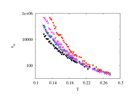
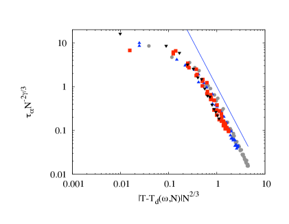
Checking these assumptions numerically is tricky for the ROM. If there was a quantity (susceptibility-like) with a sharp peak around $T_{d}$ then it would be simple: one would just rescale for each sample this quantity around its peak and verify whether the usual finite size scaling holds, as suggested by figure 15. Unfortunately, no such quantity exists for the ROM. As we have seen, $\chi_{4}^{*}(T)$ is a monotonously decreasing function of temperature. In order to check the usual FSS, one should shift horizontally $\chi_{4}^{*}(T)$ for each samples around its own effective dynamical transition temperatures $T_{d}(\omega,N)$. In order to determine this effective critical temperature we focus on the sample to sample fluctuations of the relaxation time (see left panel of figure 16). We assume that the relaxation time is uniquely determined —at fixed $N$— by the distance $T-T_{d}(\omega,N)$, i.e. $\tau(\omega,T)=\mathcal{C}(T-T_{d}(\omega,N))$, where $\mathcal{C}$ is a certain function. Thus, choosing a certain reference relaxation time $\tau^{*}$ for a given sample, one fixes the difference $T^{*}(\omega,N)-T_{d}(\omega,N)$ to a sample independent value $\delta^{*}$ (with $\tau(\omega,T^{*}(\omega,N))=\tau^{*}$) . Therefore, by averaging,

$$\delta^{*}=T^{*}(\omega,N)-T_{d}(\omega,N)=\overline{T^{*}(\omega,N)-T_{d}(\omega,N)}=\overline{T^{*}(\omega,N)}-T_{d}+O(N^{-2/3}),$$

where we have assumed that the $N$ dependent correction to the average critical temperature is $O(N^{-2/3})$, that only introduces a shift in the final scaling variable. The above equation allows one to determine the sample dependent shift of critical temperature, $T_{d}(\omega,N)-T_{d}$, as ${T^{*}(\omega,N)}-\overline{T^{*}(\omega,N)}$. This procedure does not require the knowledge of the functional form of the relaxation time. Once this shift is know, one can rescale the temperature axis in a sample dependent way, and test FSS sample by sample.

Figure 17: Scaling plot of the maximum of $\chi_{4}$ with sample dependent transition temperatures $T_{d}$ (same convention as figure 16). The behavior of $\chi_{4}^{*}(T)$ is now compatible with the MCT-predictions, $\chi_{4}^{*}(T)\propto\epsilon^{-1}$ and with the standard finite-size scaling exponents.

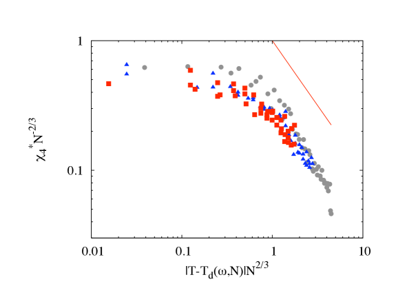
The results are given in figures 16 and 17. Our statistics is quite limited because of the CPU-time consumption of such simulations. The modest number of thermal configuration does not allow us to extract the whole probability distribution for $T_{d}(\omega,N)$. Despite these limitations, the results are in perfect agreement with our expectations. After the above temperature rescaling, the best collapse of the relaxation time data is obtained with the naive finite-size scaling ($N^{2/3}(T-T_{d}(\omega,N)))$ and not $\sqrt{N}(T-T_{d}(\omega,N))$. A similar behavior is obtained for $\chi_{4}^{*}$. The dynamical susceptibility divergence is now compatible with an $\epsilon^{-1}$ behavior derived analytically for MCT transition.

5.5 Anomalous FSS for the dynamical susceptibility

Now we are confident in the validity of our analysis in terms of sample dependent transition temperatures, we come back on the anomalous FSS properties of the dynamical susceptibility that we observed numerically in section 5.1 above. We must first guess the shape of the sample dependent FSS for the peak susceptibility. When $T>T_{d}(\omega,N)$, we expect a divergence of $\chi_{4}^{*}(T)$ as $\epsilon^{-1}$, as discussed in the section above. So the exponent $\zeta_{+}$ corresponding to this region is $\zeta_{+}=1$. On the other hand, below the transition one expects that the variance of the dynamical overlap will be of order $N$, due to activated dynamics that makes the system hop between states with zero mutual overlap (see the above remark on the fast relaxation of $q_{d}(t)$ in the ROM). Matching the requirement $\chi_{4}^{*}(T)\propto N$ with the finite-size scaling form valid near $T_{d}(\omega,N)$, $\chi_{4}^{*}(T)\approx N^{2/3}\mathcal{F}(N^{2/3}(T-T_{d}(\omega,N)))$ leads to $\mathcal{F}(x)\sim\sqrt{-x}$ for $x\to-\infty$, or $\zeta_{-}=-1/2$. Extending the analysis of section 5.3 to this strongly asymmetric case where $\zeta_{+}\neq\zeta_{-}$, we find that the average behavior is dominated by the left tail of $\mathcal{F}(x)$, finally leading to:

$$\chi_{4}^{*}(T) \sim N^{s}\mathcal{G}(\sqrt{N}(T-T_{d})),$$ (26)

where the anomalous exponent $s$ is equal to $3/4$ and $\mathcal{G}$ is a certain scaling function. We therefore qualitatively understand the anomalous FSS result obtained in section 5.1, in particular the fact that $s$ is larger than the naive value $s=1/2$.

5.6 Relaxation time: some conjectures

We finally turn to the relaxation time $\tau_{\alpha}$, which, as we already know, is very strongly sample dependent. The guess for the sample dependent FSS of the relaxation time must now account for the $\epsilon^{-\gamma}$ divergence for $T>T_{d}(\omega,N)$, and the activated dynamics for $T<T_{d}(\omega,N)$. If we assume that the relevant energy barrier scales with the system size as $N^{\psi}$, one is led to the following ansatz:

$$\tau(\omega,N) = N^{\frac{2\gamma}{3}}\mathcal{F}((T-T_{d}(\omega,N))N^{\frac{2}{3}}),\mbox{with}$$ (29)

$$\mathcal{F}(x)\propto\exp(-C(\omega)|x|^{\frac{3\psi}{2}})\ \ \ x\to-\infty$$

$$\mathcal{F}(x)\propto x^{-\gamma}\ \ \ x\to\infty,$$

where $C(\omega)$ is a sample dependent constant that accounts for a possible sample dependence of the scaled barrier height. In the case of the ROM, it is reasonable to expect that $\psi=1$ [63, 64, 65, 17]. The above equation suggests that any observable governed by low enough moments of $\tau(\omega,N)$ will correspond to negative values of the exponent $\zeta$ in the analysis of section 5.3 above. Since our definition of the average relaxation time $\tau_{\alpha}$ is such that $\overline{q_{d}(t=\tau_{\alpha},T)}=1/2$, this quantity is dominated by typical samples and we expect standard FSS with scaling variable $\sqrt{N}\epsilon$, as indeed found in in section 5.1.

We however expect very different results for quantities sensitive to large relaxation times, dominated by rare samples. For example, the long time asymptotics of $\overline{q_{d}(t,T)}$ is dominated by particularly “cold” samples. Neglecting the fluctuations of $C(\omega)$, and assuming a Gaussian distribution of critical temperatures, we find:

$$\overline{q_{d}(t,T)}\sim_{t\to\infty}\int_{u}^{\infty}\frac{dy}{\sqrt{2\pi\sigma^{2}}}\exp\left[-tN^{-\frac{2\gamma}{3}}e^{-CN^{\psi-1/2}(y-u)^{\frac{3\psi}{2}}}\right]e^{-\frac{y^{2}}{2\sigma^{2}}},$$ (30)

with $u=\sqrt{N}\epsilon$. Evaluating this integral by steepest descent, one finds that the asymptotic relaxation regime is, to leading logarithmic order:

$$\ln\overline{q_{d}(t,T)}\propto_{t\to\infty}\left[\frac{\ln t}{N^{\psi-\frac{1}{2}}}\right]^{\frac{4}{3\psi}}\qquad(\psi>\frac{1}{2}).$$ (31)

This decay is far slower than a stretched exponential, and gives a rationale to explain the observed slowing down of the late relaxation of $q_{d}$, and is consistent with the behavior seen in the figures 7. In particular, we expect this slowing down due to cold samples to become dominant close to $T_{d}$.

6 Conclusions

The aim of this study was to test numerically the predictions of MCT in a best case situation, namely for a model with an exact MCT transition, and analyze its finite size scaling behavior.
We chose the fully connected Random Orthogonal model, with a choice of parameter such that the dynamic (MCT) transition temperature $T_{d}$ is well separated from the static (Kauzmann) transition. We have first compared the theoretical predictions for the static (thermodynamic) properties of the model with our numerical results. Although we are not able to equilibrate large systems below $T_{d}$, we find a good overall agreement. The transition temperature for the ROM is very low compared to the scale of the interactions; this implies that the transition is very strongly discontinuous, with an Edwards-Anderson order parameter very close to unity as soon as $T<T_{d}$.

We have then studied the equilibrium dynamics of the model, focusing on the time correlation function and the four-point dynamical susceptibility, which measures the strength of dynamical heterogeneities. When comparing our numerical results to the predictions of MCT, we find that while some of these predictions are quantitatively obeyed (like approximate Time Temperature Superposition in the late $\beta$ regime), other important ones are clearly violated, with inconsistent values of the MCT exponents. This is due to strong pre-asymptotic effects. Indeed, we have shown that the asymptotic MCT predictions are only valid inside an unusually narrow sliver around $T_{d}$, thereby explaining these quantitative discrepancies and allowing one to get rough estimates of the MCT exponents for the ROM: $b\approx 0.8$ and $\gamma\approx 2$. Working closer to $T_{d}$ to get rid of these strong preasymptotic corrections is hampered by equally strong finite size corrections. On that front, more surprises emerge: we find that the usual Finite Size Scaling (FSS) fails to account for our data, a result that we rationalize in terms of strong sample to sample fluctuations of the critical temperature. We have developed a phenomenological theory for FSS in the presence of these strong fluctuations. This modified form of FSS accounts well for our results; we also show that naive FSS works for individual samples. En passant, we have also developed new arguments to understand FSS in disordered systems above their upper critical dimension (see Appendices).

The compatibility between the MCT predictions and the numerical behavior of a model that is in principle exactly described by MCT turned out to be extremely difficult to establish quantitatively, partly because of the impossibility to equilibrate large systems. The situation is expected to be worse when dealing with experimental data for which the critical temperature is blurred by non-mean field effects. In this case, quantitative comparison with MCT requires extreme care, to say the least. Our results show that some predictions appear to be more robust than others and this provides some guidance when dealing with application of MCT to experimental or numerical data. Indeed, we notice that the kind of violations of MCT predictions found in our study resemble very much what found in real liquids, see e.g. the difference between the time evolution of $\chi_{4}$ and $\chi_{T}$ in [66].

On a different front, our results maybe relevant for FSS studies of super-cooled liquids [67, 15]. In this case it has been shown that the usual theory valid for pure systems fails in account the finite size scaling behavior [15]. Although several justification can be put forward, in particular that the correlation length is not much larger than the microscopic length, our results suggest that new phenomena might be at play. In fact, if the dynamically self-induced disorder present in super-cooled liquids plays somehow the role of the quenched disorder present for the ROM, as often proposed, then strong disorder fluctuations could lead to violation of usual FSS. Results qualitatively similar to the one reported in [15] (such as e.g. figure 3) are indeed expected for the ROM. It would be certainly worth to pursuing further the comparative study of FSS in the ROM and real liquids.

Finally, the study of a finite-range ROM that replicates the phenomenology of finite dimensional supercooled liquids is an interesting project that we are currently pursuing, in particular to test the predictions of the Random First Order Theory on a physical model that is as close as possible to its theoretical idealization. Other directions worth investigating numerically include a better understanding of the low temperature activated dynamics, which is probably only accessible in the aging regime.

6.1 Acknowledgments

We thank A. Aharony, D.S. Fisher, T. Garel, A.B. Harris and C. Monthus for helpful comments on finite size scaling properties of disordered systems and C.Dasgupta, D. Reichman and S. Sastry for discussions on finite size scaling for super-cooled liquids. We thank C. Alba-Simionesco, A. Lefèvre for discussions and A. Crisanti for collaboration on a related work. The numerical integration of the schematic MCT equations has been performed using a numerical code developed by K. Miyazaki whom we thank very much. Finally, we warmly thank A. Lefèvre for a careful reading of the manuscripts and useful comments. We acknowledge partial financial support from ANR DYNHET.

Appendix A FSS and Harris criterion for disordered systems above their upper critical dimension

In the following we shall consider the role of disorder on finite size scaling above the upper critical dimension. This will lead us to formulate two different Harris criteria: one valid for the FSS and the other for the critical exponents, obtained from susceptibilities in the thermodynamic limit.

Let us consider a pure system that is perturbed by the addition of small quenched disorder. As usual, we will focus on a disorder that couples to the energy, e.g. random couplings. As a consequence, samples of size $N$ will be characterized by fluctuations of the critical temperature $\delta T_{c}(N)$.

In order to understand whether disorder affects the FSS behavior one has to compare the above fluctuations with the FSS window. Above the the upper critical dimension FSS is subtle [68]: the scaling variable is $\epsilon N^{1/(d_{u}\nu_{u})}$ where $\nu_{u}$ is the mean field exponent, $\epsilon=(T-T_{c})/T_{c}$ and $d_{u}$ is the upper critical dimension, see [69] for a numerical check in five dimension for the Ising model. This means that properties of a pure finite systems depart from the ones expected in the thermodynamic limit when the distance from the critical temperature becomes smaller than $N^{-1/(d_{u}\nu_{u})}$. Assuming that on scales such that $\epsilon N^{-1/d_{u}\nu_{u}}\propto O(1)$ the fluctuations of the critical temperature are of the order $1/\sqrt{N}$, one finds that for $d_{u}\nu_{u}<2$ and close enough to the critical point, the addition of a small quenched disorder will therefore make fluctuates $T_{c}$ on a scale much larger than the FSS window of the pure system implying that the FSS behavior will be drastically affected by adding an infinitesimal disorder.

This provides a generalization of the Harris criterion for FSS properties of systems above their upper critical dimension. As we shall show, contrary to what happens below $d_{u}$, a different Harris criterion establishes when the disorder changes the critical properties of an infinite system.

In order to investigate whether an infinitesimal disorder affects the critical properties, let’s focus on the critical behavior of a generic local observable $O_{x}$, e.g. the average local energy in $x$. A simple way to establish the Harris criterion consists in studying the perturbation induced by the disorder to the critical behavior. If the correction, no matter how small it is, ends to be the dominant contribution close to $T_{C}$ this means that the disorder is relevant. Calling $J_{y}$ the random coupling at site $y$ one obtains that the corrections due to the disorder are:

$$\delta O_{x}=\sum_{y}\frac{\partial O_{x}}{\partial J_{y}}J_{y}$$

This is a random variable whose typical value is given by

$$\sqrt{\overline{\delta O_{x}^{2}}}=\sqrt{\sum_{y}\left(\frac{\partial O_{x}}{\partial J_{y}}\right)^{2}}\eta$$ (32)

where $\eta$ is the very small variance of the random couplings, $\overline{J_{x}J_{y}}=\eta^{2}\delta_{x,y}$.

Below the upper critical dimension, just by scaling or using more refined techniques [68], one knows that for the pure critical systems ${\partial O_{x}}/{\partial J_{y}}\propto 1/|x-y|^{d-\alpha/\nu}$ where $\alpha-1$ is the exponent characterizing the singular part of $O_{x}$, which is $|T-T_{c}|^{-\alpha+1}$. As a consequence one finds that the disorder fluctuations scale as $\eta\xi^{-d/2+\alpha/\nu}=\eta\epsilon^{d\nu/2-\alpha}$. These will become dominant with respect to the pure critical behavior $|T-T_{c}|^{-\alpha+1}$ when $d\nu/2<1$, no matter how small is $\eta$, if one is close enough to the critical point.

This is the standard Harris criterion. What does it change above the upper critical dimension? Actually, the previous derivation can be repeated identically. The only step where we used that $d<d_{u}$ is the assumption on the power law behavior of the response function ${\partial O_{x}}/{\partial J_{y}}$. Above $d_{u}$, one could just use the mean field critical power law behavior. This already would suggest that the Harris criterion for the critical properties is different from the one for FSS. However, the analysis is tricky because above $d_{u}$ one finds that subleading corrections to the critical behavior dominate the sum in (32). Let us consider for instance the $\phi^{4}$ field theory describing the Ising ferromagnetic transition and let us take $O_{x}=\langle\phi_{x}^{2}\rangle$. We consider that the random couplings lead to a fluctuating mass in the field theory, i.e. the disorder couples directly to $O_{x}$. In this case the response function ${\partial O_{x}}/{\partial J_{x+r}}$ reads below $T_{c}$ and for $1\ll r\ll\xi$:

$$\frac{c}{r^{2d-4}}+(T-T_{c})\frac{c^{\prime}}{r^{d-2}}$$

where $c$ and $c^{\prime}$ are two constants. Although approaching $T_{c}$ keeping $r$ finite the first term is the leading one in the above expression, one finds that the sum in (32) is dominated by the second term. Within mean field theory $\langle\phi_{x}^{2}\rangle$ vanishes linearly with the temperature at the transition, hence we finds that the disorder affects the critical properties for $d\nu_{u}<2$. We verified that this results holds in more general cases like $\phi^{n}$ field theories and with more general bare propagators. It is natural to conjecture that it holds in general above the upper critical dimension.

In summary, we have found two different Harris criteria. The most important physical consequence is that in large enough dimension ($d>2/\nu_{u}$) critical properties of an infinite system will not be affected by an infinitesimal disorder whereas the FSS maybe affected even in the infinite dimensional limit depending on the value of the ratio $d_{u}\nu_{u}/2$.

In the following appendix we will give a solvable example of the above scenario, namely the disordered Blume-Capel model.

Appendix B A simple solvable model: the weakly disordered Blume-Capel model.

The relevance of sample to sample fluctuations is quite natural. However, one can be surprised that they affect the dynamical finite-size scaling and not the thermodynamics. In order to understand in detail, in a concrete example, the general arguments formulated above we will consider the following model defined by the Hamiltonian :

$$H_{BCM} = -\sum_{i,j}\xi_{i}\xi_{j}S_{i}S_{j}+\Delta\sum_{i}S_{i}^{2}-h\sum_{i}\xi_{i}S_{i}\ ,$$ (33)

$$S_{i}\in\{-1,0,1\}$$

the $\xi_{i}=1-\delta+\sqrt{\delta}l_{i}$’s are independent, identically distributed random variables. $l_{i}$ are i.i.d. random variables normalized in such a way that the second and the fourth moment of $\xi_{i}$ equals one (this is just a convenient but not at all essential choice, see below). When the parameter $\delta=0$ this is the pure completely connected (or infinite dimensional) Blume-Capel model. By increasing $\delta$ one can investigate the role of disorder. It is well-known that the pure model, $\delta=0$, has a tri-critical point characterized by a correlation length exponent $\nu=1/2$ and an upper dimension $d_{u}=3$, that is $\nu d_{u}=3/2$ [70]. So this is indeed a case where the arguments of the previous section predict that in high dimension the critical properties will not be affected by disorder contrary to FSS. Our exact solution will confirm explicitly this result.

The partition function, for a given disorder realization, is given by:

$$Z = \sqrt{\frac{N\beta}{2\pi}}\int dm\ e^{-N\beta f(\beta)}$$

$$f(\beta) = -\frac{1}{2}m^{2}+\frac{1}{\beta N}\sum_{i}\ln(1+2e^{-\beta\Delta}\cosh\beta(m+h)\xi_{i})$$

In order to study the phase transition properties we perform a Landau-like expansion of the free energy. One finds at the sixth order:

$$f(\beta) = -\frac{1}{\beta}\ln(1+2e^{-\beta\Delta})+\frac{1}{2}(1-\frac{a(\beta)}{N}\sum_{i}\xi_{i}^{2})\ m^{2}$$ (34)

$$+ \frac{b(\beta)}{4!N}\sum_{i}\xi_{i}^{4}\ m^{4}+\frac{c(\beta)}{6!N}\sum_{i}\xi_{i}^{6}\ m^{6}+O(m^{7})$$

where $1-a(\beta)$, $b(\beta)$ and $c(\beta)$ are the coefficients of the Landau expansion of the pure model. They are given by:

$$a(\beta) = 2\beta\frac{e^{-\beta\Delta}}{1+2e^{-\beta\Delta}}$$ (35)

$$b(\beta) = -2\beta^{3}\frac{e^{-\beta\Delta}-4e^{-2\beta\Delta}}{(1+2e^{-\beta\Delta})^{2}}$$ (36)

$$c(\beta) = -2\beta^{5}\frac{e^{-\beta\Delta}-26e^{-2\beta\Delta}+64e^{-3\beta\Delta}}{(1+2e^{-\beta\Delta})^{3}}$$ (37)

In the pure model, both $1-a(\beta)$ and $b(\beta)$ may vanish and change of sign. The cancellation of $1-a(\beta)$ gives the critical temperature, the sign of $b(\beta)$ the order of the transition. The results for the pure model are summarized on figure 18. The tri-critical point is defined by the simultaneous cancellation of $1-a(\beta)$ and $b(\beta)$, that is $(\Delta_{c},T_{c})=(2\ln 2/3,1/3$).

Figure 18: Phase diagram of the pure fully-connected Blume-Capel model.

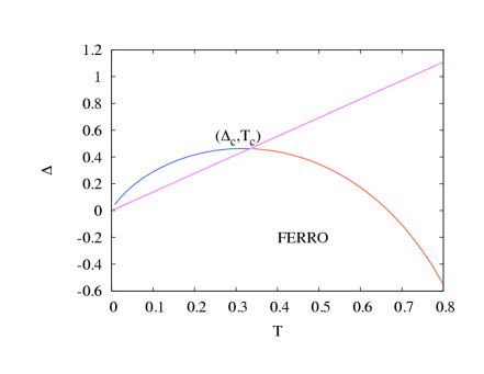
A quick inspection of equation 34 shows that the pure tri-critical point is not suppressed by disorder. Giving a disorder realization, $b(\beta)$ vanishes on the line $\beta\Delta=\ln 4$: the tri-critical point necessarily sits on this line. More precisely, its locus is given by:

$$(\Delta_{c}(N),T_{c}(N))=(\frac{2\ln 2}{3N}\sum_{i}\xi_{i}^{2},\frac{1}{3N}\sum_{i}\xi_{i}^{2})$$ (38)

In the thermodynamic limit this gives back the tri-critical point of the pure model: $\overline{T_{c}(N)}=T_{c}(\infty)\equiv T_{c}$. Other choices of normalization of the $l_{i}$’s would have alter the location of the tricritical point but not changed the following results on critical properties and FSS. In the thermodynamic limit (large $N$) $\frac{1}{N}\sum\xi_{i}^{2}$ is distributed with a Gaussian law of width $\sigma N^{-1/2}$, where $\sigma$ depends on $\delta$. This leads to fluctuations of $T_{c}$ of order $N^{-1/2}$ and, as a consequence, similar fluctuations of $\Delta_{c}$ because of the relation $\beta\Delta=\ln 4$. This model mimics the ROM case: the thermal fluctuation given by $\nu d_{u}$ are of order $N^{-2/3}$ (this can be checked both for the pure and the disorder model) the disorder fluctuations, given by the fluctuations of the tri-critical point, of order $N^{-1/2}$.

To study the tri-critical properties of this model, we focus on the line $\beta\Delta=\ln 4$. Writing $\beta=\beta_{c}(N)+{\lambda}/{N^{2/3}}$, that is $\lambda\propto N^{2/3}(T_{c}(N)-T)$, one obtains at leading order in N:

$$Z(\beta) = \sqrt{\frac{N\beta}{2\pi}}\int dm\ e^{-N\beta f(\beta)}$$

$$= \frac{\alpha\pi^{2}}{\beta_{c}(N)}\sqrt{\frac{\beta}{2}}\left(\frac{3}{2}\right)^{N}N^{1/3}\mathcal{F}\left(-\frac{\lambda\alpha}{\beta_{c}(N)^{2}}\right)\ ,$$

$$\mathcal{F}(x)=Ai^{2}(x)+Bi^{2}(x)\ \ \alpha=\frac{270}{8}\$$ , (39)

where, $Ai(x)$ and $Bi(x)$ are the well-known Airy functions. They are two linearly independent solutions of the equation: $y^{\prime\prime}-xy=0$. Their asymptotics, which would be useful to obtain the tails of the scaling functions of the different thermodynamic observables, is quite simple:

$$Ai^{2}(x)+Bi^{2}(x) \sim \frac{1}{\pi\sqrt{-x}}\ \ \ x\leq-1\ ,$$

$$Ai^{2}(x)+Bi^{2}(x) \sim \frac{e^{\frac{4}{3}x^{3/2}}}{4\pi x^{1/2}}\ \ \ x\geq 1\ .$$ (40)

As a consequence for a given disorder realization, the partition function has a standard finite-size scaling form like for equation 21, and that $\mathcal{F}$ is independent of the realization of the disorder.

As sketched in subsection 5.2, averaging on the disorder is here strictly equivalent to average on the distribution of tri-critical temperatures:

$$p(T_{c}(N)) = \sqrt{\frac{N}{2\pi\sigma^{2}}}e^{-N\frac{(T_{c}(N)-T_{c})^{2}}{2\sigma^{2}}}$$ (41)

For instance, let us detail the computation of the fluctuations of the order parameter $m$ defined as:

$$m=\frac{1}{N}\sum\xi_{i}S_{i}$$ (42)

Using the definition of $<m>$, one gets for a given disorder realization:

$$<m> = N^{-1/6}\frac{1}{\beta_{c}(N)}f\left(-\frac{\lambda}{\beta_{c}(N)^{2}}\right)+\mathcal{O}(N^{-5/6})$$

with,

$$f(x)=\frac{51840^{1/3}\pi Bi(\alpha x)+\frac{45x^{2}}{2}\ {{}_{2}F_{1}}(1;4/3,5/3;15x^{3})}{\alpha\pi^{3/2}\left(Ai^{2}(x\alpha)+Bi^{2}(x\alpha)\right)}$$

And in a more transparent form:

$$(T>T_{c}(N)) f(x>1)\propto e^{-cst\ x^{3/2}}x^{1/4}$$

$$(T<T_{c}(N)) f(x<-1)\propto(-x)^{1/4}$$

As expected, the tail exponent of the scaling function are those one would have find if one had computed the magnetization by steepest descent. One see clearly, that the magnetization plays in this model the same role as the dynamical overlap.

Similarly, one can compute the non-connected fluctuations of the order parameter,

$$N<m^{2}>=N^{2/3}\frac{1}{\beta_{c}(N)^{2}}g(-\frac{\lambda}{{\beta_{c}(N)^{2}}})+\mathcal{O}(1)$$

where

$$g(x) = \left((2160)^{1/3}\frac{Ai^{\prime}(x\alpha)Ai(x\alpha)+Bi^{\prime}(x\alpha)Bi(x\alpha)}{Ai^{2}(x\alpha)+Bi^{2}(x\alpha)}\right)$$

Again the asymptotics of g gives back the thermodynamic exponents.

$$(T>T_{c}(N)) g(x>1)\propto\frac{1}{x}$$

$$(T<T_{c}(N)) g(x<-1)\propto\sqrt{x}$$

The non-connected fluctuations have the same behavior as $\chi_{4}$ for the ROM.

Figure 19: Scaling-function of $N<\delta m^{2}>$, on this plot $x>0$ corresponds to $T>T_{c}$

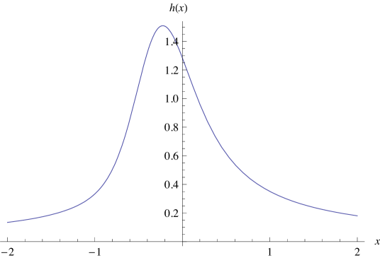
To finish this exercise the connected susceptibility is given by, see figure 19:

$$N<\delta m^{2}> = N^{2/3}h\left(-\frac{\lambda}{{\beta_{c}(N)^{2}}}\right)$$

$$h(|x|>1) \propto \frac{1}{x}$$

Now, we have to perform the average over the disorder. For this purpose, let us introduce $x=\sqrt{N}\frac{T_{c}(N)-T_{c}}{\sigma}$. One has:

$$\overline{\mathcal{O}}(T) = \frac{N^{2a/3}}{\sqrt{2\pi}}\int dxe^{-\frac{x^{2}}{2}}\mathcal{F}(N^{2/3}(\epsilon)+N^{1/6}x)$$ (43)

As showed in the previous appendix, this integral has two parts: a regular part, corresponding to the small value of $x$, and a singular part given by the tails of $\mathcal{F}(x)\sim x^{-a}$ for $x>>1$.

To compute this part, one has to consider all the contributions coming from the temperature range: $|T-T_{c}(N)|>cN^{-2/3}$ i.e. such that $\sigma x>-N^{1/2}(T-T_{c})+cN^{-1/6}$. By defining $\sigma x_{0}\equiv N^{1/2}(T-T_{c})$, one gets:

$$\overline{\mathcal{O}}(T) \simeq \frac{N^{a/2}}{\sqrt{2\pi}}\int_{\sigma(x+x_{0})>cN^{-1/6}}\frac{e^{-\frac{x^{2}}{2}}}{(x_{0}+x)^{a}}$$ (44)

We are now exactly in the same framework as discussed in section 5.2. These simple examples show how the analysis of this toy model is instructive. It is a fully solvable example of a weak-disordered model, for $\delta\neq 0$, with an exponent $\nu=1/2$ and an upper dimension $d_{u}=3$, that is $\nu d_{u}=3/2$ [70] where FSS is not the standard one. It gives also a clear insight in understanding the competition of the thermal and disorder fluctuations.

References

- [1] Das S P 2004 Rev. Mod. Phys. 76 785
- [2] Götze W 2009 Complex Dynamics of Glass Forming Liquids (Oxford University Press)
- [3] Kirkpatrick T and Wolynes P 1987 Phys. Rev. B 36 8552
- [4] Kirkpatrick T, Thirumalai D and Wolynes P 1989 Phys. Rev. A 40 1045
- [5] Kirkpatrick T and Wolynes P 1987 Phys. Rev. B 35 3072
- [6] Bouchaud J P, Cugliandolo F, Kurchan J and Mézard M 1996 Physica A 226 243
- [7] Cavagna A 2009 To appear in Phys. Rep., cond–mat arXiv:0903.4264
- [8] Lubchenko V and Wolynes P G 2007 Annu. Rev. Phys. Chem. 58 235
- [9] Andreanov A, Biroli G and Bouchaud J P 2009 cond-mat arXiv:0903.4619
- [10] Biroli G and Bouchaud J P 2004 Europhys. Lett. 67 21–27
- [11] Biroli G, Bouchaud J P, Miyazaki K and Reichman D R 2006 Phys. Rev. Lett. 97 195701
- [12] Franz S and Parisi G 2000 J. Phys. Condens. Matter 12 6335
- [13] Biroli G and Bouchaud J P 2007 J. Phys. C 19 205101
- [14] Berthier L, Biroli G, Bouchaud J P, Kob W, Miyazaki K and Reichman D 2007 J. Chem. Phys. 126 184503
- [15] Karmakar A, Dasgupta D and Sastry S 2009 PNAS 106 3675
- [16] Marinari E and Parisi G 1992 Europhys. Lett. 19 451–459
- [17] Billoire A, Giomi L and Marinari E 2005 Europhys. Lett. 71 824
- [18] Marinari E, Parisi G and Ritort F 1994 J. Phys.A: Math.Gen. 27 7647
- [19] Parisi G and Potters M 1995 J. Phys. A 28 5267
- [20] Brangian C, Kob W and Binder K 2002 J.Phys. A: Math Gen 35 191
- [21] Brangian C, Kob W and Binder K 2002 Phil. Mag. B 82 663
- [22] Brangian C, Kob W and Binder K 2001 Europhys. Lett. 53 756
- [23] Brangian C 2003 Physica A 338 471–478.
- [24] Crisanti A and Ritort F 2002 J.Phys: Condens. Matter 14 1381
- [25] Crisanti A and Ritort F 2000 Physica A 280 155
- [26] Cherrier R, Dean D and Lefèvre A 2003 Phys. Rev. E 67 046112
- [27] Krakoviack V and Alba-Simionesco C 2002 J. Chem. Phys. 117 2161
- [28] Cugliandolo F 2004 Slow Relaxations and nonequilibrium dynamics in condensed matter (Les Houches Summer School vol LXXVII) (Springer Berlin / Heidelberg) chap 7: Dynamics of Glassy Systems, pp 367–521
- [29] Castellani T and Cavagna A 2005 J. Stat. Mech. P05012
- [30] Thouless D, Anderson P and Palmer R 1987 Phil. Mag. A 35 593
- [31] Kurchan J and Laloux L 1996 J.Phys. A: Math Gen 29 1929–1948
- [32] Götze W and Sjögren L 1992 Rep. Prog. Phys. 55 241
- [33] Reichman D and Charbonneau P 2005 J. Stat. Mech. P05013
- [34] Götze W 1991 Liquids, Freezing and the Glass Transition (Les Houches Summer School vol LI) (North-Holland / Amsterdam) p 287
- [35] Ediger M D 2000 Annual Review of Physical Chemistry 51 99–128
- [36] Dasgupta C, Indrani A, Ramaswami S and Phani M 1991 Europhysica Letter 15 307
- [37] Franz S, Donati C, Parisi G and Glotzer S 1999 Phil. Mag. B 79 1827–1831
- [38] Toninelli C, Wyart M, Berthier L, Biroli G and Bouchaud J P 2005 Phys. Rev. E 71 041505
- [39] Franz S and Montanari A 2007 J. Phys. A 40 F251
- [40] Tesi M C, Rensburg E J V, Orlandini E and Whittington G 1996 J. Stat. Phys 82 155
- [41] Hukusima K and Nemoto K 1996 J. Phys. Soc. Japan 65 1604–1608
- [42] Lyubartsev A, Martsinovski A and Shevkanov S 1992 J. Chem. Phys. 96 1776–1783
- [43] Jacobs L and Rebbi C 1981 Journal of Computational Physics 41 203
- [44] Santen L and Krauth W 2000 Nature 405 550
- [45] Billoire A and Marinari E 2002 Europhys. Lett. 60 775–781
- [46] Parisi G and Potters M 1995 J. Phys.A: Math.Gen. 28 5267
- [47] Bernasconi J 1987 J. Phys. France 48 559
- [48] Bouchaud J P and Mézard M 1994 J. Phys. I (France) 4 1109
- [49] Picco M, Ritort F and Sales M 2001 The European physical journal. B 19 565–582
- [50] Marinari E, Naitza C, Parisi G, Picco M, Ritort F and Zuliani F 1999 Phys. Rev. Lett. 82 5175
- [51] Leutheusser E 1984 Phys. Rev. A 29 2765–2773
- [52] Fuchs M, Götze W, Hofacker I and Latz A 1991 J. Phys. Condens. Matter 3 5047
- [53] Kim B and Latz A 2001 Europhys. Lett. 53 660
- [54] Brézin E 1982 J.Phys (Paris) 43 15
- [55] Brézin E and Zinn-Justin J 1985 Nuclear Phys. B 257 867–893
- [56] Binder K, Nauenberg M, Privman V and Young A P 1985 Phys. Rev. B 31 1498–1502
- [57] Harris A 1974 J. Phys. C 7 1671
- [58] Chayes J T, Chayes L, Fisher D S and Spencer T 1986 Phys. Rev. Lett. 57 2999–3002
- [59] Aharony A and Harris A B 1996 Phys. Rev. Lett. 77 3700–3703
- [60] Wiseman S and Domany E 1998 Phys. Rev. E 58 2938–2951
- [61] Monthus C and Garel T 2007 Markov Processes and Related Fields 13 731–760
- [62] Fisher D S 1995 Phys. Rev. B 51 6411
- [63] Ioffe L B and Sherrington D 1998 Phys. Rev. B 57 7666
- [64] Lopatin A V and Ioffe L 2000 Phys. Rev. Lett. 84 4208
- [65] Lopatin A V and Ioffe L 1999 Phys. Rev. B 60 6412
- [66] Berthier L, Biroli G, Bouchaud J P, Kob W, Miyazaki K and Reichman D 2007 J. Chem. Phys. 126 184504
- [67] Berthier L 2003 Phis. Rev. Lett. 91 055701
- [68] Cardy J L 1988 Finite-Size Scaling (Elsevier Science Ltd)
- [69] Jones J L and Young A P 2005 Phys. Rev. B 71 174438
- [70] Blume M, Emery V J and Griffiths R B 1971 Phys. Rev. A 4 1071–1077