Volatility derivatives in market models with jumps

Abstract.

It is well documented that a model for the underlying asset price process that seeks to capture the behaviour of the market prices of vanilla options needs to exhibit both diffusion and jump features. In this paper we assume that the asset price process $S$ is Markov with càdlàg paths and propose a scheme for computing the law of the realized variance of the log returns accrued while the asset was trading in a prespecified corridor. We thus obtain an algorithm for pricing and hedging volatility derivatives and derivatives on the corridor-realized variance in such a market. The class of models under consideration is large, as it encompasses jump-diffusion and Lévy processes. We prove the weak convergence of the scheme and describe in detail the implementation of the algorithm in the characteristic cases where $S$ is a CEV process (continuous trajectories), a variance gamma process (jumps with independent increments) or an infinite activity jump-diffusion (discontinuous trajectories with dependent increments).

1. Introduction

Derivative securities on the realized variance of the log returns of an underlying asset price process trade actively in the financial markets. Such derivatives play an important role in risk management and are also used for expressing a view on the future behaviour of volatility in the underlying market. Since the liquid contracts have both linear (variance swaps) and non-linear (square-root = volatility swaps, hockey stick = variance options) payoffs, it is very important to have a robust algorithm for computing the entire law of the realized variance. Often such contingent claims have an additional feature, which makes them cheaper and hence more attractive to the investor, that stipulates that variance of log returns accrues only when the spot price is trading in a contract-defined corridor (see Subsection 2.1 for the precise definitions of such derivatives).

It is clear from these definitions that, in order to manage the risks that arise in the context of volatility derivatives, one needs to apply the same modelling framework that is being used for pricing and hedging vanilla options on the underlying asset. It has therefore been argued that the pricing and hedging of volatility derivatives should be done using models with jumps and stochastic volatility (see for example [10], Chapter 11). In this paper we propose a scheme for computing the distribution of the realized variance and the corridor-realized variance when the underlying process $S=(S)_{t\geq 0}$ is a Markov process with possibly discontinuous trajectories, thus obtaining an algorithm for pricing and hedging all the payoffs mentioned above. Our main assumption is that the Markov dimension of $S$ is equal to one (i.e. we assume that the future and past of the process $S$ are independent given its present value). We do not make any additional assumptions on the structure of the increments or the distributional properties of the process $S$. This class of processes is large as it encompasses one dimensional jump-diffusions and Lévy processes.

The algorithm consists of two steps. In the first step the original Markov process $S$ under a risk-neutral measure is approximated by a continuous-time finite state Markov chain $X=(X_{t})_{t\geq 0}$. This is achieved by approximating the generator of $S$ by a generator matrix for $X$. The second step consists of pricing the corresponding volatility derivative in the approximate model $X$. It should be stressed that the two steps are independent of each other but both clearly contribute to the accuracy of the scheme. In other words the second step can be carried out for any approximate generator matrix of the chain $X$. In specific examples in this paper we describe a natural way of defining the approximate generator matrix (see Section 4 for diffusions and Section 5 for processes with jumps) which is by no means optimal (see monograph [9] for weak convergence of such approximations and [16] for possible improvements) but already makes the proposed scheme accurate enough (see the numerical results in Section 6).

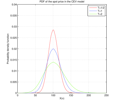
(a) The probability distribution function for the spot price $X_{T}$, with the maturity $T$ equal to 0.5, 1 and 2 years, where $X$ is the Markov chain used to approximate the CEV process $S$. For a precise description of the process $X$ see Subsection 6.1. All relevant parameter values are given in the caption of Table 2.

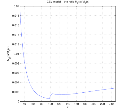
(b) The function $x\mapsto M_{2}(x)/M_{1}(x)$, where $x\in E$, in the CEV model. The minimum of this function, which equals $0.000563$, determines the value of the spacing $\alpha$ by the second inequality in (33). The maximum of the ratio, which is $0.019$, determines the largest jump-size multiple $n$ by the first inequality in (33). All relevant parameter values for the CEV model and the accompanying chain $X$ are given in the caption of Table 2.

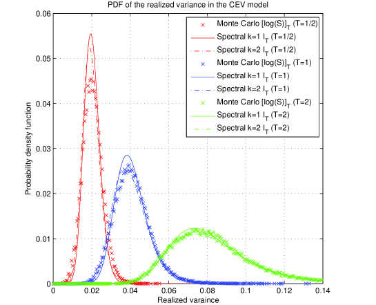
(c) The empirical probability distribution of the realized variance $[\log(S)]_{T}$ of the CEV model $S$, based on the Monte Carlo simulation described in Subsection 6.2, and the distribution of the random variable $I_{T}$, obtained from Theorem 2.1, for $T\in\{0.5,1,2\}$. For details on the definition of $I_{T}$ see Sections 2 and 4. Note that the computational time required to obtain the law of $I_{T}$ is independent of $T$ (see caption of Table 5).

Figure 1. CEV model

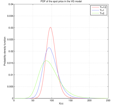
(a) The probability distribution function for the spot price $X_{T}$, with the maturity $T$ equal to 0.5, 1 and 2 years, where $X$ is the Markov chain used to approximate the variance gamma process. For a precise description of the process $X$ see Subsection 6.1. All relevant parameter values are given in the caption of Table 3.

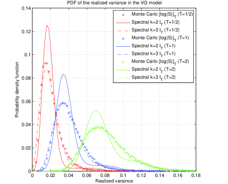
(b) The empirical probability distribution of the realized variance $[\log(S)]_{T}$ in the VG model $S$, based on the Monte Carlo simulation described in Subsection 6.3, and the distribution of the random variable $I_{T}$ for $T\in\{0.5,1,2\}$ matching $k\in\{2,3\}$ instantaneous moments. For details on $I_{T}$ see Sections 2 and 5. Note that the computational time required to obtain the law of $I_{T}$ is independent of $T$ and that the quality of the approximation is greater for $k=3$ (see also Table 6).

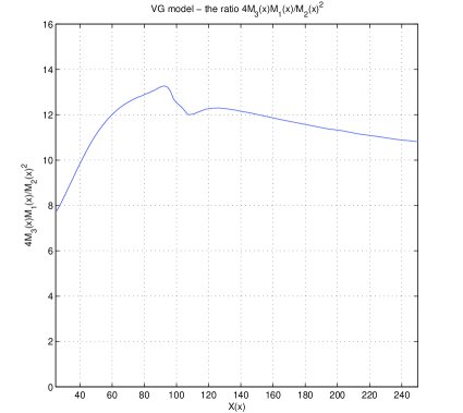
(c) The function $x\mapsto\frac{4M_{1}(x)M_{3}(x)}{M_{2}(x)^{2}}$, for $x\in E$ such that $20\leq x\leq 250$, in the variance gamma model. This function appears in condition (42) of Subsection 5.2. The parameters of the chain $X$ are given in the caption of Table 3.

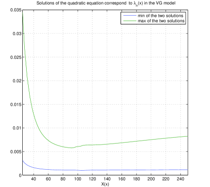
(d) The functions $x\mapsto\underline{\alpha}(x)$ and $x\mapsto\overline{\alpha}(x)$, for $x\in E$ such that $20\leq x\leq 250$, are the zeros of the quadratic in condition (40) in the variance gamma model. As summarised in Table 1, in order to ensure that the intensity $\lambda_{n}(x)$ is positive, we must choose the value of the constant $\alpha$ to lie between the two curves for all $x$ in the above range (see also Subsection 6.3).

Figure 2. Variance gamma model

In the second step of the algorithm we approximate the dynamics of the corridor-realized variance of the logarithm of the chain $X$ (i.e. the variance that accrued while $X$ was in the prespecified corridor) by a Poisson process with an intensity that is a function of the current state of the chain $X$. This approximation is obtained by matching $k\in\mathbb{N}$ instantaneous conditional moments of the corridor-realized variance of the chain $X$. This is a generalisation of the method proposed in [1], which in the framework of this paper corresponds to $k=1$ and only works in the case of linear payoffs on the realized variance (i.e. variance swaps) as can be seen in Tables 5, 6 and 7 of Section 6. Using $k$ strictly larger than one improves considerably the quality of the approximation to the distribution of the corridor-realized variance for $S$. In fact if $S$ is a diffusion process, then our algorithm with $k=2$ produces prices for the non-linear volatility payoffs (e.g. volatility swaps and options on variance) which are within a few basis points of the true price (see Table 5 and Figure 1c). If the trajectories of $S$ are discontinuous, then the scheme with $k=3$ appears to suffice (see Tables 6 and 7 and Figures 2b and 3a). Note also that in [14] we provide a straightforward implementation of our algorithm in Matlab for $k=3$. Furthermore in Section 3 we prove the weak convergence of our scheme as $k$ tends to infinity (see Theorem 3.1).

The general approach of this paper is to view continuous-time Markov chains as a numerical tool that is based on probabilistic principles and can therefore be applied in a very natural way to problems in pricing theory. It is worth noting that there is no theoretical obstruction for extending our scheme to the case when $S$ is just one component of a two dimensional Markov process (e.g. $S$ is the asset price in a stochastic volatility model) by using a Markov chain to approximate this two dimensional process. The reason why throughout this paper we assume that $S$ itself is Markov lies in the feasibility of the associated numerical scheme. If $S$ is Markov the dimension of the generator of $X$ can be as small as $70$, while in the case of the stochastic volatility process we would need to find the spectra of matrices of dimension larger than $2000$. This is by no means impossible but is not the focus of the present paper.

The literature on the pricing and hedging of derivatives on the realized variance is vast. It is generally agreed that either the assumption on the independence of increments or the continuity of trajectories of the underlying process needs to be relaxed in order to obtain a realistic model for the realized variance. In the recent paper [3] model independent bounds for options on variance are obtained in a general continuous semimartingale market. The continuity assumption is relaxed in [7], where a class of one dimensional Markov processes with independent increments is considered and the law of the realized variance is obtained. A perfect replication for a corridor variance swap (i.e. the mean of the corridor-realized variance) in the case of a continuous asset price process is given in [6]. For other contributions to the theory of volatility derivatives see [1] and the references therein. The main aim of this paper is to provide a stochastic approximation scheme for the pricing and hedging of derivatives on the realized (and corridor-realized) variance in models that violate both the above assumptions, thus making it virtually impossible to find the laws of the relevant random variables in semi-analytic form.

The paper is organised as follows. Section 2 defines the approximating Markov chains and gives a general description of the pricing algorithm. In Section 3 we state and prove the weak convergence of the proposed scheme. Section 5 (resp. 4) describes the implementation of the algorithm in the case where the process $S$ is an infinite activity jump-diffusion (resp. has continuous trajectories). Section 6 contains numerical results and Section 7 concludes the paper.

2. The $k$ conditional moments of the realized variance

Let $S=(S_{t})_{t\geq 0}$ be a strictly positive Markov process with càdlàg paths (i.e. each path is right-continuous as a function of time and has a left limit at every time $t$) which serves as a model for the evolution of the risky security under a risk-neutral measure. Note that we are also implicitly assuming that $S$ is a semimartingale.

2.1. The contracts

A volatility derivative in this market is any security that pays $\phi([\log(S)]_{T})$ at maturity $T$, where $\phi:\mathbb{R}_{+}\to\mathbb{R}$ is a measurable payoff function and $[\log(S)]_{T}$ is the is the quadratic variation of the process $\log(S)=(\log(S_{t}))_{t\geq 0}$ at maturity $T$ defined by

(1) $$[\log(S)]_{T} := \lim_{n\to\infty}\sum_{t_{i}^{n}\in\Pi_{n},i\geq 1}\left(\log\frac{S_{t_{i}^{n}}}{S_{t^{n}_{i-1}}}\right)^{2},$$

where $\Pi_{n}=\{t_{0}^{n},t_{1}^{n},\ldots,t_{n}^{n}\}$, $n\in\mathbb{N}$, is a refining sequence of partitions of the interval $[0,T]$. In other words $t_{0}^{n}=0$, $t_{n}^{n}=T$, $\Pi_{n}\subset\Pi_{n+1}$ for all $n\in\mathbb{N}$ and $\lim_{n\to\infty}\max\{|t_{i}^{n}-t_{i-1}^{n}|:i=1,\ldots,n\}=0$. It is well-known that this sequence converges in probability (see [13], Theorem 4.47). Many such derivative products trade actively in financial markets across asset-classes (see [1] and the references therein).

A corridor variance swap is a derivative security with a linear payoff function that depends on the accrued variance of the asset price $S$ while it is trading in an interval $[L,U]$ that is specified in the contract, where $0\leq L<U\leq\infty$. More specifically if we define a process

(2) $$\overline{S}_{t}:=\max\{L,\min\{S_{t},U\}\},\qquad\forall t\in[0,\infty),$$

then for a given partition $\Pi_{n}=\{t_{0}^{n},t_{1}^{n},\ldots,t_{n}^{n}\}$ of the time interval $[0,T]$ the corridor-realized variance is given by

(3) $$\sum_{t_{i}^{n}\in\Pi_{n},i\geq 1}\left[\mathbf{1}_{[L,U]}(S_{t^{n}_{i-1}})+\mathbf{1}_{[L,U]}(S_{t^{n}_{i}})-\mathbf{1}_{[L,U]}(S_{t^{n}_{i-1}})\mathbf{1}_{[L,U]}(S_{t^{n}_{i}})\right]\left(\log\frac{\overline{S}_{t_{i}^{n}}}{\overline{S}_{t^{n}_{i-1}}}\right)^{2},$$

where $\mathbf{1}_{[L,U]}$ denotes the indicator function of the interval $[L,U]$. In practice the increments $t^{n}_{i}-t^{n}_{i-1}$ ususally equal one day. The square bracket in the sum in (3) ensures that the accrued variance is not increased when the asset price $S$ jumps over the interval $[L,U]$.

The one sided corridor-realized variance was defined in [4]. Definition (1.1) in [4] (resp. (1.2) in [4]) corresponds to expression (3) above if we choose $U=\infty$ (resp. $L=0$). Formulae (1.1) and (1.2) in [4] are used to define the corridor-realized variance in a way which treats the entrance of $S$ into the corridor differently from its exit from the corridor. This asymmetry is then exploited to obtain an approximate hedging strategy for linear payoffs on the corridor-realized variance. In this paper we opt for a symmetric treatment of the entrance and exit of $S$ into and from the corridor $[L,U]$, because this is in some sense more natural. It is however important to note that all the theorems and the algorithm proposed here do NOT depend in any significant way on this choice of definition. In other words for any reasonable modification of the definition in (3) (e.g. the one in [4]) the algorithm described in this section would still work. Note also that our algorithm will yield an approximate distribution of random variable (3) in the model $S$ and therefore allows us to price any non-linear payoff that depends on the corridor-realized variance.

In the case the corridor-realized variance is monitored continuously (see [6]), we can express it using quadratic variation as follows. Note first that since the map $s\mapsto\max\{L,\min\{s,U\}\}$ can be expressed as a difference of two convex functions, Theorem 66 in [18] implies that the process $\overline{S}=(\overline{S}_{t})_{t\geq 0}$ is again a semimartingale and therefore the corridor-realized variance $Q^{L,U}_{T}(S)$, defined as the limit of the expression in (3) as $n$ tends to infinity, exists and equals

(4) $$Q^{L,U}_{T}(S) = [\log(\overline{S})]_{T}-\left(\log\frac{U}{L}\right)^{2}\sum_{0\leq t\leq T}\left[\mathbf{1}_{(0,L)}(S_{t-})\mathbf{1}_{(U,\infty)}(S_{t})+\mathbf{1}_{(0,L)}(S_{t})\mathbf{1}_{(U,\infty)}(S_{t-})\right]$$

by Theorem 4.47a in [13]. Since we are assuming that the process $S$ is càdlàg the limit $S_{t-}:=\lim_{s\nearrow t}S_{s}$ exists almost surely for all $t>0$. The sum in (4), which corresponds to jumps of the asset price $S$ over the corridor $[L,U]$, is almost surely finite by Theorem 4.47c in [13]. Note also that if $L=0$ (resp. $U=\infty$) we find that $Q^{0,U}_{T}(S)$ (resp. $Q^{L,\infty}_{T}(S)$) equals the quadratic variation of the semimartingale $\log(\overline{S})=(\log(\overline{S}_{t}))_{t\geq 0}$ because the process $S$ cannot in these cases jump over the corridor. Our main task it to find an approximate law of the random variable $Q^{L,U}_{T}(S)$ which will allow us to price any derivative on the corridor-realized variance with terminal value $\phi(Q^{L,U}_{T}(S))$, where $\phi$ is a possibly non-linear function.

2.2. Markov chain $X$ and its corridor-realized variance

Let us start by assuming that we are given a generator matrix $\mathcal{L}$ of a continuous-time Markov chain $X=(X_{t})_{t\geq 0}$ which approximates the generator of the Markov process $S$. The state-space of the Markov chain $X$ is the set $E:=\{x_{0},\ldots,x_{N-1}\}\subset\mathbb{R}_{+}$ with $N\in\mathbb{N}$ elements, such that $x_{i}<x_{j}$ for any integers $0\leq i<j\leq N-1.$ In Sections 4 and 5 we discuss briefly how to construct such approximate generators for Markov processes that are widely used in finance (i.e. diffusion processes with jumps.) Throughout the paper we will use the notation $\mathcal{L}(x,y)=e_{x}^{\prime}\mathcal{L}e_{y}$ for the elemetns of the matrix $\mathcal{L}$, where $x,y\in E$, vectors $e_{x},e_{y}$ denote the corresponding standard basis vectors of $\mathbb{R}^{N}$ and ^′ is transposition.

The quantities of interest are the quadratic variation $[\log(X)]=([\log(X)]_{t})_{t\geq 0}$ and the corridor-realized vaiance $Q^{L,U}(X)=(Q^{L,U}_{t}(X))_{t\geq 0}$ processes which are for any maturity $T$ defined by

(5) $$[\log(X)]_{T}:=\lim_{n\to\infty}\sum_{t_{i}^{n}\in\Pi_{n},i\geq 1}\left(\log\frac{X_{t_{i}^{n}}}{X_{t^{n}_{i-1}}}\right)^{2},$$

(6) $$Q^{L,U}_{T}(X):=[\log(\overline{X})]_{T}-\left(\log\frac{U}{L}\right)^{2}\sum_{0\leq t\leq T}\left[\mathbf{1}_{(0,L)}(X_{t-})\mathbf{1}_{(U,\infty)}(X_{t})+\mathbf{1}_{(0,L)}(X_{t})\mathbf{1}_{(U,\infty)}(X_{t-})\right],$$

where partitions $\Pi_{n}$, $n\in\mathbb{N}$, of $[0,T]$ are as in (1), the process $\overline{X}=(\overline{X}_{t})_{t\geq 0}$ is defined analogously with (2) by $\overline{X}_{t}:=\max\{L,\min\{X_{t},U\}\}$ and $X_{t-}:=\lim_{s\nearrow t}X_{s}$ for any $t>0$. Note that if we choose $L<\min\{x\>:\>x\in E\}$ and $U>\max\{x\>:\>x\in E\}$, then the random variables in (5) and (6) coincide. We can therefore without loss of generality only consider the corridor-realized variance $Q^{L,U}_{T}(X)$.

Since the process $X$ is a finite-state Markov chain, the jumps of $X$ arrive with bounded intensity and it is therefore clear that the following must hold

(7) $$\mathbb{P}\left[Q^{L,U}_{t+\Delta t}(X)-Q^{L,U}_{t}(X)\neq\left(\log\frac{\overline{X}_{t+\Delta t}}{\overline{X}_{t}}\right)^{2}\Bigg{\lvert}\>X_{t}=x\right]=o(\Delta t)\quad\text{for all}\quad x\in[L,U]\cap E.$$

An analogous equality holds if $X_{t}$ is ountside of the corridor $[L,U]$. Recall also that by definition a function $f(\Delta t)$ is of the order $o(\Delta t)$ (usually denoted by $f(\Delta t)=o(\Delta t)$) if and only if $\lim_{\Delta t\searrow 0}f(\Delta t)/\Delta t=0$. Equality (7) implies that the $j$-th instantaneous conditional moment of the corridor-realized variance $Q^{L,U}(X)$ is given by

(8) $$M_{j}(x) := \lim_{\Delta t\to 0}\frac{1}{\Delta t}\mathbb{E}\left[\left(Q^{L,U}_{t+\Delta t}(X)-Q^{L,U}_{t}(X)\right)^{j}\Big{\lvert}X_{t}=x\right]$$

$$= \sum_{y\in E}\mathcal{L}(x,y)\left[\left(\log\frac{\overline{y}}{\overline{x}}\right)^{2j}-\left(\log\frac{U}{L}\right)^{2j}\mathbf{1}_{A_{U,L}}(x,y)\right]$$

where the set $A_{U,L}\subset\mathbb{R}^{2}$ is defined as $A_{U,L}:=\left([0,L)\times(U,\infty)\right)\cup\left((U,\infty)\times[0,L)\right)$ and for any $x\in E$ we have $\overline{x}:=\max\{L,\min\{x,U\}\}$.

2.3. The extension $(X,I)$

The basic idea of this paper is to extend the markov chain $X$ to a continuous-time Markov chain $(X,I)=(X_{t},I_{t})_{t\geq 0}$ where the dynamics of the process $I$ approximates well the dynamics of the corridor-realized variance $Q^{L,U}(X)$. Conditional on the path of the chain $X$, the process $I$ will be a compound Poisson process with jump-intensity that is a function of the current state of $X$. The generator of $(X,I)$ will be chosen in such a way that the first $k\in\mathbb{N}$ infinitesimal moments of $I$ and $Q^{L,U}(X)$ coincide. The approximating chain $I$ will start at 0 (as does the process $Q^{L,U}(X)$) and gradually jump up its uniform state-space $\{0,\alpha,..,\alpha 2C\}$, where $\alpha$ is a small positive constant and $C$ is some fixed integer.

The main computational tool in this paper is the well-known spectral decomposition for partial-circulant matrices (see Appendices A.2-A.4 in [1] for the definition and the properties of the spectrum), which will be applied to the generator of the Markov chain $(X,I)$. The geometry of the state-space $\{0,\alpha,..,\alpha 2C\}$ is therefore of fundamental importance because it allows the generator of $(X,I)$ to be expressed as a partial-circulant matrix. As mentioned in the introduction, the main difference between the approach in the present paper and the algorithm in [1] is that here we take advantage of the full strength of the partial-circulant form of the generator of $(X,I)$. This allows us to define the process $I$ as a compound Poisson process with state-dependent intensity rather than just a Poisson process (which was the case in [1]), without adding computational complexity. As we shall see in Section 6 this enables us to approximate the entire distribution of the corridor-realized variance and hence obtian much more accurate numerical results.

Assuming that the process $I$ can jump at most $n\in\mathbb{N}$ states up from its current position in an infinitesimal amount of time, the dynamics of $I$ are uniquely determined by the state-dependent intensities

(9) $$\lambda_{i}:E\to\mathbb{R}_{+},\quad\text{ where }\quad i\in\{1,\ldots,n\}$$

and $E$ is the state-space of the chain $X$. The generator of $I$, conditional on the event $X_{t}=x$, can therefore for any $c,d\in\{0,1,..,2C\}$ be expressed as

(13) $$\mathcal{L}^{I}(x:c,d)\>:=\>\left\{\begin{array}[]{ll}\lambda_{j}(x)&\mathrm{if}\>\>d=c+j\!\!\!\mod(2C+1)\quad\text{for some}\quad j\in\{1,...,n\};\\ -\sum_{i=1}^{n}\lambda_{i}(x)&\mathrm{if}\>\>d=c;\\ 0&\text{ otherwise.}\end{array}\right.$$

The dimension of the matrix $\mathcal{L}^{I}(x:\cdot,\cdot)$ is $2C+1$ for all $x\in E$ and the identity $d=c+j\!\!\!\mod(2C+1)$ means that the numbers $d$ and $c+j$ represent the same element in the additive group $\mathbb{Z}_{2C+1}$. A key observation here is that the entries $\mathcal{L}^{I}(x:c,d)$ in the conditional generator depend on $c$ and $d$ solely through the difference $d-c$ and hence the afore mentioned group structure makes the conditional generator into a circulant matrix (see Appendix A for the definition of circulant matrices).

This algebraic structure of the conditional generator $\mathcal{L}^{I}(x:\cdot,\cdot)$ translates into a periodic boundary condition for the process $I$. This is very undesirable because the process $Q^{L,U}(X)$ we are trying to approximate clearly does not exhibit such features. We must therefore choose $C$ large enough so that even if the chain $I$ is allowed to jump $n$ steps up at any time, the probability that it oversteps the boundary is negligible (i.e. below machine precision). We will see in Section 6 that in practice $C\approx 100$ and $n\approx 30$ is sufficient to avoid the boundary. Since our aim is to match the first $k$ instantaneous moments, it is necessary to take $n$ larger or equal to $k$. In applications this does not pose additional restrictions because, as we shall see in Section 6, $k=3$ produces the desired results for jump-diffusions and $k=2$ is already enough for continuous processes.

The conditional generators given in (13) can be used to specify the generator of the Markov chain $(X,I)$ on the state-space $E\times\{0,\alpha,\ldots,\alpha 2C\}$ as follows

(14) $${\mathcal{G}}(x,c;y,d):=\mathcal{L}(x,y)\delta_{c,d}+\mathcal{L}^{I}(x:c,d)\delta_{x,y},$$

where $x,y\in E$, $c,d\in\{0,1,\ldots,2C\}$ and $\delta_{\cdot,\cdot}$ denotes the Kronecker delta function. The matrix ${\mathcal{G}}$ is of the size $N(2C+1)$ and has partial-circulant form. In other words we can express ${\mathcal{G}}$ in terms of $N^{2}$ blocks where each block is a square matrix of the size $2C+1$ and the blocks that intersects the diagonal of ${\mathcal{G}}$ are equal to a sum of a circulant matrix and a scalar multiple of the identity matrix. All other blocks are scalar matrices. For the precise definition of partial-circulant matrices see Appendix A.

We can now compute, using (13) and (14), the $j$-th instantaneous conditional moment of the process $I$ as follows

(15) $$\lim_{\Delta t\rightarrow 0}\frac{1}{\Delta t}\mathbb{E}\left[(I_{t+\Delta t}-I_{t})^{j}\Bigl{\lvert}X_{t}=x,I_{t}=\alpha c\right] = \sum_{d=0}^{2C}(\alpha d-\alpha c)^{j}\mathcal{L}^{I}(x:c,d)$$

$$= \alpha^{j}\sum_{d=1}^{n}d^{j}\lambda_{d}(x)$$

for any $x\in E$ and all integers $c\in\{0,1,\ldots,2C\}$ that satisfy the inequality $c<2C-n$, where $n$ was introduced in (9). This inequality implies that the process $I$ cannot jump to or above $\alpha 2C$ (i.e. it cannot complete a full circle) in a very short time interval $\Delta t$. Note also that it is through this inequality only that identity (15) depends on the current level $\alpha c$ of the process $I$.

Our main goal is to approximate the process $(X,Q^{L,U}(X))$, where corridor-realized variance $Q^{L,U}(X)$ is defined in (6), by the continuous-time Markov chain $(X,I)$ with generator given by (14). We now match the first $k$ instantaneous conditional moments of processes $Q^{L,U}(X)$ and $I$ using identities (8) and (15):

(16) $$\alpha^{j}\sum_{d=1}^{n}d^{j}\lambda_{d}(x)=M_{j}(x)\quad\text{for any}\quad x\in E\quad\text{and}\quad j=1,\ldots,k.$$

In other words we must choose the intensity functions $\lambda_{i}$ (see (9)) and the parameter $\alpha$ so that the system (16) is satisfied. The necessary requirement for the solution is that $\lambda_{i}(x)\geq 0$ for all $x\in E$ and all $i=1,\ldots,n$. These inequalities can place non-trivial restrictions on the solution space and will be analysed in more detail in Sections 4 and 5.

Another simple yet important observation that follows from (16) is that, in order to match the first $k$ instantaneous conditional moments of the corridor-realized variance $Q^{L,U}(X)$, the size of the support of the jump distribution of the of Poisson processes with state-dependant intensity (i.e. $n$) must be at least $k$. From now on we assume that $n\geq k$.

The pricing of volatility derivatives is done using the following theorem which yields a closed-form formula for the semingroup of the Markov chain $(X,I)$.

Theorem 2.1.

Let ${\mathcal{G}}$ be the generator matrix of the Markov process $(X,I)$ given by (14). Then for any $t\geq 0$, $x,y\in E$ and $d\in\{0,\ldots,2C\}$ the equality holds

(17) $$\mathbb{P}\left(X_{t}=y,I_{t}=\alpha d\big{\lvert}X_{0}=x\right) = \exp(t{\mathcal{G}})(x,0;y,d)$$

$$= \frac{1}{2C+1}\sum_{j=0}^{2C}e^{\mathtt{i}p_{j}d}\exp(t\mathcal{L}_{j})(x,y),$$

where $\mathtt{i}=\sqrt{-1}$, the scalars $p_{j}$ and the complex matrices $\mathcal{L}_{j}$, for $j=0,\ldots,2C$, are given by

(18) $$\mathcal{L}_{j}(x,y) := \mathcal{L}(x,y)+\delta_{x,y}\sum_{i=1}^{n}\left(e^{-\mathtt{i}p_{j}i}-1\right)\lambda_{i}(x),$$

$$p_{j} := \frac{2\pi}{2C+1}j.$$

Theorem 2.1 is the main computational tool used in this paper which allows us to find in a semi-analytic form the semigroup of the chain $(X,I)$ (if $C\approx 100$ and $N=70$, the matrix ${\mathcal{G}}$ contains more than $10^{8}$ elements). For a straightforward implementation of the algorithm in Matlab see [14]. It is clear that Theorem 2.1 generalizes equation (6) in [1] and that this generalization involves exactly the same number of matrix operations as the algorithm in [1]. The only additional computations are the sums in (18).

The proof of Theorem 2.1 relies on the partial-circulant structure of the matrix ${\mathcal{G}}$ given in (14). The argument follows precisely the same lines as the one that proved Theorem 3.1 in [1] and will therefore not be given here (see Appendix A.5 in [1] for more details).

Since the dynamics of the process $(X,I)$ are assumed to be under a risk-neutral measure, the current value of any payoff that depends on the corridor-realized variance at fixed maturity can easily be obtained from the formulae in Theorem 2.1. Furthermore the same algorithm yields the risk sensitivities Delta and Gamma of any derivative on the corridor-realized variance, without adding computational complexity. This is because the output of our scheme is a vector of values of the derivative in question conditional on the process $X$ starting at each of the elements in its state-space. We should also note that forward-starting derivatives on the corridor-realized variance can be dealt with using the same algorithm because conditioning on the state of a Markov chain at a future time requires only a single additional matrix-vector multiplication. Explicit calculations are obvious and are omitted (see [1] for more details).

3. Convergence

In Section 2 we defined the Markov chain $(X,I^{k})$ via its generator (14) that in some sense approximates the process $(X,Q^{L,U}(X))$, where $Q^{L,U}(X)$ is the corridor-realized variance of $X$ defined in (6). Here $I^{k}$ denotes the process $I$ from Section 2 which satisfies the instantaneous conditional moment restrictions, given by (16), up to order $k$.

Notice that it follows directly from definition (6) that the process $(X,Q^{L,U}(X))$ is adapted to the natural filtration generated by the chain $X$ and that its components $X$ and $Q^{L,U}(X)$ can only jump simultaneously. On the other hand note that the form of the generator of the chain $(X,I^{k})$, given by (14), implies that the components $X$ and $I^{k}$ cannot both jump at the same time. It is also clear that the process $I^{k}$ is not adapted to the natural filtration of $X$. In this section our goal is to prove that, in spite of these differences, for any fixed time $T$ the sequence of random variables $(I^{k}_{T})_{k\in\mathbb{N}}$ converges in distribution to the random variable $Q^{L,U}_{T}(X)$. In fact we have the following theorem which states that, for any bounded European payoff, the price of the corresponding derivative on the corridor-realized variance in the approximate model $(X,I^{k})$ converges to the price of the same derivative in $(X,Q^{L,U}(X))$ as the number $k$ of matched instantaneous conditional moments tends to infinity.

Theorem 3.1.

Let $X$ be a continuous-time Markov chain with generator $\mathcal{L}$ as given in Section 2. For each $k\in\mathbb{N}$ define a real number

(19) $$\alpha_{k} := \frac{1}{k}\max\left\{\left(\log\frac{y}{x}\right)^{2}\>:\>x,y\in E\backslash\{0\}\right\},$$

assume that $n$ in (9) equals $k$ and that there exist functions $\lambda_{i}^{k}:E\to\mathbb{R}_{+},$ $i\in\{1,\ldots,k\}$, that solve the system of equations (16). Let the continuous-time Markov chain $(X,I^{k})$ be given by generator (14) where the integers $C_{k}$ in (13), which determine the size of the state-space of the process $I^{k}$, are chosen in such a way that $\lim_{k\to\infty}\alpha_{k}C_{k}=\infty$. Then for any fixed time $T>0$ the sequence of random variables $(I_{T}^{k})_{k\in\mathbb{N}}$ converges weakly to $Q^{L,U}_{T}(X)$. In other words for any bounded continuous function $f:\mathbb{R}\to\mathbb{R}$ we have

$$\lim_{k\to\infty}\mathbb{E}[f(I_{T}^{k})\lvert X_{0}]=\mathbb{E}[f(Q^{L,U}_{T}(X))\lvert X_{0}].$$

Before proving Theorem 3.1 we note that the assumption on the existence of non-negative solutions of the system in (16) is not stringent and can be satisfies for any chain $X$ by allowing $n$ in (9) to take values larger than $k$. The restriction $n=k$ in Theorem 3.1 is used because it simplifies the notation.

Proof. Throughout this proof we will use the notation $\Sigma_{t}:=Q^{L,U}_{t}(X)$ for any $t\in\mathbb{R}_{+}$. By the Lévy continuity theorem it is enough to prove that the equality holds

$$\lim_{k\to\infty}\mathbb{E}[\exp(\mathtt{i}uI_{T}^{k})]=\mathbb{E}[\exp(\mathtt{i}u\Sigma_{T})]\quad\text{for each}\quad u\in\mathbb{R}.$$

Let $\Delta t>0$ be a small positive number and note that, by conditioning on the $\sigma$-algebra generated by the process $X$ up to and including time $T-\Delta t$ and using the Markov property, we obtain the following representation

$$\mathbb{E}[\exp(\mathtt{i}u\Sigma_{T})] = \mathbb{E}\left[\exp(\mathtt{i}u\Sigma_{T-\Delta t})\mathbb{E}\left[\exp(\mathtt{i}u(\Sigma_{T}-\Sigma_{T-\Delta t}))\big{\lvert}X_{T-\Delta t}\right]\right]$$

$$= \mathbb{E}\left[e^{\mathtt{i}u\Sigma_{T-\Delta t}}\left(\sum_{j=0}^{k}\frac{(\mathtt{i}u)^{j}}{j!}\mathbb{E}\left[(\Sigma_{T}-\Sigma_{T-\Delta t})^{j}\big{\lvert}X_{T-\Delta t}\right]\right.\right.$$

$$\left.\left.+\sum_{j=k+1}^{\infty}\frac{(\mathtt{i}u)^{j}}{j!}\mathbb{E}\left[(\Sigma_{T}-\Sigma_{T-\Delta t})^{j}\big{\lvert}X_{T-\Delta t}\right]\right)\right]$$

$$= \mathbb{E}\left[e^{\mathtt{i}u\Sigma_{T-\Delta t}}\left(1+\Delta t\sum_{j=1}^{k}\frac{(\mathtt{i}u)^{j}}{j!}M_{j}(X_{T-\Delta t})\right.\right.$$

$$\left.\left.+\sum_{j=k+1}^{\infty}\frac{(\mathtt{i}u)^{j}}{j!}\mathbb{E}\left[(\Sigma_{T}-\Sigma_{T-\Delta t})^{j}\big{\lvert}X_{T-\Delta t}\right]\right)\right]+o(\Delta t),$$

where $M_{j}$ is defined in (8). By applying Markov property of $(X,I^{k})$, identity (15) and condition (16), which holds by assumption for all $j\in\{1,\ldots,k\}$, we obtain

$$\mathbb{E}[\exp(\mathtt{i}uI^{k}_{T})] = \mathbb{E}\left[e^{\mathtt{i}uI^{k}_{T-\Delta t}}\left(1+\Delta t\sum_{j=1}^{k}\frac{(\mathtt{i}u)^{j}}{j!}M_{j}(X_{T-\Delta t})\right.\right.$$

$$\left.\left.+\sum_{j=k+1}^{\infty}\frac{(\mathtt{i}u)^{j}}{j!}\mathbb{E}\left[(I^{k}_{T}-I^{k}_{T-\Delta t})^{j}\bigg{\lvert}X_{T-\Delta t},I^{k}_{T-\Delta t}\right]\right)\right]+o(\Delta t).$$

It follows from (8) that there exists a positive constant $G$ such that $\max\{M_{j}(x)\>:\>x\in E\}\leq G^{j}$ for all $j\in\mathbb{N}$. Therefore we find that for a constant $D:=\exp(uG)$ the following inequality holds on the entire probability space

(22) $$\bigg{\lvert}\sum_{j=1}^{k}\frac{(\mathtt{i}u)^{j}}{j!}M_{j}(X_{T-\Delta t})\bigg{\rvert}\leq D.$$

Note also that $D$ is independent of $k$ and $\Delta t$.

Definition (19) implies that $k\alpha_{k}$ is a positive constant, say $A$, for each $k\in\mathbb{N}$. If we introduce a positive constant $L:=\max\{-\mathcal{L}(x,x)\>:\>x\in E\}$, we obtain the following bound

(23) $$\mathbb{E}\left[(\Sigma_{T}-\Sigma_{T-\Delta t})^{j}\big{\lvert}X_{T-\Delta t}\right] \leq A^{j}L\Delta t+o(\Delta t)\quad\text{for each}\quad j\in\mathbb{N}$$

on the entire probability space. In order to find a similar bound for the process $I^{k}$ we first note that if follows from the linear equation (16) (for $j=1$) and definition (19) that the inequalities

$$\sum_{d=1}^{k}d\lambda_{d}^{k}(x)\leq kL\quad\text{for all}\quad k\in\mathbb{N},\>x\in E$$

must hold. Therefore (15) implies

(24) $$\mathbb{E}\left[(I^{k}_{T}-I^{k}_{T-\Delta t})^{j}\bigg{\lvert}X_{T-\Delta t},I^{k}_{T-\Delta t}\right] \leq A^{j}kL\Delta t+o(\Delta t)\quad\text{for any}\quad j\in\mathbb{N}$$

and any small time-step $\Delta t$. We can now combine the estimates in (3), (3), (22), (23) and (24) to obtain the key bound

$$\left\lvert\mathbb{E}[\exp(\mathtt{i}u\Sigma_{T})]-\mathbb{E}[\exp(\mathtt{i}uI^{k}_{T})]\right\rvert \leq \left\lvert\mathbb{E}[\exp(\mathtt{i}u\Sigma_{T-\Delta t})]-\mathbb{E}[\exp(\mathtt{i}uI^{k}_{T-\Delta t})]\right\rvert(1+\Delta tD)$$

$$+\>\>L(k+1)\Delta t\sum_{j=k+1}^{\infty}\frac{(Au)^{j}}{j!}+o(\Delta t).$$

The main idea of the proof of Theorem 3.1 is to iterate the bound in (3) $\frac{T}{\Delta t}$ times. This procedure yields the following estimates

$$\left\lvert\mathbb{E}[\exp(\mathtt{i}u\Sigma_{T})]-\mathbb{E}[\exp(\mathtt{i}uI^{k}_{T})]\right\rvert \leq D\Delta t(1+\Delta tD)^{(T/\Delta t)-1}+L(k+1)T\sum_{j=k+1}^{\infty}\frac{(Au)^{j}}{j!}+T\frac{o(\Delta t)}{\Delta t}.$$

Since the left-hand side of this inequality is independent of $\Delta t$, the inequality must hold in the limit as $\Delta t\searrow 0$. We therefore find

(26) $$\left\lvert\mathbb{E}[\exp(\mathtt{i}u\Sigma_{T})]-\mathbb{E}[\exp(\mathtt{i}uI^{k}_{T})]\right\rvert\leq L(k+1)T\sum_{j=k+1}^{\infty}\frac{(Au)^{j}}{j!}.$$

The right-hand side of inequality (26) clearly converges to zero as $k$ tends to infinity. This concludes the proof of the theorem.

$\Box$

Theorem 3.1 implies that the prices of the volatility derivatives in the Markov chain model $X$ can be approximated arbitrarily well using the method defined in Section 2. Our initial problem of approximating prices in the model based on a continuous-time Markov process $S$ is by Theorem 3.1 reduced to the question of the approximation of the law of $S$ by the law of $X$. This can be achieved by a judicious choice for the generator matrix of the chain $X$. Since this is not the central topic of this paper we will not investigate the question further in this generality (see [9] for numerous results on weak convergence of Markov processes). However in Sections 4 and 5 we are going to propose specific Markov chain approximations for diffusion and jump-diffusion processes respectively and study numerically the behaviour of the approximations for volatility derivatives in Section 6.

4. The realized variance of a diffusion process

Our task now is to apply the method described in Section 2 to approximate the dynamics of the corridor-realized variance of a diffusion processes. The first step is to approximate the diffusion process $S$ which solves the stochastic differential equation (SDE)

(27) $$\frac{dS_{t}}{S_{t}}=\gamma dt+\sigma\left(\frac{S_{t}}{S_{0}}\right)dW_{t},$$

with measurable volatility function $\sigma:\mathbb{R}_{+}\to\mathbb{R}_{+}$, using a continuous-time Markov chain $X$. A possible way of achieving this is to use a generator for the chain $X$ given by the following system of linear equations

$$\sum_{y\in E}\mathcal{L}(x,y) = 0,$$

(28) $$\sum_{y\in E}\mathcal{L}(x,y)(y-x) = \gamma x,$$

$$\sum_{y\in E}\mathcal{L}(x,y)(y-x)^{2} = \sigma\left(\frac{x}{X_{0}}\right)^{2}x^{2}$$

for each $x\in E$. In Appendix B we give an algorithm to define the state-space $E$ of the chain $X$. In Section 6 we provide a numerical comparison for vanilla option prices in the CEV model, i.e. in the case $\sigma(s):=\sigma_{0}s^{\beta-1}$, and in the corresponding Markov chain model given by the approximation above. Note that a Markov chain approximation $X$ of the diffusion $S$ is in the spirit of [2] and is by no means the only viable alternative. One could produce more accurate results by matching higher instantaneous moments of the two processes (see [16] for rates of convergence in some special cases).

If the solution of SDE (27) is used as a model for the risky security under a risk-neutral measure we have to stipulate that $\gamma=r$, where $r$ is the prevailing risk-free rate in the economy. Therefore by the first two equations in system (4) the vector in $\mathbb{R}^{N}$ with cooridnates equal to the elements in the set $E$ represents an eigenvector of the matrix $\mathcal{L}$ for the eigenvalue $\gamma$. Hence we find

(29) $$\mathbb{E}[X_{t}\lvert X_{0}=x]=e_{x}^{\prime}\exp(t\mathcal{L})\sum_{y\in E}ye_{y} = e^{t\gamma}x,\qquad\forall x\in E,$$

where $e_{x}$ denotes the standard basis vector in $\mathbb{R}^{N}$ that corresponds to the element $x\in E$ in the natural ordering and the operation ^′ denotes transposition. Therefore, under the condition $\gamma=r$, the market driven by the chain $X$ will also have a correct risk-neutral drift.

Once we define the chain $X$, the next task is to specify the process $I$ that approximates well the corridor-realized variance $Q^{L,U}(X)$ defined in (6). As we shall see in Section 6, matching the first two moments (i.e. the case $k=2$ in Section 2) is sufficient to approximate the corridor-realized variance dynamics of a diffusion processes. It is therefore necessary to take $n\geq 2$, where $n$ is the number of states the approximate variance process $I$ can jump up by at any given time (see (9)). To have flexibility we use $n$ much larger than 2, usually around 30. However in order to maintain the tractability of the solution of system (16) we make an additional assumption that the intensities $\lambda_{i}$ in (9), for $i=2,\ldots,n$, are all equal to a single intensity function $\lambda_{n}:E\to\mathbb{R}_{+}$. To simplify the notation we introduce the symbol

(30) $$b_{j}^{n,m} := \sum_{l=n+1}^{m}l^{j},\qquad\text{where}\quad j,n,m\in\mathbb{N}\quad\text{and}\quad m>n.$$

System (16) can in this case be solved explicitly as follows

(31) $$\lambda_{1}(x) = \frac{\alpha M_{1}(x)b_{2}^{1,n}-M_{2}(x)b_{1}^{1,n}}{\alpha^{2}(b_{2}^{1,n}-b_{1}^{1,n})},\quad\text{for any}\quad x\in E,$$

(32) $$\lambda_{n}(x) = \frac{M_{2}(x)-\alpha M_{1}(x)}{\alpha^{2}(b_{2}^{1,n}-b_{1}^{1,n})},\quad\text{for any}\quad x\in E,$$

where $M_{j}(x)$ is given in (8). Since the functions $\lambda_{1},\lambda_{n}$ are intensities, all the values they take must be non-negative. The formulae above imply that this is satisfied if and only if the following inequalities hold

(33) $$\alpha\frac{b_{2}^{1,n}}{b_{1}^{1,n}}\>\geq\>\frac{M_{2}(x)}{M_{1}(x)}\>\geq\>\alpha\qquad\text{for all}\quad x\in E.$$

It is clear that the function $x\mapsto M_{2}(x)/M_{1}(x)$, $x\in E$, depends on the definition of the chain $X$ both through the choice of the state-space $E$ and the choice of the generator $\mathcal{L}$. Figure 1b contains the plot of this function in the special case of the CEV model. Inequalities (33) are used to help us choose a feasible value for the parameter $\alpha$ which determines the geometry of the state-space of the process $I$. Note also that (33) implies that the larger the value of $n$ is, the less restricted we are in choosing $\alpha$. In Section 6 we will make these choices explicit for the CEV model.

The generator of the approximate corridor-realized variance $I$, conditional on the chain $X$ being at the level $x$, is in general given by Formula (13). In this particular case the non-zero matrix elements $\mathcal{L}^{I}(x:c,d)$, $c,d\in\{0,1,\ldots,2C\}$, are given by

$$\mathcal{L}^{I}(x:c,d) := \left\{\begin{array}[]{ll}\lambda_{1}(x)&\mathrm{if}\>\>d=(c+1)\!\!\!\mod(2C+1);\\ \lambda_{n}(x)&\mathrm{if}\>\>d=(c+i)\!\!\!\mod(2C+1),\>i\in\{2,...,n\};\\ -\lambda_{1}(x)-(n-1)\lambda_{n}(x)&\mathrm{if}\>\>d=c.\end{array}\right.$$

This defines explicitly (via equations (31) and (32)) the dynamics of the chain $(X,I)$ if the original asset price process $S$ is a diffusion. In Section 6 we will describe an implementation of this method when $S$ follows a CEV process and study the behaviour of certain volatility derivatives in this model.

5. The realized variance of a jump-diffusion

In this section the task is to describe the algorithm for the pricing of volatility derivatives in jump-diffusion models. This will be achieved by an application of the algorithm from Section 2 with $k=3$. In Section 6 we will investigate numerically the quality of this approximation. We start by describing a construction of the Markov chain which is used to approximate a jump-diffusion.

5.1. Markov chain approximations for jump-diffusions

We will consider a class of processes with jumps that is obtained by subordination of diffusions. The prototype for such processes is the well-known variance gamma model defined in [15], which can be expressed as a time-changed Brownian motion with drift.

A general way of building (possibly infinite-activity) jump-diffusion processes is by subordinating diffusions using a class of independent stochastic time changes. Such a time change is given by a non-decreasing stationary process $(T_{t})_{t\geq 0}$ with independent increments, which starts at zero, and is known as a subordinator. The law of $(T_{t})_{t\geq 0}$ is characterized by the Bernstein function $\phi(\lambda)$, defined by the following identity

(35) $$\mathbb{E}\left[\exp(-\lambda T_{t})\right]=\exp(-\phi(\lambda)t)\quad\text{for any}\quad t\geq 0\quad\text{and}\quad\lambda\in D,$$

where $D$ is an interval in $\mathbb{R}$ that contains the half-axis $[0,\infty)$. For example in the case of the variance gamma process, the Bernstein function is of the form

(36) $$\phi(\lambda)=\frac{\mu^{2}}{\nu}\log\left(1+\lambda\frac{\nu}{\mu}\right).$$

In this case $(T_{t})_{t\geq 0}$ is a gamma process with characteristic function equal to $\mathbb{E}[\exp(\mathtt{i}uT_{t})]=\exp(-\phi(-\mathtt{i}u)t)$. Note that the set $D$ in (35) is in this case equal to $(-\mu/\nu,\infty)$ (see [15], equation (2)). This subordinator is used to construct the jump-diffusions in Section 6.

Let $S$ be a diffusion defined by the SDE in (27). If we evaluate the process $S$ at an independent subordinator $(T_{t})_{t\geq 0}$, we obtain a Markov process with jumps $(S_{T_{t}})_{t\geq 0}$. It was shown in [17] that the semigroup of $(S_{T_{t}})_{t\geq 0}$ is generated by the unbounded differential operator ${\mathcal{G}}^{\prime}:=-\phi(-{\mathcal{G}})$, where ${\mathcal{G}}$ denotes the generator of the diffusion $S$. Similarly, if $X$ is a continuous-time Markov chain with generator $\mathcal{L}$ defined in the first paragraph of Section 4, the subordinated process $(X_{T_{t}})_{t\geq 0}$ is again a continuous-time Markov chain with the generator matrix $\mathcal{L}^{\prime}:=-\phi(-\mathcal{L})$. We should stress here that it is possible to define rigorously the operator ${\mathcal{G}}^{\prime}$ using the spectral decomposition of ${\mathcal{G}}$ and the theorey of functional calculus (see [8], Chapter XIII, Section 5, Theorem 1). The matrix $\mathcal{L}^{\prime}$ can be defined and calculated easily using the Jordan decomposition of the generator $\mathcal{L}$. If the matrix $\mathcal{L}$ can be expressed in the diagonal form $\mathcal{L}=U\Lambda U^{-1}$, which is the case in any practical application (the set of matrices that cannot be diagonalised is of codimention one in the space of all matrices and therefore has Lebesgue measure zero), we can compute $\mathcal{L}^{\prime}$ using the following formula

(37) $$\mathcal{L}^{\prime}=-U\phi(-\Lambda)U^{-1}.$$

Here $\phi(-\Lambda)$ denotes a diagonal matrix with diagonal elements of the form $\phi(-\lambda)$, where $\lambda$ runs over the spectrum of the generator $\mathcal{L}$.

Before using the described procedure to define the jump-diffusion process, we have to make sure that it has the correct drift under a risk-neutral measure. Recall that if the process $S$ solves the SDE in (27), then the identity $\mathbb{E}[S_{t}\lvert S_{0}]=S_{0}\exp(t\gamma)$ holds, where $\gamma$ is the drift parameter in (27). Since the subordinator $(T_{t})_{t\geq 0}$ is independent of $S$, by conditioning on the random variable $T_{t}$, we find that under the pricing measure the following identity must hold

$$S_{0}\exp(rt)=\mathbb{E}[S_{T_{t}}\lvert S_{0}]=S_{0}\mathbb{E}[\exp(\gamma T_{t})]=S_{0}\exp(-\phi(-\gamma)t),$$

where $\phi$ is the Bernstein function of the subordinator $(T_{t})_{t\geq 0}$ and $r$ is the prevailing risk-free rate which is assumed to be constant. This will be satisfied if and only if $r=-\phi(-\gamma)$, which in case of the gamma subordinator (i.e. when the function $\phi$ is given by (36)) yields an explicit formula for the drift in equation (27)

(38) $$\gamma = \frac{\mu}{\nu}\left(1-\exp\left(-\frac{r\nu}{\mu^{2}}\right)\right).$$

Since formula (29) holds for the chain $X$, tower property and the identity $r=-\phi(-\gamma)$ imply

$$\mathbb{E}[X_{T_{t}}\lvert X_{0}]=X_{0}\mathbb{E}[\exp(\gamma T_{t})]=X_{0}\exp(rt).$$

Therefore the subordinated Markov chain $(X_{T_{t}})_{t\geq 0}$ can also be used as a model for a risky asset under the pricing measure.

The construction of jump-diffusions described above is convenient because we can use the generator $\mathcal{L}$, that was defined in Section 4, and apply the Bernstein function $\phi$ from (36) to obtain the generator of the Markov chain that approximates the process $(S_{T_{t}})_{t\geq 0}$. This accomplishes the first step in the approximation scheme outlined in the introduction. In Subsection 5.2 we develop an algorithm for computing the law of the relized variance of the approximating chain generated by $\mathcal{L}^{\prime}$. It should be stressed that the algorithm in the next subsection does not depend on the procedure used to obtain the generator of the approximating chain.

5.2. The algorithm

To simplify the notation let us assume that $S$ is a jump-diffusion and that $X$ is a coninuous-time Markov chain with generator $\mathcal{L}$ that is used to approximate the dynamics of the Markov process $S$. Since $S$ has jumps it is no longer enough to use the algorithm from Section 2 with $k=2$ (this will become clear from the numerical results in Section 6). In this subsection we give an account of how to apply our algorithm in the case $k=3$.

Assume we have chosen the spacing $\alpha$ and the constant $C$ that uniquely determine the geometry of the state-space of the process $I$ (see the paragraph preceding equation (9) for the definition of the state-space). Set the maximum jump size of $I$ to be $m\alpha$ for some $m\in\mathbb{N}$. We now pick an integer $n$, such that $1<n<m$, and set the intensities that correspond to the jumps of the process $I$ of sizes between $2\alpha$ and $n\alpha$ to equal $\lambda_{n}$. Similarley we set the intensities for the jumps of sizes between $(n+1)\alpha$ and $m\alpha$ to be equal to $\lambda_{m}$. This simplifying assumption makes it possible to describe the dynamics of $I$ using only three functions $\lambda_{1},\lambda_{n},\lambda_{m}:E\to\mathbb{R}_{+}$ that give state-dependent intensities for jumping up by $i\alpha$ where $i=1$, $i\in\{2,\ldots,n\}$, $i\in\{n+1,\ldots,m\}$ respectively. In order to match $k=3$ instantaneous conditional moments of the corridor-realized variance $Q^{L,U}(X)$, these functions must by (16) satisfy the following system of equations

$$\begin{pmatrix}1&b_{1}^{1,n}&b_{1}^{n,m}\\ 1&b_{2}^{1,n}&b_{2}^{n,m}\\ 1&b_{3}^{1,n}&b_{3}^{n,m}\end{pmatrix}\begin{pmatrix}\lambda_{1}(x)\\ \lambda_{n}(x)\\ \lambda_{m}(x)\end{pmatrix} = \begin{pmatrix}\overline{M}_{1}(x)\\ \overline{M}_{2}(x)\\ \overline{M}_{3}(x)\end{pmatrix}\quad\forall x\in E,\quad\text{where}\quad\overline{M}_{j}(x):=\frac{M_{j}(x)}{\alpha^{j}},\quad$$

the symbol $b_{j}^{n,m}$ is defined in (30) and functions $M_{j}$, $j=1,2,3$, are given in (8). Gaussian elimination yields the explicit solution of the system

$$\lambda_{1} = \frac{(\overline{M}_{3}b_{1}^{n,m}-\overline{M}_{1}b_{3}^{n,m})(b_{2}^{1,n}b_{1}^{n,m}-b_{1}^{1,n}b_{2}^{n,m})-(\overline{M}_{2}b_{1}^{n,m}-\overline{M}_{1}b_{2}^{n,m})(b_{3}^{1,n}b_{1}^{n,m}-b_{1}^{1,n}b_{3}^{n,m})}{(b_{1}^{n,m}-b_{3}^{n,m})(b_{2}^{1,n}b_{1}^{n,m}-b_{1}^{1,n}b_{2}^{n,m})-(b_{1}^{n,m}-b_{2}^{n,m})(b_{3}^{1,n}b_{1}^{n,m}-b_{1}^{1,n}b_{3}^{n,m})},$$

$$\lambda_{n} = \frac{(\overline{M}_{3}-\overline{M}_{1})(b_{2}^{n,m}-b_{1}^{n,m})-(\overline{M}_{2}-\overline{M}_{1})(b_{3}^{n,m}-b_{1}^{n,m})}{(b_{2}^{n,m}-b_{1}^{n,m})(b_{3}^{1,n}-b_{1}^{1,n})-(b_{3}^{n,m}-b_{1}^{n,m})(b_{2}^{1,n}-b_{1}^{1,n})},$$

$$\lambda_{m} = \frac{(\overline{M}_{3}-\overline{M}_{1})(b_{2}^{1,n}-b_{1}^{1,n})-(\overline{M}_{2}-\overline{M}_{1})(b_{3}^{1,n}-b_{1}^{1,n})}{(b_{3}^{n,m}-b_{1}^{n,m})(b_{2}^{1,n}-b_{1}^{1,n})-(b_{2}^{n,m}-b_{1}^{n,m})(b_{3}^{1,n}-b_{1}^{1,n})},$$

where all the identities are interpreted as functional equalites on the set $E$. It is clear from (30) that the denominators in the above expressions satisfy the inequalities

$$(b_{1}^{n,m}-b_{3}^{n,m})(b_{2}^{1,n}b_{1}^{n,m}-b_{1}^{1,n}b_{2}^{n,m})-(b_{1}^{n,m}-b_{2}^{n,m})(b_{3}^{1,n}b_{1}^{n,m}-b_{1}^{1,n}b_{3}^{n,m})<0,$$

$$(b_{2}^{n,m}-b_{1}^{n,m})(b_{3}^{1,n}-b_{1}^{1,n})-(b_{3}^{n,m}-b_{1}^{n,m})(b_{2}^{1,n}-b_{1}^{1,n})<0,$$

for suffciently large $m$ (e.g. $m\geq 10$). This is because the term $b_{3}^{n,m}$ dominates both expressions and has a negative coefficient in front of it. We therefore find that, if the functions $\lambda_{1},\lambda_{n},\lambda_{m}$ are to be positive, the following inequalities must be satisfied

(39) $$0 < \alpha^{2}M_{1}(x)+\alpha M_{2}(x)\frac{b_{3}^{1,n}b_{1}^{n,m}-b_{1}^{1,n}b_{3}^{n,m}}{b_{3}^{n,m}b_{2}^{1,n}-b_{3}^{1,n}b_{2}^{n,m}}-M_{3}(x)\frac{b_{2}^{1,n}b_{1}^{n,m}-b_{1}^{1,n}b_{2}^{n,m}}{b_{3}^{n,m}b_{2}^{1,n}-b_{3}^{1,n}b_{2}^{n,m}},$$

(40) $$0 > \alpha^{2}M_{1}(x)-\alpha M_{2}(x)\frac{b_{3}^{n,m}-b_{1}^{n,m}}{b_{3}^{n,m}-b_{2}^{n,m}}+M_{3}(x)\frac{b_{2}^{n,m}-b_{1}^{n,m}}{b_{3}^{n,m}-b_{2}^{n,m}},$$

(41) $$0 < \alpha^{2}M_{1}(x)-\alpha M_{2}(x)\frac{b_{3}^{1,n}-b_{1}^{1,n}}{b_{3}^{1,n}-b_{2}^{1,n}}+M_{3}(x)\frac{b_{2}^{1,n}-b_{1}^{1,n}}{b_{3}^{1,n}-b_{2}^{1,n}},$$

for every $x\in E$. These inequalities specify quadratic conditions on the spacing $\alpha$ (of the state-space of the process $I$) which have to be satisfied on the entire set $E$.

Note that inequality (39) is always satisfied if the corresponding discriminant is negative. Alternatively if the discriminant is non-negative, then the real zeros of the corresponding parabola, denoted by $\underline{\alpha}(x),\overline{\alpha}(x)$ and without loss of generality assumed to satisfy $\underline{\alpha}(x)\leq\overline{\alpha}(x)$, exist and the conditions

$$\alpha<\underline{\alpha}(x)\quad\text{or}\quad\alpha>\overline{\alpha}(x)\quad\forall x\in E$$

must hold. Similar analysis can be applied to inequality (41). Inequality (40) will always be violated if the discriminant is negative. This implies the following condition

(42) $$\frac{(b_{3}^{n,m}-b_{1}^{n,m})^{2}}{(b_{3}^{n,m}-b_{2}^{n,m})(b_{2}^{n,m}-b_{1}^{n,m})}\geq\frac{4M_{1}(x)M_{3}(x)}{M_{2}(x)^{2}}\quad\forall x\in E,$$

which has to hold regardless of the choice of the spacing $\alpha$. Even if condition (42) is satisfied we need to enforce the inequalities

$$\underline{\alpha}(x)<\alpha<\overline{\alpha}(x)\quad\forall x\in E.$$

In Table 1 we summarise the conditions that need to hold for $\lambda_{1}(x),\lambda_{n}(x),\lambda_{m}(x)$ to be positive for any fixed element $x\in E$.

	Discriminant $\geq 0$	Restriction on $\alpha$
$\lambda_{1}(x)>0$	true	$\alpha<\underline{\alpha}(x)$ or $\alpha>\overline{\alpha}(x)$
	false	none
$\lambda_{n}(x)>0$	true	$\underline{\alpha}(x)<\alpha<\overline{\alpha}(x)$
	false	$\lambda_{n}(x)$ cannot be positive
$\lambda_{m}(x)>0$	true	$\alpha<\underline{\alpha}(x)$ or $\alpha>\overline{\alpha}(x)$
	false	none

Table 1. Conditions on the discriminant and the real roots $\underline{\alpha}(x),\overline{\alpha}(x)$, assumed to satisfy the relation $\underline{\alpha}(x)\leq\overline{\alpha}(x)$, in this table refer to the parabolas that arise in inequalities (39), (40) and (41). These inequalities are equivalent to the conditions $\lambda_{1}(x)>0$, $\lambda_{n}(x)>0$ and $\lambda_{m}(x)>0$ respectively.

Having chosen the spacing $\alpha$ according to the conditions in Table 1, we can use the formulae above to compute functions $\lambda_{1},\lambda_{n}$ and $\lambda_{m}$. The conditional generator of the process $I$, defined in (13), now takes the form

$$\mathcal{L}^{I}(x:c,d):=\left\{\begin{array}[]{ll}\lambda_{1}(x)&\mathrm{if}\>\>d=(c+1)\!\!\!\mod(2C+1);\\ \lambda_{n}(x)&\mathrm{if}\>\>d=(c+s)\!\!\!\mod(2C+1),\>s\in\{2,...,n\};\\ \lambda_{m}(x)&\mathrm{if}\>\>d=(c+s)\!\!\!\mod(2C+1),\>s\in\{n+1,...,m\};\end{array}\right.$$

with diagonal elements given by $-\lambda_{1}(x)-(n-1)\lambda_{n}(x)-(m-n)\lambda_{m}(x)$ and all other entries equal to zero. In Section 6 we are going to implement the algorithm described here for the variance gamma model and the subordinated CEV process.

6. Numerical results

In this section we will perform a numerical study of the approximations given in the Sections 4 and 5. Subsection 6.1 gives an explicit construction of the approximating Markov chain $X$ and compares the vanilla option prices with the ones in the original model $S$. Subsections 6.2 and 6.3 compare the algorithm for volatility derivatives described in this paper with a Monte Carlo simulation.

6.1. Markov chain approximation

Let $S$ be a Markov process that satisfies SDE (27) with the volatility function $\sigma:\mathbb{R}_{+}\to\mathbb{R}_{+}$ given by $\sigma(s):=\sigma_{0}s^{\beta-1}$ and the drift $\gamma$ equal to the risk-free rate $r$ (i.e. $S$ is a CEV process). We generate the state-space $E$ the algorithm in Appendix B and define find the generator matrix $\mathcal{L}$ by solving the linear system in (4).

If the process $S$ is a jump-diffusion of the form described in Subsection 5.1 (e.g. a variance gamma model or a CEV model subordinated by a gamma process), we obtain the generator for the chain $X$ by applying formula (37) to the generator defined in the previous paragraph, where the function $\phi$ (in (37)) is given by (36). More preciselly if $S$ is the subordinated CEV process, the drift $\gamma$ in (27) is given by the formula in (38). If $S$ is a variance gamma model we subordinate the geometric Brownian motion which solves SDE (27) with the constant volatility function $\sigma(s)=\sigma_{0}$ and the drift $\gamma=\theta+\sigma_{0}^{2}/2$ where $\theta$ is the parameter in the vairance gamma model (see [15], equation (1)). The implementation in Matlab of this construction can be found in [14]. Note that the state-space of the Markov chain $X$ in the diffusion and the jump-diffusion cases is of the same form (i.e. given by the algorithm in Appendix B).

The numerical accuracy of these approximations is illustrated in Tables 2, 3 and 4 where the vanilla option prices in the Markov chain model $X$ are compared with the prices in the original model $S$ for the CEV process, the variance gamma model and the subordinated CEV model respectively.

		Markov chain $X$			CEV: closed-form
$K\backslash T$	$0.5$	$1$	$2$	$0.5$	$1$	$2$
80	21.44%	21.42%	21.30%	21.54%	21.47%	21.34%
90	20.55%	20.57%	20.46%	20.68%	20.62%	20.49%
100	19.93%	19.90%	19.71%	19.94%	19.88%	19.75%
110	19.37%	19.19%	19.11%	19.28%	19.22%	19.10%
120	18.76%	18.66%	18.53%	18.69%	18.63%	18.52%

Table 2. Implied volatility in the CEV model. The maturity $T$ varies from half a year to two years and the corresponding strikes are of the form $Ke^{rT}$, where $K$ takes values between 80 and 120 and the risk-free rate equals $r=2\%$. The CEV process $S$, with the current spot value $S_{0}=100$, is given by (27) with the local volatility function $\sigma$ equal to $\sigma(s):=\sigma_{0}s^{\beta-1}$ and the drift $\gamma=r$, where the volatility parameters are $\sigma_{0}=0.2$, $\beta=0.3$. The parameters for the non-uniform state-space of the chain $X$ are $N=70$ and $l=1,s=100,u=700,g_{l}=50,g_{u}=50$ (see Appendix B for the definition of these parameters) and the generator of $X$ is specified by system (4). The pricing in the Markov chain model is done using (44) and in the CEV model using a closed-form formula in [12], pages 562-563. The total computation time for all the option price in the table under the Markov chain model $X$ is less than one tenth of a second on a standard PC with 1.6GHz Pentium-M processor and 1GB RAM.

		Markov chain $X$			VG: FFT
$K\backslash T$	$0.5$	$1$	$2$	$0.5$	$1$	$2$
80	20.43%	20.07%	19.98%	20.44%	20.09%	20.00%
90	19.91%	19.89%	19.93%	19.95%	19.94%	19.96%
100	19.69%	19.84%	19.92%	19.75%	19.87%	19.94%
110	19.85%	19.89%	19.93%	19.82%	19.88%	19.93%
120	20.16%	19.92%	19.94%	20.08%	19.93%	19.94%

Table 3. Implied volatility in the variance gamma model. The strikes and maturities are as in Table 2. The process $S$, with the current spot value $S_{0}=100$, is obtained by subordinating diffusion (27) with the constant volatility function $\sigma(s)=\sigma_{0}$ and the drift equal to $\gamma=\theta+\sigma_{0}^{2}/2$, where $\theta$ is given in [15], equation (1). The Bernstein function of the gamma subordinator is given in (36). The risk-free rate is assumed to be $r=2\%$, the diffusion parameters take values $\sigma_{0}=0.2,\theta=-0.04,$ and the jump parameters in (36) equal $\mu=1,\nu=0.05$. The parameters for the state-space of the chain $X$ are $N=70$ and $l=1,s=100,u=700,$ $g_{l}=30,g_{u}=30$ (see Appendix B for the definition of these parameters). The total computation time for all the option price in the table under the Markov chain model is less than one tenth of a second. The Fourier inversion is performed using the algorithm in [5] and takes approximately the same amount of time. All computations are performed on the same hardware as in Table 2.

		Markov chain $X$			CEV with jumps: MC
$K\backslash T$	$0.5$	$1$	$2$	$0.5$	$1$	$2$
80	20.82%	20.57%	20.49%	20.92%	20.66%	20.41%
90	20.08%	20.10%	20.11%	20.16%	20.12%	20.19%
100	19.74%	19.83%	19.82%	19.75%	19.81%	19.78%
110	19.66%	19.61%	19.56%	19.64%	19.58%	19.53%
120	19.72%	19.48%	19.32%	19.75%	19.37%	19.39%

Table 4. Implied volatility in the CEV model subordinated by a gamma process. The strikes and maturities are as in Table 2. The process $S$, with the current spot value $S_{0}=100$, is obtained by subordinating diffusion (27) with the volatility function $\sigma(s)=\sigma_{0}s^{\beta-1}$ (where $\sigma_{0}=0.2,\beta=0.7$) and the drift given by (38) (where the risk-free rate is $r=2\%$ and the jump-parameters in (36) equal $\mu=1,\nu=0.05$). The parameters for the state-space of the chain $X$ are as in Table 3. The total computation time for all the option price in the table under the Markov chain model is less than one tenth of a second. The prices in the model $S$ were computed using a Monte Carlo algorithm that first generates the paths of the gamma process $(T_{t})_{t\geq 0}$ (using the algorithm in [11], page 144) and then, via an Euler scheme, generates paths of the process $S$. For the $T=2$ years maturity, $10^{5}$ paths were generated in $200$ seconds. All computations are performed on the same hardware as in Table 2.

It is clear from Tables 2, 3 and 4 that the continuous-time Markov chain $X$ approximates reasonably well the Markov process $S$ on the level of European option prices. The pricing in the Markov chain model is done by matrix exponentiation. The transition semigroup of the chain $X$ is of the form

(44) $$\mathbb{P}(X_{t}=y\lvert X_{0}=x)=e_{x}^{\prime}\exp(t\mathcal{L})e_{y},\quad\text{where}\quad x,y\in E,$$

$e_{x},e_{y}$ are the corresponding vectors of the standard basis of $\mathbb{R}^{N}$ and ^′ denotes transposition. For more details on this pricing algorithm see [2]. The implied volatilities in the CEV, the variance gamma and the subordinated CEV model were obtained by a closed-form formula, a fast Fourier transform inversion algorithm and a Monte Carlo algorithm respectively. As mentioned earlier the quality of this approximation can be improved considerably, without increasing the size of the set $E$, by matching more than the first two instantaneous moments of the process $S$.

6.2. Volatility derivatives – the continuous case

The next task is to construct the process $I$ defined in Section 2, obtain its law at a maturity $T$ using Theorem 2.1 and compare it to the law of the random variable $[\log(S)]_{T}$ defined in (1) by pricing non-linear contracts.

Let $S$ be the CEV processs with the parameter values as in the caption of Table 2 and let $X$ be the corresponding Markov chain, which is also described uniquely in the same caption. As described in Section 4 in this case we use $k=2$ (i.e. the process $I$ matches the first and the second instantaneous conditional moments of the process $[\log(X)]_{T}$ defined in (6)) and hence define the state-dependent intensities in the conditional generator of $\mathcal{L}^{I}$ by (31) and (32). We still need to determine the values of the spacing $\alpha$, the size $(2C+1)$ of the state-space of $I$ and the largest possible jump-size $\alpha n$ of the process $I$ at any given time.

The necessary and sufficien condition on parameters $\alpha$ and $n$ is given by (33). Figure 1b contains the graph of the ratio in question $x\mapsto M_{2}(x)/M_{1}(x)$, $x\in E$, for the CEV model. The minimum of the ratio is $0.000563$, which can be used to define the value of $\alpha$. The largest value of the ratio is approximately $0.019$ and hence $n=50$ satisfies the first inequality in (33).

An important observation here is that Figure 1b only displays the values of the ratio $M_{2}(x)/M_{1}(x)$ for $x$ in $E\cap[20,250]$. The choices of $\alpha$ and $n$ made above therefore satisfy condition (33) only in this range (recall that in this case we have $x_{0}=1$ and $x_{69}=700$). However this apparent violation of the condition in (33) plays no role because the probability for the underlying process $X$ to get below $20$ or above $250$ in 2 years time is less than $10^{-6}$ (see Figure 1a). This intuitive statement is supproted by the quality of the approximation of the empirical distribution of $[\log(S)]_{T}$ by the distribution of $I_{T}$ (see Figure 1c and Table 5).

We now need to choose the size $(2C+1)$ of the state-space for the process $I$. The integer $C$ is determined by the longest maturity that we are interested in, which in our case is 2 years. This is because we are using Theorem 2.1 to find the joint law of the random variable $(X_{T},I_{T})$ and must make sure that the process $I$ does not complete the full circle during the time interval of length $T$ (recall that the pricing algorithm based on Theorem 2.1 makes the assumption that the process $I$ is on a circle). In other words we have to choose $C$ so that the chain $X$ accumulates much less than $2C\alpha$ of realized variance. In the example considered here it is sufficient to take $C=220$, which makes the state-space $\{0,\alpha,\ldots,\alpha 2C\}$, defined in the paragraph following (8), a uniform lattice in the interval between $0$ and $440\cdot 0.00056=0.246$. Since the spacing $\alpha$ does not change with maturity, all that is needed to obtain the joint probability distribution of $(X_{T},I_{T})$ for all maturities $T\in\{0.5,1,2\}$ is to diagonalize numerically the complex matrices $\mathcal{L}_{j}$, $j=0,...,2C$, in (17) only once. The distribution of $I_{T}$, obtained as a marginal of the random vector $(X_{T},I_{T})$, is plotted in Figure 1c. Note that the computational time required to obtain the law of $I_{T}$ is therefore independent of maturity $T$.

CEV	$k$ moments		Spectral: $I_{T}$			MC: $[\log(S)]_{T}$
$\mathrm{derivative}\backslash T$		$0.5$	$1$	$2$	$0.5$	$1$	$2$
var swap	1	20.07%	20.19%	20.43%	20.09%	20.20%	20.42%
$\sqrt{\mathbb{E}[\Sigma_{T}/T]}$	2	20.07%	20.19%	20.42%	(0.051%)	(0.051%)	(0.052%)
vol swap	1	19.97%	20.08%	20.25%	19.92%	20.06%	20.22%
$\mathbb{E}\left[\sqrt{\Sigma_{T}/T}\right]$	2	19.92%	20.05%	20.22%	(0.006%)	(0.007%)	(0.009%)
call option	1	1.46%	1.47%	1.51%	1.46%	1.48%	1.53%
$\theta=80\%$	2	1.46%	1.47%	1.52%	(0.003%)	(0.003%)	(0.005%)
call option	1	0.33%	0.33%	0.43%	0.39%	0.38%	0.45%
$\theta=100\%$	2	0.38%	0.38%	0.45%	(0.002%)	(0.002%)	(0.004%)
call option	1	0.01%	0.02%	0.07%	0.05%	0.03%	0.08%
$\theta=120\%$	2	0.06%	0.04%	0.08%	(0.001%)	(0.001%)	(0.003%)
Time			15s		50s	100s	200s

Table 5. The prices of volatility derivatives in the CEV model $S$. The parameter values for the process $S$ and the chain $X$ are given in the caption of Table 2. The parameters for the process $I$ are $\alpha=0.00056$, $C=220$ for $k\in\{1,2\}$ and $n=50$ when $k=2$ (recall from Section 4 that the parameter $n$ controls the jumps of $I$ strictly larger than $\alpha$, which are note present if $k=1$). The variable $\Sigma_{T}$ denotes either $I_{T}$ or $[\log(S)]_{T}$ and the call option price is $\mathbb{E}\left[(\Sigma_{T}/T-(\theta K_{0})^{2})^{+}\right]$, for $\theta\in\{80\%,100\%,120\%\}$, $K_{0}:=\sqrt{\mathbb{E}[\Sigma_{T}/T]}$. An Euler scheme with a time-increment of one day is used to generate $10^{5}$ paths of the CEV process $S$ and the sum in (1) is used to obtain the empirical distribution of $[\log(S)]_{T}$ (see Figure 1c) and to evaluate the contingent claims in this table. The numbers in brackets are the standard errors in the Monte Carlo simulation. The computational time for the pricing of volatility derivatives using our algorithm is independent of the maturity $T$. All computations are performed on the same hardware as in Table 2.

We now perform a numerical comparisons between our method for pricing volatility derivatives and a pricing algorithm based on a Monte Carlo simulation of the CEV model $S$. We generate $10^{5}$ paths of the process $S$ using an Euler scheme and compute the empirical probability distribution of the realized variance $[\log(S)]_{T}$ based on that sample (see Figure 1c). We also compute the variance swap, the volatility swap and the call option prices $\mathbb{E}\left[(\Sigma_{T}/T-(\theta K_{0})^{2})^{+}\right]$, for $\theta\in\{80\%,100\%,120\%\}$, where $K_{0}:=\sqrt{\mathbb{E}[\Sigma_{T}/T]}$ and $\Sigma_{T}$ denotes either $I_{T}$ or $[\log(S)]_{T}$. The prices and the computation times are documented in Table 5. A cursory inspection of the prices of non-linear payoff functions reveals that the method for $k=2$ outperforms the algorithm proposed in [1], which corresponds to $k=1$, without adding computational complexity since both algorithms require finding the spectrum of $(2C+1)$ complex matrices in (18). We will soon see that the discrepancy between the algorithm in [1] and the one proposed in the current paper is amplified in the presence of jumps. Note also that all three methods ($k=1,2$ and the Monte Carlo method) agree in the case of linear payoffs.

6.3. Volatility derivatives – the discontinuous case

In this subsection we will study numerically the behaviour of the law of random variables $[\log(S)]_{T}$ and $Q^{L,U}_{T}(S)$, defined in (1) and (4) respectively, where $S$ is a Markov process with jumps. Let $S$ be a variance gamma or a subordinated CEV process with parameter values given in the captions of Tables 3 and 4 respectively.

Since $S$ has discontinuous trajectories we will have to match $k=3$ instantaneous conditional moments when defining the process $I$ in order to avoid large pricing errors for non-linear payoffs (see Tables 6 and 7 for the size of the errors when $k=2$). We firts define the Markov chain $X$ as described in Subsection 5.1 using the parameter values in the captions of Tables 3 and 4. All computations in this subsection are performed using the implementation in [14] of our algorithm.

Recall from Subsection 5.2 that in order to define the process $I$ we need to set values for the integers $1<n<m$ and the spacing $\alpha$ so that the intensity functions $\lambda_{1},\lambda_{n},\lambda_{m}$ are positive (Table 1 states explicit necessary and sufficient conditions for this to hold). Note that the inequality in (42) is necessary if $\lambda_{n}$ is to be positive. Figure 2c contians the graph of the function $x\mapsto 4M_{1}(x)M_{3}(x)/M_{2}(x)^{2}$ for $x\in E$ such that $20\leq x\leq 250$ in the case of the variance gamma model. If we choose

$$n:=5\quad\text{and}\quad m:=30,$$

then the left-hand side of the inequality in (42) equals $13.48$, which is an upper bound for the ratio in Figure 2c. If $S$ equals the subordinated CEV process, the graph of the function $x\mapsto 4M_{1}(x)M_{3}(x)/M_{2}(x)^{2}$ takes a similar form and the same choice of $n,m$ as above satisfies the inequality in (42).

The distance $\alpha$ between the consecutive points in the state-space of the process $I$ has to be chosen so that the inequality $\underline{\alpha}(x)<\alpha<\overline{\alpha}(x)$ is satisfied for all $x\in E$ (see Table 1). Figure 2d contains the graphs of the functions $\underline{\alpha},\overline{\alpha}$ over the state-space of $X$ in the range $20\leq x\leq 250$ for the variance gamma model. The corresponding graphs in case of the subordianted CEV process are very similar and are not reported. It follows that by choosing

$$\alpha:=0.002$$

we can ensure that all the conditions in the third row of Table 1 are met, both in the variance gamma and the subordinated CEV model, for $x\in E$ such that $20\leq x\leq 250$. It should be noted that it is impossible to find a single value of $\alpha$ that lies between the zeros $\underline{\alpha}(x)$ and $\overline{\alpha}(x)$ for all $x\in E$ for our specific choice of the chain $X$ and its state-space. However not matching the instantaneous conditional moments of $I_{T}$ and $Q^{L,U}_{T}(X)$ outside of the interval $[20,250]$ is in practice of little consequence because the probability that the chain $X$ gets into this region (recall that the current spot level is assumed to be 100) before the maturity $T=2$ is negligible (see Figure 2a for the distribution of $X$ in the case of variance gamma model).

Once the parameters $n,m$ and $\alpha$ have been determined, we use the explicit expressions for $\lambda_{1},\lambda_{n},\lambda_{m}$ on page 5.2 to define the state dependent intensities of the process $I$ for the states $x\in E$ that satisfy $20\leq x\leq 250$. Outside of this region we choose the functions $\lambda_{1},\lambda_{n},\lambda_{m}:E\to\mathbb{R}_{+}$ to be constant. The choice of parameter $C=65$ is, like in the previous subsection, determined by the longest maturity we are interested in (in our case this is $T=2$). The laws of the realized variance $[\log(S)]_{T}$, for $T\in\{0.5,1,2\}$, in the variance gamma and the subordinated CEV model based on the approximation $I_{T}$ are given in Figures 2b and 3a respectively. The prices of various payoffs on the realized variance in these two models are given in Tables 6 and 7.

VG	$k$ moments		Spectral: $I_{T}$			MC: $[\log(S)]_{T}$
$\mathrm{derivative}\backslash T$		$0.5$	$1$	$2$	$0.5$	$1$	$2$
var swap	1	20.01%	20.01%	20.02%	20.01%	20.01%	20.01%
$\sqrt{\mathbb{E}[\Sigma_{T}/T]}$	2	20.01%	20.01%	20.02%	(0.051%)	(0.051%)	(0.051%)
	3	20.01%	20.01%	20.02%
vol swap	1	19.74%	19.88%	19.96%	19.28%	19.62%	19.81%
$\mathbb{E}\left[\sqrt{\Sigma_{T}/T}\right]$	2	19.40%	19.67%	19.83%	(0.017%)	(0.012%)	(0.009%)
	3	19.25%	19.62%	19.81%
call option	1	1.51%	1.46%	1.44%	1.65%	1.52%	1.46%
$\theta=80\%$	2	1.56%	1.48%	1.45%	(0.007%)	(0.005%)	(0.004%)
	3	1.66%	1.53%	1.47%
call option	1	0.50%	0.36%	0.25%	0.85%	0.63%	0.45%
$\theta=100\%$	2	0.71%	0.56%	0.44%	(0.005%)	(0.004%)	(0.003%)
	3	0.83%	0.61%	0.45%
call option	1	0.06%	0.01%	0.00%	0.37%	0.18%	0.07%
$\theta=120\%$	2	0.35%	0.22%	0.09%	(0.004%)	(0.002%)	(0.001%)
	3	0.35%	0.18%	0.07%
Time			4s		62s	120s	230s

Table 6. The prices of volatility derivatives in the variance gamma model $S$. The parameter values for the process $S$ and the chain $X$ are given in the caption of Table 3. The parameters for the process $I$ are $\alpha=0.002$, $C=65$ for $k=1,2,3$. We choose $n=30$ when $k=2$ and $n=5,m=30$ when $k=3$. The variable $\Sigma_{T}$ and the payoffs are as in Table 5. The algorithm in [11], page 144, is used to generate $10^{5}$ paths of the VG process $S$ and the sum in (1) is used to obtain the empirical distribution of $[\log(S)]_{T}$ (see Figure 2b) and to evaluate the contingent claims in this table. The numbers in brackets are the standard errors in the Monte Carlo simulation. Note that the computational time for the pricing of volatility derivatives using the process $I$ is independent of the maturity $T$. All computations are performed on the same hardware as in Table 2 (see [14] for the source code in Matlab).

CEV + jumps	$k$ moments		Spectral: $I_{T}$			MC: $[\log(S)]_{T}$
$\mathrm{derivative}\backslash T$		$0.5$	$1$	$2$	$0.5$	$1$	$2$
var swap	1	20.00%	20.03%	20.07%	20.01%	20.03%	20.08%
$\sqrt{\mathbb{E}[\Sigma_{T}/T]}$	2	20.00%	20.03%	20.07%	(0.051%)	(0.051%)	(0.051%)
	3	20.00%	20.03%	20.09%
vol swap	1	19.73%	19.89%	19.98%	19.27%	19.63%	19.84%
$\mathbb{E}\left[\sqrt{\Sigma_{T}/T}\right]$	2	19.39%	19.67%	19.85%	(0.017%)	(0.018%)	(0.010%)
	3	19.24%	19.62%	19.85%
call option	1	1.51%	1.46%	1.45%	1.65%	1.53%	1.48%
$\theta=80\%$	2	1.56%	1.49%	1.46%	(0.007%)	(0.005%)	(0.004%)
	3	1.66%	1.54%	1.49%
call option	1	0.51%	0.37%	0.30%	0.86%	0.64%	0.49%
$\theta=100\%$	2	0.71%	0.57%	0.47%	(0.006%)	(0.004%)	(0.003%)
	3	0.84%	0.63%	0.49%
call option	1	0.06%	0.02%	0.01%	0.37%	0.19%	0.09%
$\theta=120\%$	2	0.36%	0.23%	0.11%	(0.004%)	(0.002%)	(0.001%)
	3	0.35%	0.19%	0.09%
Time			4s		100s	200s	400s

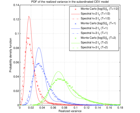
(a) The distribution of the realized variance in the subordinated CEV model.

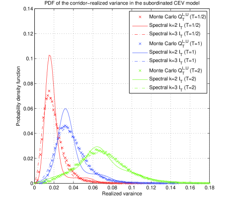
(b) The distribution of the corridor-realized variance in the subordinated CEV model.

Figure 3. Figure 3a (resp. 3b) contains the empirical probability distribution of the realized variance $[\log(S)]_{T}$ (resp. corridor-realized variance $Q^{L,U}_{T}(S)$, where $L=70$ and $U=130$) in the subordinated CEV model $S$, based on the Monte Carlo simulation described in the caption of Table 4 (see also Subsection 6.3). The distribution of the random variable $I_{T}$ for the maturity $T\in\{0.5,1,2\}$ matching $k\in\{2,3\}$ instantaneous moments is also plotted in both cases. For details on $I_{T}$ see Sections 2 and 5. The computational time required to obtain the law of $I_{T}$ is independent of $T$ and the quality of the approximation improves drastically for $k=3$ (see also Tables 7 and 8).

Table 7. The prices of volatility derivatives in the subordinated CEV model $S$. The parameter values for the process $S$ and the chain $X$ are given in the caption of Table 4. The parameters for the process $I$, the random variable $\Sigma_{T}$ and the payoffs of the volatility derivatives are as in Table 6. The algorithm described in the caption of Table 4 is used to generate $10^{5}$ paths of the process $S$ and the sum in (1) is used to obtain the empirical distribution of $[\log(S)]_{T}$ (see Figure 3a) and to evaluate the contingent claims in this table. The numbers in brackets are the standard errors in the Monte Carlo simulation. Note that the computational time for the pricing of volatility derivatives using the process $I$ is independent of the maturity $T$. All computations are performed on the same hardware as in Table 2 (the code in [14] can easily be adapted to this model).

Observe that the time required to compute the distribution of $I_{T}$ in the case of the continuous process $S$ (see Table 5) is larger than the time required to perform the equivalent task for the process with jumps (see Tables 6 and 7). From the point of view of the algorithm this difference arises because in the continuous case we have to use more points in the state-space of the process $I$ since condition (33) forces the choice of the smaller spacing $\alpha$. In other words the quotient $x\mapsto M_{2}(x)/M_{1}(x)$ takes much smaller values if there are no jumps in the model $S$ than if there are. It is intuitively clear from definition (8) that this ratio for the variance gamma (or the subordinated CEV) has a larger lower bound than the function in Figure 1b, because in the the diffusion case the generator matrix is tridiagonal.

CEV + jumps	$k$ moments		Spectral: $I_{T}$			MC: $Q^{L,U}_{T}(S)$
$\mathrm{derivative}\backslash T$		$0.5$	$1$	$2$	$0.5$	$1$	$2$
corr-var swap	1	19.81%	19.40%	18.50%	19.81%	19.41%	18.50%
$\sqrt{\mathbb{E}[\Sigma_{T}/T]}$	2	19.81%	19.40%	18.49%	(0.051%)	(0.050%)	(0.048%)
	3	19.81%	19.40%	18.50%
corr-vol swap	1	19.59%	19.22%	18.25%	19.12%	19.03%	18.19%
$\mathbb{E}\left[\sqrt{\Sigma_{T}/T}\right]$	2	19.18%	18.97%	18.08%	(0.016%)	(0.012%)	(0.005%)
	3	19.06%	18.93%	18.08%
Time			4s		100s	200s	400s

Table 8. Contingent claims on corridor-realized variance in the subordinated CEV model $S$. The corridor is defined by $L=70$ and $U=130$. All parameter values are as in Table 7. The empirical distribution of $Q^{L,U}_{T}(S)$ and the law of $I_{T}$ for $T\in\{0.5,1,2\}$ are given in Figure 3b. The Monte Carlo algorithm is as described in Table 4 and the numbers in brackets are the standard errors in the simulation.

Finally we apply our algorithm to computing the law of the corridor-realized variance $Q_{T}^{L,U}(S)$, where $S$ is the subordinated CEV process and the corridor is given by $L=70$ and $U=130$. It is clear from Figure 3b and the price of the square root payoff in Table 8 that the process $I$ defined by matching $k=3$ instantaneous moments of $Q^{L,U}_{T}(S)$ approximates best the entire distribution of the corridor-realized variance. However, if one is interested only in the value of the corridor variance swap (i.e. a derivative with a payoff that is linear in $Q^{L,U}_{T}(S)$), Table 8 shows that it suffices to take $k=1$.

7. Conclusion

We proposed an algorithm for pricing and hedging volatility derivatives and derivatives on the corridor-realized variance in markets driven by Markov processes of dimension one. The scheme is based on an order $k$ approximation of the corridor-realized variance process by a continuous-time Markov chain. We proved the weak convergence of our scheme as $k$ tends to infinity and demonstrated with numerical examples that in practice it is sufficient to use $k=2$ if the underlying Markov process is continuous and $k=3$ if the market model has jumps.

There are two natural open questions related to this algorithm. First, it would be interesting to understand the precise rate of convergence in Theorem 3.1 both from the theoretical point of view and that of applications. The second question is numerical in nature. As mentioned in the introduction, the algorithm described in this paper can be adapted to the case when the process $S$ is a component of a two dimensional Markov process. The implementation of the algorithm in this case is hampered by the dimension of the generator of the approximating Markov chain, which would in this case be approximately $2000$ (as opposed to $70$, as in the examples of Section 6). It would be interesting to understand the precise structure of this large generator matrix and perhaps exploit it to obtain an efficient algorithm for pricing volatility derivatives in the presence of stochastic volatility.

Appendix A Partial-circulant matrices

A matrix $C\in\mathbb{R}^{n\times n}$ is circulant if there exists a vector $c\in\mathbb{R}^{n}$ such that $C_{ij}=c_{(i-j)\!\!\!\mod n}$ for all $i,j\in\{1,\ldots,n\}.$ The matrix $C$ can always be diagonalised analytically, when viewed as a linear operator on the complex vector space $\mathbb{C}^{n}$, as follows. For any $r\in\{0,\ldots,n-1\}$ we have an eigenvalue $\lambda_{r}$ and a corresponding eigenvector $y^{(r)}$ (i.e. the equation $Cy^{(r)}=\lambda_{r}y^{(r)}$ holds for all $r$ and the family of vectors $y^{(r)}$, $r\in\{0,\ldots,n-1\}$, spans the whole of $\mathbb{C}^{n}$) of the form

$$\lambda_{r}=\sum_{k=0}^{n-1}c_{k}e^{-i\frac{2\pi}{n}rk}\quad\text{and}\quad y^{(r)}_{j}=\frac{1}{\sqrt{n}}e^{-i\frac{2\pi}{n}rj}\>\>\>\>\mathrm{for}\>\>\>\>j\in\{0,\ldots,n-1\}.$$

It is interesting to note that the eigenvectors $y^{(r)}$, $r\in\{0,\ldots,n-1\}$, are independent of the circulant matrix $C$. For the proof of these statements see Appendix A in [1].

Let $A$ be a linear operator represented by a matrix in $\mathbb{R}^{m\times m}$ and let $B^{(k)}$, for $k=0,\ldots,m-1$, be a family of $n$-dimensional matrices with the following property: there exists an invertible matrix $U\in\mathbb{C}^{n\times n}$ such that

$$U^{-1}B^{(k)}U=\Lambda^{(k)},\>\>\>\>\mathrm{for}\>\>\mathrm{all}\>\>\>\>k\in\{0,\ldots,m-1\},$$

where $\Lambda^{(k)}$ is a diagonal matrix in $\mathbb{C}^{n\times n}$. In other words this condition stipulates that the family of matrices $B^{(k)}$ can be simultaneously diagonalized by the transformation $U$. Therefore the columns of matrix $U$ are eigenvectors of $B^{(k)}$ for all $k$ between 0 and $m-1$.

Let us now define a large linear operator $\widetilde{A}$, acting on a vector space of dimension $mn$, in the following way. Clearly the matrix $\widetilde{A}$ can be decomposed naturally into $m^{2}$ blocks of size $n\times n$. Let $\widetilde{A}_{i,j}$ denote an $n\times n$ matrix which represents the block in the $i$-th row and $j$-th column of this decomposition. We now define the operator $\widetilde{A}$ as

(45) $$\widetilde{A}_{ii} := B^{(i)}+A_{ii}\mathbb{I}_{\mathbb{R}^{n}}\>\>\>\>\mathrm{and}$$

(46) $$\widetilde{A}_{ij} := A_{ij}\mathbb{I}_{\mathbb{R}^{n}},\>\>\>\>\mathrm{for}\>\>\mathrm{all}\>\>\>\>i,j\in\{1,\ldots,m\}\>\>\>\>\mathrm{such}\>\>\mathrm{that}\>\>\>\>i\neq j.$$

The real numbers $A_{ij}$ are the entries of matrix $A$ and $\mathbb{I}_{\mathbb{R}^{n}}$ is the identity operator on $\mathbb{R}^{n}$. We may now state our main definition.

Definition. A matrix is termed partial-circulant if it admits a structural decomposition as in (45) and (46) for any matrix $A\in\mathbb{R}^{m\times m}$ and a family of $n$-dimensional circulant matrices $B^{(k)}$, for $k=0,\ldots,m-1$.

For the spectral properties of partial-circulant matrices see Appendix A in [1].

Appendix B Non-uniform state-space of the Markov chain $X$

The task here is to construct a non-uniform state-space for the Markov chain $X$, which was used in Section 6 to approximate the Markov process $S$. Recall that the state-space is a set of non-negative real numbers $E=\{x_{0},x_{1},\ldots,x_{N-1}\}$ for some even integer $N\in 2\mathbb{N}$. Recall that the elements of the set $E$, when viewed as a finite sequence, are strictly increasing. We first fix three real numbers $l,s,u\in\mathbb{R}$, such that $l<s<u$, that specify the boundaries of the lattice $x_{0}=l$, $x_{N-1}=u$ and the starting point of the chain $x_{\lceil N/2\rceil}=s=S_{0}$ which coincides with the initial spot value in the model $S$. The function $\lceil\cdot\rceil:\mathbb{R}\to\mathbb{Z}$ returns the smallest integer which is larger or equal than the argument. We next choose strictly positive parameter values $g_{l},g_{u}$ which control the granularity of the spacings between $l$ and $s$ and between $s$ and $u$ respectively. In other words the larger $g_{l}$ (resp. $g_{u}$) is, the more uniformly spaced the lattice is in the interval $[l,s]$ (resp. $[s,u]$). The algorithm that constructs the lattice points is a slight modification of the algorithm in [19], page 167, and can be described as follows.

1. Compute $c_{1}=\mathrm{arcsinh}\left(\frac{l-s}{g_{l}}\right)$, $c_{2}=\mathrm{arcsinh}\left(\frac{u-s}{g_{u}}\right)$, $N_{l}=\lceil N/2\rceil$ and $N_{u}=N-(N_{l}+1)$.

2. Define the lower part of the grid by the formula $x_{k}:=s+g_{l}\mathrm{sinh}(c_{1}(1-k/N_{l}))$ for $k\in\{0,\ldots,N_{l}\}$. Note that $x_{0}=l,x_{N_{l}}=s$.

3. Define the upper part of the grid using the formula $x_{N_{l}+k}:=s+g_{u}\mathrm{sinh}(c_{2}k/N_{u})$ for $k\in\{0,\ldots,N_{u}\}$. Note that $x_{N-1}=u$.

References

- [1] C. Albanese, H. Lo, and A. Mijatović. Spectral methods for volatility derivative. to apper in Quantitative Finance.
- [2] C.Albanese and A. Mijatović. A stochastic volatility model for risk-reversals in foreign exchange. to appear in International Journal of Theoretical and Applied Finance.
- [3] P. Carr and R. Lee. Hedging variance options on continuous semimartingales. to appear in Finance and Stochastics.
- [4] P. Carr and K. Lewis. Corridor variance swaps. Risk, 17(2), February 2004.
- [5] P. Carr and D. Madan. Option valuation using the fast fourier transform. Journal of Computational Finance, pages 61–73, 1998.
- [6] P. Carr and D. Madan. Towards a theory of volatility trading. In R. Jarrow, editor, Volatility: New Estimation Techniques for Pricing Derivatives, Risk publication, pages 417–427. Risk, 1998.
- [7] P. Carr, D. Madan, H. Geman, and M. Yor. Pricing options on realized variance. Finance and Stochastics, 9(4):453–475, 2005.
- [8] N. Dunford and J.T. Schwartz. Linear operators Part II: Spectral theory. John Wiley & Sons, 1963.
- [9] S.N. Ethier and T.G. Kurtz. Markov processes: Characterization and convergence. John Wiley & Sons, 1986.
- [10] J. Gatheral. The volatility surface: a practitoner’s guide. John Wiley & Sons, Inc., 2006.
- [11] P. Glasserman. Monte Carlo Methods in Financial Engineering. Springer, 2004.
- [12] J. Hull. Options, futures and other derivatives. Pearson Education, 6th edition, 2006.
- [13] J. Jacod and A.N. Shiryaev. Limit theorems for stochastic processes, volume 288 of A Series of Comprehensive Studies in Mathematics. Springer-Verlag, 2nd edition, 2003.
- [14] H. Lo and A. Mijatović. An implementation in Matlab of the algorithm given in the paper “Volatility derivatives in market models with jumps”, 2009. see URL http://www.ma.ic.ac.uk/~amijatov/Abstracts/VolDer.html.
- [15] D. Madan, P. Carr, and E.C. Chang. The variance gamma process and option pricing. European Finance Review, 2(1):79–105, 1998.
- [16] A. Mijatović. Spectral properties of trinomial trees. Proc. R. Soc. A, 463:1681–1696, 2007.
- [17] R. S. Phillips. On the generation of semigroups of linear operators. Pacific Journal of Mathematics, 2(3):343–369, 1952.
- [18] P. Protter. Stochastic integration and differential equations. Springer, 2nd edition, 2005.
- [19] D. Tavella and C. Randall. Pricing Financial Instruments: the finite difference method. Wiley, 2000.