Dynamic susceptibilities of the single impurity Anderson model within an enhanced non-crossing approximation
Abstract
The single impurity Anderson model (SIAM) is studied within an enhanced non-crossing approximation (ENCA). This method is extended to the calculation of susceptibilities and thoroughly tested, also in order to prepare applications as a building block for the calculation of susceptibilities and phase transitions in correlated lattice systems. A wide range of model parameters, such as impurity occupancy, temperature, local Coulomb repulsion and hybridization strength, are studied. Results for the spin and charge susceptibilities are presented. By comparing the static quantities to exact Bethe ansatz results, it is shown that the description of the magnetic excitations of the impurity within the ENCA is excellent, even in situations with large valence fluctuations or vanishing Coulomb repulsion. The description of the charge susceptibility is quite accurate in situations where the singly occupied ionic configuration is the unperturbed ground state; however, it seems to overestimate charge fluctuations in the asymmetric model at too low temperatures. The dynamic spin excitation spectrum is dominated by the Kondo-screening of the impurity spin through the conduction band, i.e. the formation of the local Kondo-singlet. A finite local Coulomb interaction leads to a drastic reduction of the charge response as processes involving the doubly occupied impurity state are suppressed. In the asymmetric model, the charge susceptibility is enhanced for excitation energies smaller than the Kondo scale due to the influence of valence fluctuations.
pacs:
75.40.Gb,71.27.+a, 72.10.FkI Introduction
The single impurity Anderson model (SIAM) describes an impurity of localized -states with local Coulomb interaction embedded into a metallic host of non-interacting -band electrons.Anderson (1961) In its simplest version it discards the possibility of a complex orbital structure of the impurity and models the local -states through a two-fold degenerate -orbital. The Hamiltonian for the impurity reads
| (1) |
with () and the usual creation (annihilation) and number operators for -electron with spin , respectively. The local one-particle energy is given by , and the local Coulomb interaction is the usual density-density interaction proportional to the matrix element . The non-interacting conduction electrons are modeled by a single band of Bloch states with crystal momentum characterized by the dispersion relation ,
| (2) |
These two parts mix via a hybridization amplitude ,
| (3) |
The total Hamiltonian is then the sum of these three terms
| (4) |
Even though the thermodynamics of the model can be solved exactly within the Bethe ansatz method,Andrei et al. (1983); Wiegmann and Tsvelick (1983); Tsvelick and Wiegmann (1983a, b) dynamic quantities can in general not be obtained exactly and one has to rely on approximations. The SIAM has been extensively studied with various methods, including the numerical renormalization group (NRG),Wilson (1975); Krishna-murthy et al. (1980a, b); Bulla et al. (2008) the (dynamic) density-matrix renormalization group ((D-)DMRG),White (1992, 1993); Kühner and White (1999); Hallberg (2006) quantum Monte Carlo (QMC) methods Hirsch and Fye (1986); Rubtsov et al. (2005); Werner et al. (2006) and direct perturbation theory with respect to the hybridization.Keiter and Kimball (1971a, b); Grewe and Keiter (1981); Keiter and Morandi (1984) Especially with the development of the dynamical mean-field theory (DMFT),Georges et al. (1996) where the solution of an effective SIAM represents the essential step towards the solution of the correlated lattice system, the interest in accurate and manageable impurity solvers has increased.
In this work, we extend the well established enhanced non-crossing approximation (ENCA)Pruschke and Grewe (1989); Grewe et al. (2008); Holm and Schönhammer (1989); Keiter and Qin (1990a) to the calculation of the static and dynamic susceptibilities of the impurity. Like many other approximations formulated within the direct perturbation theory with respect to the hybridization,Grewe (1983); Kojima et al. (1984); Sakai et al. (1988); Anders (1995); Kroha et al. (1997); Haule et al. (2001); Grewe et al. (2008) the ENCA is thermodynamically conserving in the sense of Kadanoff and Baym.Baym and Kadanoff (1961); Baym (1962) It extends the usual non-crossing approximation (NCA) to finite values of the Coulomb repulsion via the incorporation of the lowest order vertex corrections, which are necessary to produce the correct Schrieffer-Wolff exchange coupling and the order of magnitude of the low energy Kondo scale of the problem. From the NCA it is well known that some pathological structure appears at the Fermi level below a pathology scaleKuramoto and Müller-Hartmann (1985); Bickers (1987) . The ENCA removes the cusps in spectral functions associated with this pathologyPruschke and Grewe (1989) and only a slight overestimation of the height of the many-body resonance at very low temperatures remains. As it will be shown in this work, the skeleton diagrams selected within the ENCA suffer from an imbalance between charge and spin excitations and overestimate the influence of charge fluctuations. Other than that, it has no further limitations.
Despite the known limitations of the NCA it has been widely applied to more complex situations due to the forthright possibility of extensions. For the SIAM out of equilibrium it is one of the few methods to incorporate nonequilibrium dynamics as well as many-body effects.Wingreen and Meir (1994) Complex orbital multiplets can be included in a straight-forward manner and connections to experimental data can be made.Ehm et al. (2007) However, incorporating finite values of may change the many-body features near the Fermi level considerably.Grewe et al. (2008, 2009) Therfore, a well tested extension of the ENCA in order to calculate susceptibilities at finite with the same accuracy as the spectra is desired. In particular, the calculation of lattice susceptibilities within DMFT Schmitt and Grewe (2005); Jarrell (1995); Schmitt (2008) needs a reliable strategy for an effective impurity, and the treatment of one- and two-particle excitations of the same footing is of paramount importance. Calculations of lattice susceptibilities and phase transitions of the Hubbard model with the ENCA as the impurity solver are presented elsewhere.Schmitt ; Schmitt (2008)
Compared to the “numerically exact” schemes like the renormalization group methods (RG), exact diagonalization (ED) or QMC, the direct perturbation theory has its advantages: (i) The approximations are free of systematic errors stemming from the discretization of the conduction band (RG and ED) or imaginary time (QMC). The continuum of band states is kept throughout the calculation, and dynamic Green functions are formulated with continuous energy variables. Thus, there are no discretization-artefacts Zitko and Pruschke (2009) and there is no need for artificial broadening parametersSakai et al. (1989); Bulla et al. (2001) or -averaging.Oliveira and Oliveira (1994); Campo and Oliveira (2005) (ii) The coupled integral equations for dynamic quantities, which have to be solved numerically, are formulated on the real frequency axis, which renders the non-trivial numerical analytic continuation of a finite set of Fourier coefficientsJarrell and Gubernatis (1996) or deconvolutionRaas and Uhrig (2005) unnecessary. The continuous-time quantum Monte Carlo approach (CTQMC)Werner et al. (2006) avoids a systematic Trotter-error (i) but it is still plagued with the occurrence of a negative sign-problem.Troyer and Wiese (2005)
The discretization errors (i) are of special importance for self-consistent calculations like the DMFT. There, the solution of an impurity model is used to construct a guess for the Green function of the lattice which is then used to yield a new effective “conduction band” for the impurity model. Errors in the treatment of the continuum of band states will be propagated by the iterative solution and may lead to an incorrect distribution of spectral weight.
The ENCA can be solved quite effectively on simple desktop computers, and is numerically not very demanding. Spectral functions can be calculated within some seconds to minutes while dynamic susceptibilities may take up to some hours. Additionally, it contains no free parameters and no fine-tuning is necessary. This makes it especially interesting for involved lattice calculations.
II Theory
II.1 Direct perturbation theory
In direct perturbation theory with respect to the hybridization term the “unperturbed” system is represented by the uncoupled () interacting impurity. This is diagonalized by the ionic many-body states
| (5) |
where the operators are projectors on the eigenstates and are diagonal versions of the so-called ionic transfer (or Hubbard) operators . For a simple -shell the quantum numbers characterize the empty , singly occupied with spin and doubly occupied impurity states with the corresponding unperturbed eigenvalues , and , respectively. Furthermore, the partition function and dynamic Green function are expressed in terms of a contour-integration in the complex plane,
| (6) | ||||
| (7) | ||||
with either a fermionic or bosonic Matsubara frequency depending on the type of the operators and . The contour encircles all singularities of the integrand, which are situated on the and axes in a mathematicalley positive sense. Performing the trace over the -electrons first, the reduced -partition function , the -electron one-body Green function and generalized susceptibility can be expressed as
| (8) |
| (9) | ||||
| (10) |
Here and the ionic propagators
| (11) | ||||
| (12) |
which describe the dynamics of an ionic state , are introduced. In equation (12) the ionic propagator is expressed with the help of the ionic self-energy . indicates that the trace is to be taken over the -states only, and represents the partition function of the isolated -system. In equations (9) and (10), and represent vertex functions to be specified later. These equations are graphically represented in Figure 1.

After re-writing the Hamiltonian in terms of the ionic transfer operators , the resolvent operator is expanded with respect to , . Consequently inserting the identity and using the representation (11) for the ionic propagators, this perturbation theory can be formulated with time-ordered Goldstone diagrams, representing the dynamics of the ionic states and their hybridization processes111 The ionic transfer operators can be avoided by enlarging the Hilbert space and introducing auxiliary slave-bosons, which represent the empty state, see Ref Coleman, 1984. The resulting standard Feynman perturbation-theory is in a one-to-one correspondence to the non-standard time-ordered Goldstone expansion described here..
Approximations are then introduced for the self-energies and vertex functions and . In order to be able to describe non-perturbative many-body phenomena like the Kondo effect, certain classes of diagrams have to be re-summed up to infinite order, resulting in a formulation in terms of skeleton diagrams, and corresponding coupled integral equations for the relevant dynamic functions. Deriving these equations consistently through functional derivatives from one Luttinger-Ward functional renders these approximations thermodynamically consistent.
II.2 ENCA for generalized dynamic susceptibilities
Within the ENCA, the ionic self-energies and propagators have to be determined from the well known set of coupled integral equations,Pruschke and Grewe (1989); Keiter and Qin (1990a); Saso (1992); Grewe et al. (2008)
| (13) | ||||
where the vertex functions are given by
| (14) | ||||
and . The hybridization function is constructed from the -band electrons
| (15) |
and is the Fermi function with the inverse temperature (note ).
For the generalized susceptibilities , an additional set of integral equations has to be set up which is shown graphically in Figure 2. In principle, there are 16 such functions, but for each quantum number only the four functions , , and are coupled. Due to the conserving nature of the ENCA, these equations are closely related to the ENCA expressions for the ionic self-energies; only some additional bosonic lines entering and leaving the site have to be introduced.
Whereas the lowest order vertex corrections of equation (14) together with the ionic propagators (11) and self-energies (12), are sufficient to furnish a conserving approximation, the vertices for the susceptibilities (10) have to be iterated up to infinite order! The transcription of these graphs into formulas is straight forward but lengthy and will be omitted here.

For very large Coulomb interactions the spectral weight in the doubly-occupied propagator is completely moved to energies of the order of . This leads to a negligible influence in the region of accessible energies of the order of the bandwidth due to the large energy denominators, and all terms involving effectively drop out of the equations. Therefore, for infinitely large Coulomb repulsion , the ENCA reduces to the usual NCA and all equations presented above approach the ones already known from the literature.Kuramoto (1983); Grewe (1983) In this sense, the ENCA is still referred to as non-crossing even though crossing diagrams are included. For approximations involving “real” crossing diagrams see Refs. Anders, 1995; Grewe et al., 2008; Kroha et al., 1997; Kroha and Wölfle, 2005.
The functions fulfill the symmetry relations
| (16) |
and
| (17) |
which are revealed by inspection of the perturbation expansion. The susceptibilities also obey the sum rules
| (18) | ||||
| (19) | ||||
| (20) |
which arise from the completeness relation of the local ionic states, . These sum rules transform into equivalent statements for the functions ,
| (21) |
It can be analytically checked that the ENCA respects these sum rules. The form of equation (21) explicitly reveals the conserving nature of this approximation, since the sum of sets of two-particle correlation functions is determined by the corresponding one-particle correlation function, i.e. the ionic propagator. Insofar the equations (21) resemble generalized Ward-Identities.
In order to obtain the physical susceptibility as a function of a real frequency, the contour integration of equation (10) has to be performed, and then the external bosonic Matsubara frequency can be analytically continued to the real axis, ( infinitesimal). The result of this procedure reads
| (22) | ||||
where the symmetry relations (16) were used and the defect quantities
| (23) |
were defined. Due to the appearance of the exponential factor, a direct numerical evaluation of the defect quantities given the is not possible, and additional sets of integral equations have to be solved for the (cf. Ref. Kuramoto and Kojima, 1984 and Kuramoto, 1986).
In the following, only spin-symmetric situations are considered, and the propagators for opposite spins are identified, i.e. , , ….
II.2.1 Magnetic susceptibility
The relevant quantity for the magnetic susceptibility is the auto-correlation function of the -component of the spin operator . This translates into the linear combination
| (24) |
which needs to be determined. Setting up the equations for this linear combination using the general equations depicted in Figure 2 leads to the cancellation of all spin-symmetric terms.Schmitt (2008) The function decouples from the and , and only one integral equation results,
| (25) | ||||
The derivation of the corresponding defect equation for along the lines of the definition (23) is straight forward, but will be omitted here for brevity.
II.2.2 Charge susceptibility
For the charge susceptibility the relevant quantity is the auto-correlation function of the charge operator leading to the dynamic function
| (26) | ||||
In the second equality sum rules like (21) were used. The function is not relevant for dynamic susceptibilities, since it only contributes in the case of a vanishing external frequency .
The hole susceptibility, i.e. the auto-correlation function of the hole operator , is given by the same expression, only with a different contribution from the sum rules. Both of these contributions do not change the dynamic susceptibility since they produce only the necessary constant shift between the static () charge and hole susceptibility after the contour integration,
| (27) |
The dynamical quantities of interest are best obtained by setting up the integral equations for the linear combinations , and , which read
| (28) | |||
| (29) | ||||
| (30) | |||
All three linear combinations are now coupled which makes the numerical solution of the full system inevitable.
The corresponding defect equations are again determined in a straight-forward way, but are omitted here due to their length.
II.3 Numerical evaluation
The ionic propagators and defect propagators are strongly peaked at the ionic threshold, and they even develop a singularity at zero temperature.Grewe et al. (2008); Kuramoto and Kojima (1984); Müller-Hartmann (1984) The position of this ionic threshold is not know exactly a priori, so we use self-generating adaptive frequency meshes to represent all functions numerically.
After obtaining the ionic propagators from the set of integral equations Eq. (13), Eqs. (25) and (28) – (30) can be solved to yield the two-particle quantities and . With these at hand, the corresponding defect equations can be solved and physical susceptibilities along the lines of Eq. (22) can be extracted.
All integral equations are solved via Krylov subspace methods,Saad (2000) where — starting from a sophisticated guess for the unknown functions — the equations are iterated until convergence is reached. In order to accelerate convergence and stabilize the iteration procedure Pulay-mixingPulay (1980) between different iterations is implemented (see, for example, Ref. Johnson, 1988 or Eyert, 1996).
Unfortunately, the system for the defect quantities becomes singular for vanishing external frequency . This is seen at the sum rule (21), which translates into implying that the become of the order of for small , while all terms in the integral equations stay at the order one. This becomes of some importance when extracting static susceptibilities from calculations of the dynamic susceptibilities, where a very small but finite frequency is used. The resulting convergence problems are probably connected to the ones already mentioned in Ref. Brunner and Langreth, 1997. More details on the numerics can be found in Ref. Schmitt, 2008.
III Results
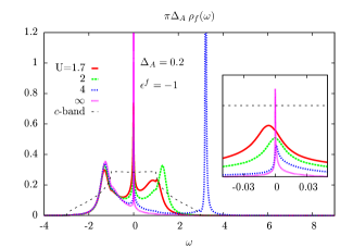
As it is well known, the SIAM exhibits the Kondo effect for sufficiently large Coulomb repulsion and the single particle level below the Fermi energy, . A very prominent manifestation of that effect is the emergence of the Abrikosov-Suhl resonance (ASR) in the one-particle density of states (DOS) at the Fermi level for temperatures of the order of the Kondo temperature . Within the ENCA an order of magnitude estimation for is given by Pruschke and Grewe (1989)
| (31) |
where is the effective antiferromagnetic Schrieffer-Wolff exchange coupling, the Anderson width and the half bandwidth of the conduction electron DOS . The hybridization matrix element was assumed to be local, i.e. momentum independent .
As already mentioned, the pathology of the NCA manifests itself in the overestimation of the height of the ASR and a violation of Fermi liquid properties for too low temperatures as well as in in situations with large valence fluctuations.Grewe (1983); Kuramoto and Kojima (1984); Kuramoto and Müller-Hartmann (1985); Bickers (1987) This pathological behavior is strongest for the case of a spin-only degeneracy (), which is considered in this work.
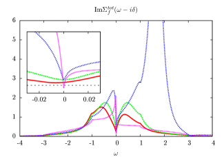
Figure 3 shows the one-particle -electron DOS and the imaginary part of the total self-energy Im calculated within the ENCA and the NCA (). As can be seen, the ENCA does not overestimate the height of the Kondo peak or violate the Fermi liquid property of the total self-energy Im down to temperatures of half the Kondo temperature. In contrast, the NCA curves in the graphs do violate these limits for the same parameter values.
The fact that the ENCA performs better than the NCA in comparable situations is a consequence of a better balance between different kinds of perturbational processes. The importance of such a balance has been pointed out repeatedly.Grewe et al. (2008); Keiter (1985); Keiter and Qin (1990b)
Even though the performance of the ENCA is considerably enhanced over the NCA, it eventually overestimates the height of the ASR for even lower temperatures and still misses to produce the correct Fermi liquid relations. Further improvements can be archived via the incorporation of higher-order diagrams.Grewe et al. (2008)
III.1 Benchmarking the ENCA
III.1.1 Static susceptibilities in the symmetric case
In order to obtain a better understanding of possible shortcomings of the ENCA it is worthwhile to consider charge and spin excitations separately and benchmark them against some exactly known results. The thermodynamics of the SIAM can be obtained exactly from the Bethe ansatz method.Kawakami and Okiji (1981); Wiegmann and Tsvelick (1983); Tsvelick and Wiegmann (1983a); Kawakami and Okiji (1983); Okiji and Kawakami (1982) At zero temperature and for the symmetric case () with a flat conduction band of infinite bandwidth () the static susceptibilities can even be obtained in closed form,Okiji and Kawakami (1982); Horvatic and Zlatic (1985a)
| (32) |
with
| (33) |
and
| (34) |
Apart from the small coupling correction in the exponent, exactly coincides with the Kondo temperature of equation (31).
In the graphs of Figure 4 the exact zero temperature magnetic (upper) and charge (lower) susceptibilities of equations (32) and (34) (solid red lines) are compared to the ENCA susceptibilities (blue dots) for as a function of . For the ENCA curves two characteristic temperatures and are chosen.
The characteristic exponential dependence of the magnetic susceptibility is essentially the same as for the exact Bethe ansatz result, but the absolute height is somewhat different. At the magnetic susceptibility is roughly of its zero temperature saturation value. However, at the susceptibility has almost saturated and the agreement with the -value is quite good.
The deviations for are due to the method used to extract the static susceptibilities: The static limit is obtained by evaluating the dynamic susceptibility at a small but finite external frequency, in our case . Since the ENCA represents a conserving approximation, the results obtained with this method agree with the static susceptibility obtained from a derivative of a thermodynamic potential, or solving separate equations as in Otsuki et al. (2006). This is valid as long as the minimal frequency is negligible compared to the lowest energy scale in the problem.
However, the Kondo temperature for is only of the order of and decreases for larger . The susceptibility calculated at then does no longer represent the static limit anymore, and the decrease seen in Figure 4 is produced, which is therefore not indicating a shortcoming of the ENCA method. The deviation can be cured by choosing a smaller value for the external frequency.
The charge susceptibility (lower graph in Figure 4) shows no significant temperature dependence for and and lies right on top of the exact result. The deviations for are explained in the same way as for the magnetic susceptibility described above.
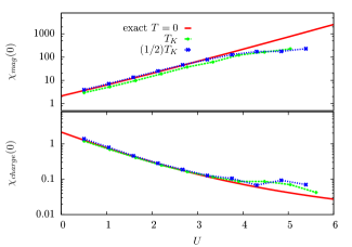
These reasons for the deviation at larger can be further confirmed by calculating the static susceptibilities for a fixed finite temperature as a function of the Coulomb interaction, which are shown in Figure 5. The figure compares the static magnetic (red dots) and charge (blue dots) susceptibilities for the symmetric situation with the exact results.
The charge susceptibility decreases monotonically with increasing Coulomb repulsion as expected. It follows the exact zero temperature susceptibility very accurately, which again confirms its weak temperature dependence in symmetric situations at low temperatures.
The magnetic susceptibility (red dots) does agree with the exact solution for low Coulomb repulsions but deviates for (). This is a finite temperature effect, since for values of the Kondo temperature is smaller than the chosen finite temperature of . Consequentlya, for we are not in the low temperature regime, and the susceptibility is not well described by its value. The magnetic susceptibility does not grow exponentially with as for , but instead saturates for at the asymptotic value of the Curie susceptibility of a free spin, , which is indicated by an arrow on the right border of the graph.
III.1.2 Static susceptibilities in the asymmetric case
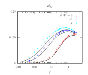
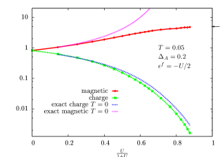
As a first test for the ENCA in the asymmetric situation Figure 6 compares the square of the effective screened local magnetic moment of the impurity,
| (35) |
to the exact Bethe ansatz result for three different ionic level positions as a function of temperature. The solid grey lines are the exact Bethe ansatz solution, which is taken from Ref. Okiji and Kawakami, 1983, while the colored points are ENCA calculations for the same parameter values. The half bandwidth was taken to be , which should be large enough to be comparable to the Bethe ansatz solution where .
The ENCA slightly overestimates the squared effective moment but all characteristic features are essentially the same as for the Bethe ansatz. Especially the shape and the relative height of the curves is in remarkable agreement: All three ENCA curves can be brought to lie right on top of the exact Bethe ansatz results when they are rescaled with one single factor. This indicates that the ENCA produces a slightly modified Kondo scale, but otherwise describes the static magnetic properties almost exactly. This is especially remarkable for the intermediate valence situation with , where the empty and singly occupied ionic configurations are almost degenerate. In such situations stronger pathologies occur in the one-particle DOS and the NCA-type of approximations would be expected to yield results of lower quality. However, as it can be seen, the magnetic excitations are still described very accurately.
Calculations of the effective squared local moments for a wide range of Coulomb interactions and hybridization strength (not shown) resemble the exact solutions known from the literature Krishna-murthy et al. (1980a, b); Okiji and Kawakami (1982) and the characteristics of the different asymptotic regimes are well reproduced by the ENCA.
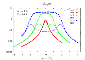
In Figure 7 the magnetic susceptibility is systematically examined as a function of the ionic level position and for fixed and . Also shown are the susceptibilities without explicit two-particle interactions (lines without dots labeled as “free”), i.e. the local particle-hole propagator calculated via
| (36) | ||||
where represents the one-particle -Green function (cf. equation (9)), the corresponding spectrum and the Fermi function.
All curves are symmetric around which just reflects the particle-hole symmetry of the model. The particle-hole propagators shows the expected maxima approximately situated at the positions of the Hubbard peaks in the one-particle DOS .
For very small , the susceptibility calculated with the ENCA is indistinguishable from the particle-hole propagator, as a consequence of the near lack of two-particle correlations.
For larger Coulomb interactions, the ENCA susceptibility shows only one broad maximum around (half filling), which grows in height and width with increasing . The enhancement of the susceptibility is due to the increasing local magnetic moment with larger . The plateau which develops around zero, is due to the stability of the local moment as long as the singly occupied ionic configuration is stable, i.e. the lower Hubbard peak being below and the upper above the Fermi level, and the temperature is not too low compared to . But as soon as one of the Hubbard peaks extends over the Fermi level, i.e. or , the moment is destabilized. For both Hubbard peaks below (above) the Fermi level, the impurity is predominantly doubly occupied (empty) and the magnetic susceptibility drops drastically. The curve then rapidly approaches the particle-hole propagator, indicating that explicit two-particle interactions are unimportant.
The reproduction of the correct results for the effectively non-interacting limit at as well as the empty- or fully occupied regimes is quite remarkable.
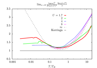
As it was already mentioned earlier, the NCA does violate Fermi liquid properties for very low temperatures. Another indication, in addition to the imbalance of the imaginary part of the total self energy at the Fermi level (-Im), stems from the zero frequency limit of the imaginary part of the dynamic susceptibility. For the Fermi liquid at it has to obey the so called Korringa-Shiba relationShiba (1975)
| (37) |
The function on the left hand side of this relation is shown in Figure 8 as a function of temperature for various values of . The explicit form (37) holds for a flat infinitely-wide conduction band DOS. For a different DOS the numerical pre-factors might change slightly, but the left-hand side is still expected to be of the order of unity due to universality of the SIAM at low energies.
For the NCA, the quantity Im is known to diverge at ,Müller-Hartmann (1984) which is reproduced by the curve in the figure. However, the ENCA (finite values) performs considerably better than the NCA. The curves still slightly increase for temperatures , but they eventually saturate at a finite value and do not diverge. This represents a considerable improvement of the qualitative behavior of the ENCA over the NCA.
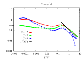
The temperature dependent static charge susceptibility is shown in the Figure 9 for various values of as a function of temperature. For high temperatures and the static susceptibility behaves effectively non-interacting with as expected.
For the susceptibility still has the characteristic dependence for high , but with a prefactor more closely to . This can be understood since in this situation the upper Hubbard peak (incorporating roughly half the spectral weight) is energetically just above the upper band edge of the -band and therfore the accessible spectral weight for two-particle excitations is approximately halved.
The rapid drop of the susceptibility for at temperatures is attributed to inaccuracies in the numerics for solving the integral equations. However, in this effectively non-interacting regime the susceptibility can be calculated without explicit two-particle interactions via the particle-hole propagator of equation (36). The results thus obtained are shown in the graph as colored dots without joining lines and are seen to be nicely proportional to for high temperatures.
Therefore, the ENCA nicely reproduces the high temperature asymptotics of the SIAM.
At temperatures around all susceptibilities show a pronounced maximum, which stems from thermally excited charge fluctuations between the empty and singly occupied ionic levels with excitation energy . For , fluctuations between the singly and doubly occupied states have the same excitation energy and therefore contribute equally. For the energy of fluctuations involving the doubly occupied state is somewhat smaller () and the peak is therefore broadened to lower energies. For the doubly occupied state is inaccessible for thermal fluctuations; so only the empty and singly occupied levels contribute leading to a reduction of the susceptibility maximum by approximately a factor of two.
At lower temperatures ( in the figures) the charge susceptibilities exhibit a slow increase followed by a saturation at the zero temperature values. The increase in the charge susceptibility occurs in a temperature range, where the Kondo singlet and the local Fermi liquid formation take place, which manifests itself in the growing many-body resonance at the Fermi level in one-particle DOS .
Even though a direct interpretation of the increase in terms of a Fermi liquid picture (where the charge susceptibility is proportional to the DOS at the Fermi level) is not applicable since the Fermi liquid is formed only at very low temperatures, it still provides an intuitive way of understanding: The increasing spectral weight at the Fermi level leads to an enlarged phase space volume for two-particle excitations and the charge susceptibility is at least roughly proportional to the DOS at the Fermi level. This is supported by the fact, that increases logarithmically with decreasing temperature, which is also the case for . But how strong the increase actually is and how it is influenced by the value of the Coulomb repulsion cannot be deduced from the simplified Fermi liquid analogy. This rather depends on the details of the two-particle correlations.
In the symmetric situation () the charge susceptibility increases only moderately and approaches the exact limiting value known from the Bethe ansatz, which is indicated by the arrow at the left border of the Figure 9. For the asymmetric cases, the increase is considerably more pronounced. Especially, the drastic low temperature increase for is rather unexpected. The absolute value of the susceptibility is even larger than for the smaller values of , which is counterintuitive since charge fluctuations should be suppressed for larger . However, the tendency that for a given level position the charge susceptibility in the asymmetric situation can increase with growing is known from perturbation theoryHorvatic and Zlatic (1985b) as a characteristic feature of valence fluctuation physics. Valence fluctuations being at the origin of this enhanced low temperature increase of the charge susceptibility are in agreement with the observation already made above, that for the doubly occupied ionic orbital is outside the conduction band and the system is therefore from the outset closer to the intermediate valence fixed point.
Reference calculations with the NRG (not shown) indeed display the characteristic features of the charge susceptibility as shown in Figure 9: A maximum for temperatures of the order of the ionic level positions and and an increase towards lower temperatures. In situations close to the valence fluctuation regime this increase leads to an enhancement of the charge susceptibility by a factor of about 10. However, the parameter values chosen for the ENCA-curve are not very close to the valence fluctuation fixed point. This is also reflected in the magnetic susceptibility for , which does not show any signatures of the valence fluctuation regime, but rather exhibits behavior characteristic for the transition from a local moment to the strong coupling fixed point (not shown). NRG calculations with parameter values similar to the ones chosen in this study, did show a low temperature increase, but not as strong as observed with the ENCA.
Altogether it can be concluded, that the ENCA does describe the charge fluctuations qualitatively right, but overestimates the influence of intermediate valence phenomena at very low temperatures in the asymmetric case.
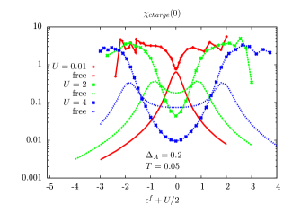
To make the range of applicability of the ENCA more clear, it is instructive to consider the charge susceptibility for fixed values of and , varying the ionic level positions , which is shown in Figure 10. The particle-hole propagators already displayed in Figure 7 are included as well (lines without dots). The ENCA charge susceptibilities are always minimal for half filling () and increases away from the symmetric case. The absolute value of the charge susceptibility in the symmetric situation is drastically reduced compared to the corresponding particle-hole propagator for large values and , which indicates, that the two-particle correlations strongly suppress charge fluctuations. In that situation, the susceptibility cannot accurately be described by the one-particle DOS alone and independent though strongly renormalized quasiparticles.
On the logarithmic scale, the increase with growing distance from zero can nicely be fitted with a parabola centered at zero, which corresponds to an exponential increase of the susceptibility, , . This shows the strong influence of the asymmetry and the contribution of valence fluctuations to the charge fluctuations.
However, the ENCA clearly fails for large asymmetries as the susceptibility saturates for 222Additionally, the numerics become unstable in these situations as it can be guessed from the strong fluctuations.. In contrast, should decrease again (cf. Kawakami and Okiji (1982)) and approach the particle-hole propagator, due to the effective non-interacting nature. This is most drastic for the almost non-interacting case with , where, apart from reproducing the value at half filling quite accurately, the curve goes the opposite direction as expected. The values at which the downturn in the susceptibility should occur correspond to situations, where both Hubbard peaks in the one-particle spectrum (very roughly at and ) are either below or above the Fermi level, corresponding to the empty- and fully occupied impurity regimes.
The ENCA is designed to describe spin flip scattering and the magnetic exchange coupling correctly but it does not fully capture the physics of charge fluctuations outside the Kondo regime. In situations, where the unperturbed ground state is either the empty or doubly occupied ionic state, crossing diagrams neglected in the ENCA are vital to describe charge fluctuations accurately. On the other hand, magnetic fluctuations are still described very accurately in these situations (see Figures 6 and 7).
III.2 Dynamic susceptibilities
III.2.1 Magnetic susceptibility
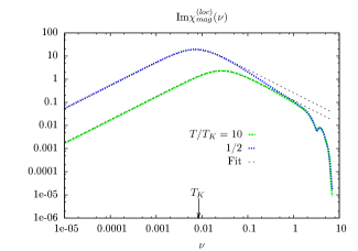
The imaginary part of the dynamic magnetic susceptibility is shown in Figure 11 for two different values of and two characteristic temperatures. The spectrum of the susceptibility shows a pronounced maximum, which is shifted to lower frequencies and increases considerably in height as the temperature is lowered. For temperatures below the Kondo temperature, the position of the maximum remains fixed at a value of the order of the Kondo temperature.
Also shown in the figure are fits with a Lorentzian form
| (38) |
which describe the low frequency susceptibilities very well. The form (38) corresponds to an exponential spin relaxation with relaxation time . The line-width is directly proportional to the NMR impurity nuclear spin-lattice relaxation rate .Shiba (1975)
The relaxation rates extracted from susceptibilities for various parameters follows a -lawSchmitt (2008) for high temperatures and saturates at a value of the order of at temperatures below (not shown), in accord with what was already found earlier.Bickers et al. (1987); Jarrell et al. (1991a); Anders (1995)
The physical picture behind these findings is quite clear: Upon lowering the temperature, the local moment of the impurity becomes increasingly coupled to the surrounding spin of the band electrons resulting in an enhanced response. At temperatures of the order of or lower than the Kondo temperature, the local Fermi liquid state is approached in which the local spin is screened and a local Kondo singlet is formed with a “binding energy” of about . Therefore the maximum in the spin excitations spectrum, as well as the NMR relaxation rate, both are pinned at an energy of the order of .
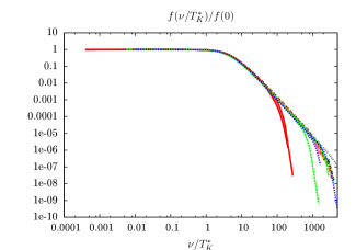
Jarrell et al. (1991a) also found that the function
| (39) |
shows universality and depends only on . Figure 12 shows this function normalized to its zero frequency value for various parameter sets. All graphs can be collapsed onto one single curve showing the universal shape of the function for low energies.
In order to achieve scaling a guess for the actual Kondo temperature has to be used. In contrast, the -value calculated by equation (31) and used in this work does not represent the exact physical low energy scale , but only provides an order of magnitude estimate. In the universal regime with a flat -band DOS this should not make any difference, but since we are using the 3d-SC DOS, non-universal corrections enter for different and . The value of the “real” Kondo temperature could have been extracted from fits of the calculated susceptibilities to the universal curve of the susceptibility as described by Jarrell et al. (1991b).
The rapid decrease of the curves in the figure for frequencies of also stems from the finite bandwidth of the 3d-SC conduction band used for these calculations.
The above findings clearly confirm, that the dynamics of the impurity spin is solely determined by the antiferromagnetic exchange between the impurity- and conduction electron spins. Even in the asymmetric situation, the only relevant energy scale for magnetic fluctuations of the impurity is the Kondo temperature at low temperatures.
III.2.2 Charge susceptibility
The imaginary part of the dynamic charge susceptibilities for two different Coulomb repulsions and characteristic temperatures, calculated with a 3d-SC band DOS, are shown in Figure 13. In the spectra the characteristic features stemming from excitations involving the Hubbard peaks at energies around and are clearly visible.
In the symmetric case (), the height of the peak at is about twice of the one in the asymmetric case (). This is due to the doubled phase-space volume for the symmetric situation with excitation energies matching, , while for the upper Hubbard peak is moved to higher energies.
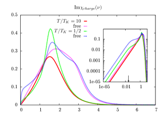
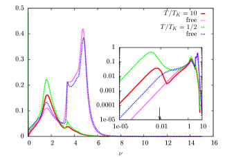
Also shown in the graphs are the local particle-hole propagators of equation (36) (labeled as “free”). These show characteristic features of the Hubbard peaks too, but the most prominent difference to the fully interacting susceptibility is the strong suppression of the high energy response in the latter. For example, the broad excitation continuum in the particle-hole propagator of the asymmetric case () for energies in the range is reduced to a very small peak at in the fully interacting susceptibility.
is just a measure for the phase space volume for statistical independent particle-hole excitations, which are described by the one-particle DOS . The quasiparticles and -holes at the Fermi level, on the other hand, are strongly correlated, leading to an effective suppression of the available phase space volume.
The role of the low energy quasiparticles can be studied by comparing the particle-hole propagator and the interacting susceptibilities at low energies for the symmetric situation (, inset). The response via the particle-hole propagator for shows an increase for lower temperatures, which stems from the quasiparticle-quasihole excitations within the growing Kondo resonance. In the fully interacting susceptibility this increase is approximately an order of magnitude smaller, clearly showing the effect of correlations in the two-particle response.
Surprisingly, for the asymmetric case () this trend is reversed and the interacting susceptibility is enhanced over the particle-hole propagator for excitation energies smaller than the Kondo scale (see inset). This very pronounced low energy response is produced by quasiparticle-quasihole excitations in the local Fermi liquid phase at low temperatures. The fact that these excitations are strongly enhanced in the asymmetric case compared to the symmetric situation is associated with the presence of strong valence fluctuations, as was already discussed for the static susceptibility above.
Even though such a low energy enhancement was not reported in NRG calculations for the charge susceptibilitySakai et al. (1989); Frota (1991) an inspection of the low energy part of the many-body spectrum obtained with the NRG Anders (2004) and preliminary NRG-calculations indeed suggest the possibility of an enhanced charge response for asymmetric situations.
A similar but not as strong temperature dependent increase in the dynamic susceptibility for temperatures of the order of the Kondo temperature was already found for larger orbital degeneracy and with the NCA .Brunner and Langreth (1997)
Therefore we argue, that these findings for the dynamic charge susceptibility are in accord with the ones discussed in the previous section for the static charge susceptibility. The observed increase of the charge response for energies smaller than the Kondo scale is indeed physical and due to the influence of the valence fluctuations of the low temperature Fermi liquid. However, the magnitude of the enhancement shown in Figure 13 is arguable, especially for the choice of parameters in the present calculation.
IV Conclusions
We have studied the SIAM within a conserving approximation, the ENCA, for a variety of model parameters. It was shown, that the ENCA constitutes a very accurate approximation for the static and dynamic one- and two-particle quantities of that model for temperatures down to a fraction of the Kondo temperature. It considerably improves the Fermi liquid properties and cures shortcomings of the (S)NCA, like the removal of the divergence of at zero temperature.
In symmetric situations (), the static magnetic and charge susceptibilities were shown to be in excellent agreement with the exact Bethe ansatz results. This was even true for cases with very small Coulomb interaction , which could not be expected from the beginning, since approximations within direct perturbation theory with respect to the hybridization usually have problems describing the non-interacting case.
The static magnetic susceptibility is in excellent agreement with exact Bethe ansatz results in the asymmetric situation. This holds also in cases with strong valence fluctuations, such as for or in the empty- and fully occupied orbital regimes.
However, the static charge susceptibility in the asymmetric model is described accurately only in situations, where the singly occupied impurity valence state represents the unperturbed () ground state. In addition, even though we believe that the qualitative features of the charge susceptibility in asymmetric situations are captured by the presented calculations, the influence of valence fluctuations is probably overestimated for too low temperatures. This confirms the expectation, that crossing diagrams, which are neglected in the ENCA, are essential for the quantitative description of situations with strong valence fluctuations, where the impurity occupation is statistically fluctuating. This also is in accord with the known pathologies in the one-particle spectral function. There, charge and magnetic fluctuations both contribute and the overestimation of the charge excitations at very low temperatures leads to the overshooting of the Kondo resonance and the observes spikes in the DOS.
The dynamic magnetic susceptibility is dominated by Kondo screening of the impurity spin. The ENCA correctly reproduces the temperature and other parameter dependencies of the magnetic excitations, and also the scaling found in previous studies is obtained.
The dynamical charge spectrum shows a severe suppression of high energy excitations due to correlations, when compared to the particle-hole propagator, which would represent the susceptibility of independent renormalized quasiparticles. Additionally the low energy response for excitation energies smaller than the Kondo temperature is also strongly suppressed in the symmetric case, due to the same correlations between low energy quasiparticles.
In the asymmetric situation the low energy charge response is drastically enhanced and an additional peak emerges. This enhancement is attributed to the presence of the valence fluctuation fixed point in the asymmetric model. Such an enhancement seems quite probable so that only the steepness of the increase calculated within the ENCA for parameter values chosen is arguable.
With these findings, the prospects of describing two-particle dynamics of lattice systems within the DMFT are very promising and results will be presented in a subsequent publication.Schmitt ; Schmitt (2008)
Acknowledgements.
The authors acknowledge fruitful discussions with E. Jakobi and F.B. Anders. One of us (SS) especially thanks F.B. Anders for providing him with his NRG code to perform the reference calculations mentioned in the text, and acknowledges support from the DFG under Grant No. AN 275/6-1.References
- Anderson (1961) P. W. Anderson, Phys. Rev. 124, 41 (1961).
- Andrei et al. (1983) N. Andrei, K. Furuya, and J. H. Lowenstein, Rev. Mod. Phys. 55, 331 (1983).
- Wiegmann and Tsvelick (1983) P. B. Wiegmann and A. M. Tsvelick, J. Phys. C 16, 2281 (1983).
- Tsvelick and Wiegmann (1983a) A. M. Tsvelick and P. B. Wiegmann, J. Phys. C 16, 2321 (1983a).
- Tsvelick and Wiegmann (1983b) A. Tsvelick and P. Wiegmann, Adv. Phys. 32, 453 (1983b).
- Wilson (1975) K. G. Wilson, Rev. Mod. Phys. 47, 773 (1975).
- Krishna-murthy et al. (1980a) H. R. Krishna-murthy, J. W. Wilkins, and K. G. Wilson, Phys. Rev. B 21, 1003 (1980a).
- Krishna-murthy et al. (1980b) H. R. Krishna-murthy, J. W. Wilkins, and K. G. Wilson, Phys. Rev. B 21, 1044 (1980b).
- Bulla et al. (2008) R. Bulla, T. Costi, and T. Pruschke, Rev. Mod. Phys. 80, 395 (2008).
- White (1992) S. R. White, Phys. Rev. Lett. 69, 2863 (1992).
- White (1993) S. R. White, Phys. Rev. B 48, 10345 (1993).
- Kühner and White (1999) T. D. Kühner and S. R. White, Phys. Rev. B 60, 335 (1999).
- Hallberg (2006) K. Hallberg, Adv. Phys. 55, 477 (2006).
- Hirsch and Fye (1986) J. E. Hirsch and R. M. Fye, Phys. Rev. Lett. 56, 2521 (1986).
- Rubtsov et al. (2005) A. N. Rubtsov, V. V. Savkin, and A. I. Lichtenstein, Phys. Rev. B 72, 035122 (2005).
- Werner et al. (2006) P. Werner, A. Comanac, L. de’ Medici, M. Troyer, and A. J. Millis, Phys. Rev. Lett. 97, 076405 (2006).
- Keiter and Kimball (1971a) H. Keiter and J. C. Kimball, J. Appl. Phys. 42, 1460 (1971a).
- Keiter and Kimball (1971b) H. Keiter and J. C. Kimball, Int. J. Magn. 1, 233 (1971b).
- Grewe and Keiter (1981) N. Grewe and H. Keiter, Phys. Rev. B 24, 4420 (1981).
- Keiter and Morandi (1984) H. Keiter and G. Morandi, Phys. Rep. 109, 227 (1984).
- Georges et al. (1996) A. Georges, G. Kotliar, W. Krauth, and M. J. Rozenberg, Rev. Mod. Phys. 68, 13 (1996).
- Pruschke and Grewe (1989) T. Pruschke and N. Grewe, Z. Phys. B 74, 439 (1989).
- Grewe et al. (2008) N. Grewe, S. Schmitt, T. Jabben, and F. B. Anders, J. Phys.: Condens. Matter 20, 365217 (2008).
- Holm and Schönhammer (1989) J. Holm and K. Schönhammer, Solid State Commun. 69, 969 (1989).
- Keiter and Qin (1990a) H. Keiter and Q. Qin, Physica B 163, 594 (1990a).
- Grewe (1983) N. Grewe, Z. Phys. B 53, 271 (1983).
- Kojima et al. (1984) H. Kojima, Y. Kuramoto, and M. Tachiki, Z. Phys. B 54, 293 (1984).
- Sakai et al. (1988) O. Sakai, M. Motizuki, and T. Kasuya, in Core-Level Spectroscopy in Condensed Systems Theory, edited by J. Kanamori and A. Kotani (Springer, Heidelberg, 1988), p. 45.
- Anders (1995) F. B. Anders, J. Phys.: Condens. Matter 7, 2801 (1995).
- Kroha et al. (1997) J. Kroha, P. Wölfle, and T. A. Costi, Phys. Rev. Lett. 79, 261 (1997).
- Haule et al. (2001) K. Haule, S. Kirchner, J. Kroha, and P. Wölfle, Phys. Rev. B 64, 155111 (2001).
- Baym and Kadanoff (1961) G. Baym and L. P. Kadanoff, Phys. Rev. 124, 287 (1961).
- Baym (1962) G. Baym, Phys. Rev. 127, 1391 (1962).
- Kuramoto and Müller-Hartmann (1985) Y. Kuramoto and E. Müller-Hartmann, J. Magn. Magn. Mater. 52, 122 (1985).
- Bickers (1987) N. E. Bickers, Rev. Mod. Phys. 59, 845 (1987).
- Wingreen and Meir (1994) N. S. Wingreen and Y. Meir, Phys. Rev. B 49, 11040 (1994).
- Ehm et al. (2007) D. Ehm, S. Hufner, F. Reinert, J. Kroha, P. Wolfle, O. Stockert, C. Geibel, and H. v. Lohneysen, Phys. Rev. B 76, 045117 (2007).
- Grewe et al. (2009) N. Grewe, T. Jabben, and S. Schmitt, Eur. Phys. J. B 68, 23 (2009).
- Schmitt and Grewe (2005) S. Schmitt and N. Grewe, Physica B 359-361, 777 (2005).
- Jarrell (1995) M. Jarrell, Phys. Rev. B 51, 7429 (1995).
- Schmitt (2008) S. Schmitt, Ph.D. thesis, TU Darmstadt (2008), URL http://tuprints.ulb.tu-darmstadt.de/1264/.
- (42) S. Schmitt, in preparation.
- Zitko and Pruschke (2009) R. Zitko and T. Pruschke, Phys. Rev. B 79, 085106 (2009).
- Sakai et al. (1989) O. Sakai, Y. Shimizu, and T. Kasuya, J. Phys. Soc. Jpn. 58, 3666 (1989).
- Bulla et al. (2001) R. Bulla, T. A. Costi, and D. Vollhardt, Phys. Rev. B 64, 045103 (2001).
- Oliveira and Oliveira (1994) W. C. Oliveira and L. N. Oliveira, Phys. Rev. B 49, 11986 (1994).
- Campo and Oliveira (2005) V. L. Campo and L. N. Oliveira, Phys. Rev. B 72, 104432 (2005).
- Jarrell and Gubernatis (1996) M. Jarrell and J. E. Gubernatis, Phys. Rep. 269, 133 (1996).
- Raas and Uhrig (2005) C. Raas and G. S. Uhrig, Eur. Phys. J. B 45, 293 (2005).
- Troyer and Wiese (2005) M. Troyer and U.-J. Wiese, Phys. Rev. Lett. 94, 170201 (2005).
- Saso (1992) T. Saso, Prog. Theor. Phys. Suppl. 108, 89 (1992).
- Kuramoto (1983) Y. Kuramoto, Z. Phys. B 53, 37 (1983).
- Kroha and Wölfle (2005) J. Kroha and P. Wölfle, J. Phys. Soc. Jpn. 74, 16 (2005).
- Kuramoto and Kojima (1984) Y. Kuramoto and H. Kojima, Z. Phys. B 57, 95 (1984).
- Kuramoto (1986) Y. Kuramoto, Z. Phys. B 65, 29 (1986).
- Müller-Hartmann (1984) E. Müller-Hartmann, Z. Phys. B 57, 281 (1984).
- Saad (2000) Y. Saad, Iterative Methods for Sparse Linear Systems (Cambridge University Press, 2000), 2nd ed.
- Pulay (1980) P. Pulay, Chem. Phys. Lett. 73, 393 (1980).
- Johnson (1988) D. D. Johnson, Phys. Rev. B 38, 12807 (1988).
- Eyert (1996) V. Eyert, J. Comput. Phys. 124, 271 (1996).
- Brunner and Langreth (1997) T. Brunner and D. C. Langreth, Phys. Rev. B 55, 2578 (1997).
- Keiter (1985) H. Keiter, Z. Phys. B 60, 337 (1985).
- Keiter and Qin (1990b) H. Keiter and Q. Qin, Z. Phys. B 79, 397 (1990b).
- Kawakami and Okiji (1981) N. Kawakami and A. Okiji, Phys. Lett. A 9, 483 (1981).
- Kawakami and Okiji (1983) N. Kawakami and A. Okiji, Solid State Commun. 43, 467 (1983).
- Okiji and Kawakami (1982) A. Okiji and N. Kawakami, Solid State Commun. 43, 365 (1982).
- Horvatic and Zlatic (1985a) B. Horvatic and V. Zlatic, J. Phys. 46, 1459 (1985a).
- Otsuki et al. (2006) J. Otsuki, H. Kusunose, and Y. Kuramoto, J. Phys. Soc. Jpn. Suppl. 75, 256 (2006).
- Okiji and Kawakami (1983) A. Okiji and N. Kawakami, Phys. Rev. Lett. 50, 1157 (1983).
- Shiba (1975) H. Shiba, Prog. Theor. Phys. 54, 967 (1975).
- Horvatic and Zlatic (1985b) B. Horvatic and V. Zlatic, Solid State Commun. 54, 957 (1985b).
- Kawakami and Okiji (1982) N. Kawakami and A. Okiji, J. Phys. Soc. Jpn. 51, 2043 (1982).
- Bickers et al. (1987) N. E. Bickers, D. L. Cox, and J. W. Wilkins, Phys. Rev. B 36, 2036 (1987).
- Jarrell et al. (1991a) M. Jarrell, J. E. Gubernatis, and R. N. Silver, Phys. Rev. B 44, 5347 (1991a).
- Jarrell et al. (1991b) M. Jarrell, J. Gubernatis, R. N. Silver, and D. S. Sivia, Phys. Rev. B 43, 1206 (1991b).
- Frota (1991) H. O. Frota, Phys. Rev. B 44, 8433 (1991).
- Anders (2004) F. B. Anders, Lecture Notes, Universität Bremen (2004).
- Coleman (1984) P. Coleman, Phys. Rev. B 29, 3035 (1984).