Dynamic correlation in high-harmonic generation for helium atoms in intense visible lasers

Abstract

We investigate the effect of dynamic electron correlation on high-harmonic generation in helium atoms using intense visible light ($\lambda=390$nm). Two complementary approaches are used which account for correlation in an approximate manner: time-dependent density-functional theory and a single-active-electron model. For intensities $I\sim 10^{14}$ W/cm², the theories are in remarkably good agreement for the dynamic polarization and harmonic spectrum. This is attributed to a low-frequency collective mode together with a high-frequency single-electron response due to the nuclear singularity, both of which dominate electron correlation effects. A time-frequency analysis is used to study the timing and emission spectrum of attosecond bursts of light. For short pulses, we find a secondary maximum below the classical cut-off. The imprint of the carrier-envelope phase, for the time-integrated spectral density appears at frequencies above the high-frequency drop-off, consistent with previous studies in the infrared $\lambda\sim 800$nm.

I Introduction

The development of sources of coherent ultrashort high-frequency light is a topic of great interest at present, with the prospect of illuminating ultrafast electron dynamics fohlisch05 ; he07 ; ruiz06 . Over the past decade, high-order harmonic generation (HHG) has been used as an extreme ultra-violet light source for a wide range of applications, and is a practical method for producing attosecond bursts from intense infrared lasers hentschel01 ; paul01 ; balt03 . In this scheme, an intense laser is focused into a gas target and the high-order nonlinearity of the response of the atoms provides a narrow, forward-beam of high-order harmonics. The efficiency of this process depends upon the individual atom susceptibility and the phase matching within the gas sample. Experiments based on this technique have led to generation of harmonics from rare-gas atoms with an infrared pump laser in excess of the 300th harmonic, using very short laser pulses ($<$ 20 femtoseconds) and peak intensities in excess of $I\sim 10^{14}$ W/cm² chang ; speilmann .

Interest is focusing on how these attosecond bursts might be controlled and optimized for applications in ultrafast spectroscopy. Availability of intense femtosecond lasers has driven research into the highly nonlinear response of atoms and molecules to extreme dynamic fields. The experimental tool of choice has been the Ti:Sapphire laser operating in the near infrared. Recently attention has turned to the use of frequency-doubled sources. Naturally, at very high intensities, $I>10^{15}$ W/cm², double ionization is a feature of the interaction. However, at intermediate intensities, ionization is a much weaker channel and, to a good approximation, the process is governed by single-electron excitation, possibly leading to single ionization. However, even in this case, one would expect the electron pair to retain aspects of correlation intrinsic to the unperturbed helium atom. The effect of correlation is a fundamental aspect of atomic structure, but its role in terms of hyperpolarizability and high-harmonic generation is not fully understood.

Dynamic correlation in helium can be treated exactly through the direct approach of solving the two-electron time-dependent Schrödinger equation (TDSE)

$$i\frac{\partial}{\partial t}\Psi(\mbox{\boldmath$r$}_{1},\mbox{\boldmath$r$}_{2},t)=H\Psi(\mbox{\boldmath$r$}_{1},\mbox{\boldmath$r$}_{2},t),$$ (1)

where $H$ is the Hamiltonian operator of the system. The solution embodies the dynamic polarizability that is the source of the high-frequency harmonics of interest. This partial-differential equation is intractable (in computational terms) for more than two electrons and even in the simple two-electron case, it requires several hundred processors to obtain a numerical solution when infrared wavelengths are considered parker98 . The reason for these large computational demands is due to the treatment of the electron-electron correlation term. In the case of stationary or metastable states of the helium atom, this correlation term can be accounted for, in an essentially exact manner, using basis function expansions. However, under transient perturbations, the dynamic correlation of the atom is more problematic. Nonetheless, the problem is well known and consequently this equation has received a great deal of attention, not least because of its importance in ion-atom collisions in gases and plasmas parker07 ; parker06 ; lambropoulos05 ; nikolopoulos06 .

In this paper, we investigate the role of electron correlation, by using two semi-correlated approaches. More precisely, we use two different models which account for correlation in an approximate manner. The methods employed to solve this equation are a time-dependent density functional theory (TDDFT) approach, recently developed to study laser-molecule and laser-cluster interactions dundas:2004 and a single-active-electron (SAE) model tong05 . In this paper, we study the dependence of harmonic generation from helium on the intensity and carrier-envelope phase (CEP), both of which have been identified as being important physical parameters in the determination of HHG emission properties.

In Sec. II below, we introduce the TDDFT approach within the exchange-only limit, and provide numerical details for solving the corresponding time-dependent Kohn-Sham (TDKS) equations. In Sec. III, we describe the SAE method employed. In Sec. IV, we briefly mention how the power spectrum is calculated and illustrate how a time-frequency analysis is performed. Finally we discuss and summarize the results for HHG in helium. Atomic units are used throughout unless otherwise stated.

II TDDFT method

The TDDFT method has been applied extensively to the study of atomic and molecular systems driven by external laser pulses chu1 ; dreizler:1990 ; Uhlmann ; dundas:2004 ; Calvayrac ; castro:2004 ; otobe:2004 . Indeed TDDFT provides one of the most detailed, practical and feasible ab initio approaches for tackling many-body problems. The time-dependent formulation of ground-state density functional theory (DFT) hohenberg:1964 ; kohn:1965 was provided by Runge and Gross runge:1984 , who showed that the response of a system of interacting electrons could be obtained from that of a set of fictitious non-interacting particles exposed to a time-dependent local effective potential. As well as providing a method for studying the time-dependent evolution of an electronic system, it also allows for the calculation of excited state properties of static systems. Like TDDFT, many-body effects are in principle included exactly through an exchange-correlation functional; in practice the form of this functional is unknown and at best it can only be approximated.

Our implementation of TDDFT, as applied to a general spin-polarized system of $N$ electrons is set out in reference dundas:2004 . In the following we describe how our approach is applied to the two-electron atom. The Kohn-Sham wavefunction is written as a single determinant of one-particle Kohn-Sham orbitals. Since helium, initially in its ${}^{1}S^{e}$ ground state, is spin degenerate then only one Kohn-Sham orbital, $\psi_{\textrm{KS}}(\mbox{\boldmath$r$},t)$, is required. The electron spin densities are then equal, i.e.

$$n_{\uparrow}(\mbox{\boldmath$r$},t)=n_{\downarrow}(\mbox{\boldmath$r$},t)=\left|\psi_{\textrm{KS}}(\mbox{\boldmath$r$},t)\right|^{2},$$ (2)

where $\downarrow,\uparrow$ denotes the spin state of each electron, and so the total electron density is

$$n(\mbox{\boldmath$r$},t)=n_{\uparrow}(\mbox{\boldmath$r$},t)+n_{\downarrow}(\mbox{\boldmath$r$},t)=2\left|\psi_{\textrm{KS}}(\mbox{\boldmath$r$},t)\right|^{2}.$$ (3)

The time evolution of this orbital is governed by the TDKS equation

$$i\frac{\partial}{\partial t}\psi_{\textrm{KS}}(\mbox{\boldmath$r$},t)=H_{\textrm{KS}}\,\psi_{\textrm{KS}}(\mbox{\boldmath$r$},t),$$ (4)

where

$$H_{\textrm{KS}}(\mbox{\boldmath$r$},t)=-\frac{1}{2}\nabla^{2}+V_{\textrm{ext}}(\mbox{\boldmath$r$},t)+\int d\mbox{\boldmath$r$}^{\prime}\frac{n(\mbox{\boldmath$r$}^{\prime},t)}{|\mbox{\boldmath$r$}-\mbox{\boldmath$r$}^{\prime}|}+V_{xc}(\mbox{\boldmath$r$},t).$$ (5)

In equation (5) the external potential is given by

$$V_{\textrm{ext}}(\mbox{\boldmath$r$},t)=V_{\textrm{ion}}(\mbox{\boldmath$r$})+V_{\textrm{laser}}(\mbox{\boldmath$r$},t),$$ (6)

where $V_{\textrm{ion}}(\mbox{\boldmath$r$},t)$ and $V_{\textrm{laser}}(\mbox{\boldmath$r$},t)$ represent the Coulomb and laser-interaction terms respectively. We consider a linearly polarized laser pulse, make the dipole approximation and consider both the length and velocity form of the interaction. In a length-gauge description, the interaction term is given by

$$V^{(L)}_{\textrm{laser}}(\mbox{\boldmath$r$},t)=\mbox{\boldmath$r$}\cdot\hat{\mbox{\boldmath$e$}}\,E(t),$$ (7)

where $\hat{e}$ is the polarization direction. In the velocity gauge, the interaction term is

$$V^{(V)}_{\textrm{laser}}(\mbox{\boldmath$r$},t)=iA(t)\mbox{\boldmath$\hat{e}$}\,\cdot\mbox{\boldmath$\nabla$},$$ (8)

where $A(t)$ is the vector potential defined by

$$A(t)=A_{0}f(t)\cos(\omega_{L}t+\varphi),$$ (9)

and where $\omega_{L}$ is the frequency, $\varphi$ the carrier-envelope phase (CEP) and $f(t)$ the pulse envelope given by

$$f(t)=\left\{\begin{array}[]{lll}\sin^{2}(\pi t/T)&{0\leq t\leq T},\\[14.22636pt] 0&{\rm otherwise}\end{array}\right.$$

for a pulse of duration $T$. With this form of the vector potential, the electric field is

$$E(t)=E_{0}f(t)\sin(\omega_{L}t+\varphi)-\frac{E_{0}}{\omega_{L}}\frac{\partial f(t)}{\partial t}\cos(\omega_{L}t+\varphi).$$ (10)

The electric field amplitude ($E_{0}=\omega_{L}A_{0}$) is related to the cycle-average intensity $I$ by $E_{0}=\left(8\pi I/c\right)^{1/2}$, where $c$ is the speed of light. Similarly we define the ponderomotive energy, $U_{P}=E_{0}^{2}/(4\omega_{L}^{2})$.

The third term on the right-hand side of equation (5) represents the Hartree potential and the fourth term incorporates the remaining exchange and correlation effects. This exchange-correlation potential is itself spin-degenerate for helium and can be written as

$$V_{xc}(\mbox{\boldmath$r$},t)=V_{xc\sigma}(\mbox{\boldmath$r$},t)=\left.\frac{\delta E_{xc}[n_{\uparrow},n_{\downarrow}]}{\delta n_{\sigma}}\right|_{n_{\sigma}=n_{\sigma}(\mbox{\scriptsize\boldmath$r$},t)},$$ (11)

where $E_{xc}[n_{\uparrow},n_{\downarrow}]$ is the exchange-correlation action.

A crucial element in our model is the functional form of the exchange-correlation potential. While many sophisticated approximations to this potential have been developed functionals , the simplest is the adiabatic local density approximation in the exchange-only limit (xLDA). The exchange energy functional is then given by

$$E_{x}[n_{\uparrow},n_{\downarrow}]=-\frac{3}{2}\left(\frac{3}{4\pi}\right)^{1/3}\sum_{\sigma=\uparrow,\downarrow}n_{\sigma}^{4/3}(\mbox{\boldmath$r$},t),$$ (12)

from which the exchange-only potential

$$V_{x\sigma}(\mbox{\boldmath$r$},t)=-\left(\frac{6}{\pi}\right)^{1/3}n_{\sigma}^{1/3}(\mbox{\boldmath$r$},t),$$ (13)

is obtained. While this approximate functional is simple to implement it does suffer from the drawback of containing long-range self-interaction errors: the asymptotic form of the potential is exponential instead of Coulombic. The anomalous long-range form of the self-interaction potential means that the spectrum of single-particle highly-excited states are incorrect. It follows that physical multiphoton resonances, or alternatively (at extremely high intensities) the tunneling process, leading to ionization, will be poorly represented. Nevertheless, as we will see, the gross electrical properties of the atom are fairly well reproduced.

Since we consider a linearly-polarized laser pulse within the dipole approximation, rotational symmetry around the $z$-axis is preserved at all times, and so it is appropriate to solve the TDKS equation using cylindrical coordinates. The electron position vector is then given by

$$\mbox{\boldmath$r$}=\rho\cos\phi\mbox{\boldmath$i$}+\rho\sin\phi\mbox{\boldmath$j$}+z\mbox{\boldmath$k$}.$$ (14)

Precise numerical details of how the code is implemented are given in dundas:2004 . As in Dundas2 a finite difference treatment of the $z$-coordinate and a Lagrange mesh treatment of the $\rho$-coordinate based upon Laguerre polynomials is employed. The time-dependent Kohn-Sham equation is discretized in space using these grid techniques and the resulting computer code optimized to run on massively-parallel processors. Several parameters in the code affect the accuracy of the method and these are adjusted pragmatically until convergence is obtained. Specifically, these parameters are the number of points in the finite difference grid ($N_{z}$), the finite difference grid spacing ($\Delta z$), the number of Lagrange-Laguerre mesh points ($N_{\rho}$), the scaling parameter of the Lagrange-Laguerre mesh ($h_{\rho}$), the order of the time propagator ($N_{t}$) and the time spacing ($\Delta t$) dundas:2004 . In all the calculations presented here, converged results were obtained using the following parameters: $N_{z}=4485$, $\Delta z=0.02$, $N_{\rho}=60$, $h_{\rho}=0.2027685$, $N_{t}=18$ and $\Delta t=0.01$. Incidentally, these parameters, without any further adjustment, give converged (better than 1%) TDDFT orbital energies for the complete first-period of elements of the periodic table.

III SAE method

The single-active-electron (SAE) model watson97 ; watson972 ; kulander92 ; preston96 is, perhaps, the simplest and most appealing approach for multiphoton ionization in which a single valence electron is released. The model provides results that are cheaply produced, often to a very satisfactory degree of agreement with experiment and/or highly-expensive complex many-body calculations. As such, the model provides a useful benchmark in the absence of more sophisticated calculations or accurate measurements. We choose to employ spherical coordinates with the polar axis along the direction of linear polarization. The radius, $r$, and polar angle, $\theta$, are treated explicitly, whereas $\phi$ is treated analytically. Thus the field-free Hamiltonian, $H_{0}$, for the single-active-electron, of the helium atom initially in its ground-state can be written as

$$H_{0}(r,\theta) = -{1\over 2}\left[{1\over r^{2}}{\partial\over\partial r}\left(r^{2}{\partial\over\partial r}\right)\right.$$ (15)

$$+ \left.{1\over r^{2}\sin\theta}{\partial\over\partial\theta}\left(\sin\theta{\partial\over\partial\theta}\right)\right]+V(r),$$

where the model potential $V(r)$ we chose has the form of that calculated by Tong and Lin tong05

$$V(r)=-\frac{Z+a_{1}e^{-a_{2}r}+a_{3}re^{-a_{4}r}+a_{5}e^{-a_{6}r}}{r},$$ (16)

in which, $Z=1.0$, $a_{1}=1.231$, $a_{2}=0.662$, $a_{3}=-1.325$, $a_{4}=1.236$, $a_{5}=-0.231$ and $a_{6}=0.480$. In this expression, the long-range monopole $Z=1$ is supplemented by short-range corrections, $\{a_{i}\}$ expressing static correlation. The form of the potential was obtained from fitting to a self-interaction-free density functional. The Hamiltonian for the interacting system can be written in the form

$$H_{\textrm{SAE}}(r,\theta,t)=H_{0}(r,\theta)+V_{\textrm{laser}}(r,\theta,t).$$ (17)

The velocity gauge formulation is computationally attractive since the number of partial waves required for convergence is greatly reduced compared to the length-gauge. This also provides us with a check on the length-gauge results.

The TDSE defined by equation (1) therefore takes the form

$$H_{\textrm{SAE}}(r,\theta,t)\psi_{\textrm{SAE}}(r,\theta,t)=i\frac{\partial}{\partial t}\psi_{\textrm{SAE}}(r,\theta,t).$$ (18)

The SAE wavefunction, $\psi_{\textrm{SAE}}(r,\theta,t)$, is expanded in a direct product of radial and angular functions. The solid-angle normalized Legendre polynomials $Y_{l}^{0}(\theta)$ are efficient for the angular dimension, leading to a sparse interaction matrix. The radial coordinate is discretized using $B$-spline functions deb78 , so that

$$\psi_{\textrm{SAE}}(r,\theta,t)=\sum_{n=0}^{n_{\rm max}}\sum_{l=0}^{l_{\rm max}}c_{nl}(t)\frac{B^{k}_{n}(r)}{r}Y_{l}^{0}(\theta),$$ (19)

with $k$ the order of the splines, and where the expansion is truncated by a maximum angular momentum $l_{\rm max}$ and the limiting number of spline functions $n_{\rm max}$. This allows us to apply Dirac’s variation of constants method to the evolution. Taking inner products over the spatial basis functions we obtain a large set of ordinary, coupled first-order differential equations for the constants, $c_{nl}(t)$, in the form

$$\mbox{\boldmath$S$}\dot{\mbox{\boldmath$c$}}(t)=-i\mbox{\boldmath$H$}(t)\mbox{\boldmath$c$}(t),$$ (20)

where the overlap matrix $S$ is due to the non-orthogonality of the $B$-splines

$$S_{n^{\prime}l^{\prime},nl}=\delta_{l^{\prime}l}\times\int_{0}^{r_{\rm max}}drB^{k}_{n^{\prime}}(r)B^{k}_{n}(r),\quad|n^{\prime}-n|<k.$$ (21)

The interaction matrix is of the form

$$H_{n^{\prime}l^{\prime},nl}=2\pi\int_{o}^{\pi}d\theta\sin\theta\,\int_{0}^{r_{\textrm{max}}}dr\,rB_{n^{\prime}}^{k}(r)Y_{l^{\prime}}^{0}(\theta)\,H_{\textrm{SAE}}\,r^{-1}B_{n}^{k}(r)Y_{l}^{0}(\theta).$$ (22)

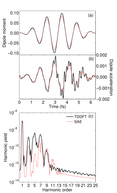
$I$ = 1 $\times$ 10¹⁴ W/cm²

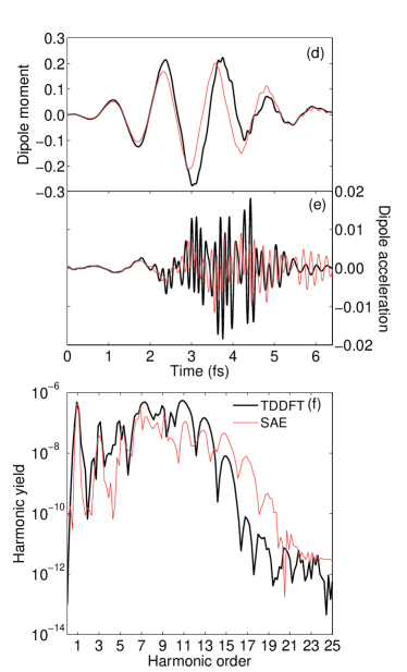
$I$ = 5 $\times$ 10¹⁴ W/cm²

Figure 1: (Color online) Generation of high-order harmonics in a helium atom exposed to a five cycle (6.4fs) linearly polarized laser pulse of wavelength $\lambda$ = 390nm for two different models: a TDDFT model (black lines) and a SAE model (red lines). The plots on the left-hand-side correspond to a laser intensity of $I$ = 1 $\times$ 10¹⁴ W/cm² while the plots on the right-hand-side correspond to a laser intensity of $I$ = 5 $\times$ 10¹⁴ W/cm². Sub-plots (a) and (d) present the dipole moment, (b) and (e) the dipole acceleration, and (c) and (f) the spectral density. There is remarkably close agreement between the TDDFT and SAE models. The dipole (center-of-charge) motion is consistently reproduced in phase and amplitude as can be seen from the dipole moment sub-plots. The irregular fluctuations in the dipole acceleration are also remarkably similar with a very efficient conversion of the 7th harmonic, extending to the 13th harmonic at the higher intensity. The oscillations in (e) for the SAE model after the pulse are due to $1s-2p$ fluorescence. There is negligible ionization for both models at the two intensities considered: less than 0.1% for $I$ = 1 $\times$ 10¹⁴ W/cm² and less than 2% for $I$ = 5 $\times$ 10¹⁴ W/cm². Instead of a classical plateau and cutoff, we have a dip and secondary maximum below the classical cut-off $\omega_{c}$: equation (28).

The theory and applications of $B$-splines are well known bac01 ; deb78 , but we briefly summarize their use for this problem. $B$-spline functions are localized overlapping piecewise polynomials designed to reproduce the radial oscillations of the wavepacket. These overlaps give rise to a narrow-banded symmetric structure in $S$, and by design, these elements can be evaluated exactly by Gauss-Legendre quadrature. A suitable choice of spline order, $k$, is governed by the Hamiltonian, and the radial space, $0\leq r\leq r_{\rm max}$, subdivided in sectors or scaled to vary the density of points, accordingly. Specifically, we discovered that $k=9$ order functions combine the advantages of low bandwidth and accurate representation of the wavefunction oscillations.

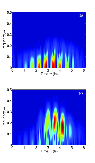
TDDFT

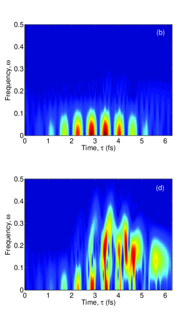
SAE

Figure 2: (Color online) Time-frequency analysis of high-order harmonic emission in a helium atom exposed to a five cycle (6.4fs) linearly polarized laser pulse of wavelength $\lambda$ = 390nm for two different models: a TDDFT model (left-hand plots) and a SAE model (right-hand plots). The spectral density of the STFT (equation(26)) is plotted as a function of the auxiliary time $\tau$; high density is colored red and low density blue. Two laser intensities were considered: sub-plots (a) and (b) correspond to $I=1\times 10^{14}$ W/cm² while sub-plots (c) and (d) correspond to $I=5\times 10^{14}$ W/cm².

The ground-state eigenvector is calculated and normalized to provide the stationary initial state $\mbox{\boldmath$c$}(0)$. Its evolution is then calculated by numerical solution of the system of equations (20). This is not a trivial task given the scale of the problem (the size of the interaction matrix) and the instabilities of the equations. It is well known that the choice of gauge has a strong effect on the dynamical terms in the matrices. Not surprisingly, this computational challenge has attracted a great deal of attention. While there exists a variety of tried and tested strategies for such problems, we have developed our own computer codes that treat the problem in complementary ways for both length and velocity gauges. This double approach provides both a numerical validation for the physical results, and allows us to select the more efficient method when required.

All calculations were performed with the PYPROP package pyprop , which is designed to provide a general interface for solution of the time-dependent Schrödinger equation. Discretization schemes and propagation methods are implemented following a standard interface, which enables users to test different methods without requiring detailed knowledge about the implementation. PYPROP is written in Python, while all the computationally-intensive routines have been developed in C++, using the blitz++ array library blitz . Depending on the problem at hand, the size of the grid and number of employed grid points will vary. For the range of angular momenta, we found that $l_{\rm max}=20$ was more than sufficient for convergence in all cases considered here. In addition we found that 1050 B-splines were sufficient for convergence. Time propagation was carried out using the Arnoldi method par86 .

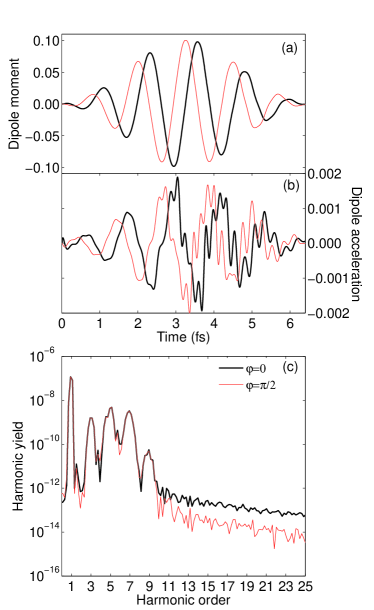
TDDFT: $I$ = 1 $\times$ 10¹⁴ W/cm²

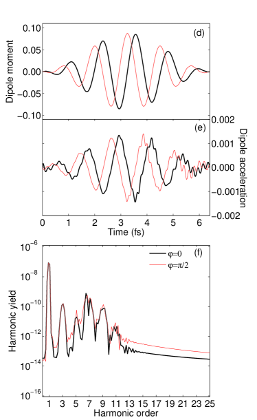
SAE: $I$ = 1 $\times$ 10¹⁴ W/cm²

Figure 3: (Color online) The effect of carrier-envelope phase (CEP), $\varphi$, on harmonic generation in a helium atom exposed to a five cycle (6.4fs) linearly polarized laser pulse of wavelength $\lambda$ = 390nm and intensity $I$ = 1 $\times$ 10¹⁴ W/cm² for two different models: a TDDFT model (left-hand plots) and a SAE model (right-hand plots). A pulse envelope defined by equation (10) was used and two CEP values were considered: $\varphi=0$ (black lines) and $\varphi=\pi/2$ (red lines). Sub-plots (a) and (d) present the dipole moment, (b) and (e) the dipole acceleration, and (c) and (f) the spectral density. We note that, for both models, there is very little effect of CEP in the time-integrated spectral density.

IV Frequency Analysis

The dipole moment is defined as

$$d(t) = -\int n(\mbox{\boldmath$r$},t)\,z\,d^{3}\mbox{\boldmath$r$},$$ (23)

$$= -2\langle\psi(t)|z|\psi(t)\rangle.$$

According to Larmor’s formula, the radiated power is proportional to the square of the dipole acceleration. This can be obtained using Ehrenfest’s theorem as burnett92

$$\ddot{d}(t)=-2\langle\psi(t)|[H,[H,z]]|\psi(t)\rangle.$$ (24)

The spectral density is then obtained as follows

$$S(\omega)=\left|\int_{0}^{T}\ddot{d}(t)e^{i\omega t}dt\right|^{2}.$$ (25)

TDDFT: $I$ = 5 $\times$ 10¹⁴ W/cm²

SAE: $I$ = 5 $\times$ 10¹⁴ W/cm²

Figure 4: (Color online) The effect of carrier-envelope phase (CEP), $\varphi$, on harmonic generation in a helium atom exposed to a five cycle (6.4fs) linearly polarized laser pulse of wavelength $\lambda$ = 390nm and intensity $I$ = 5 $\times$ 10¹⁴ W/cm² for two different models: a TDDFT model (left-hand plots) and a SAE model (right-hand plots). A pulse envelope defined by equation (10) was used and two CEP values were considered: $\varphi=0$ (black lines) and $\varphi=\pi/2$ (red lines). Sub-plots (a) and (d) present the dipole moment, (b) and (e) the dipole acceleration, and (c) and (f) the spectral density. The spectral density obtained from the TDDFT model exhibits a strong dependence on carrier phase, both below and above the secondary maximum. This behavior is consistent with a fully-correlated numerical simulation for helium in the infrared balt03 , Conversely, the spectral density obtained from the SAE model lacks this feature.

To analyze the frequency content of a signal over time, both time and frequency information is needed simultaneously, i.e. a time-frequency analysis provides valuable insight. Here we use the Short-Time Fourier Transform (STFT), which has been found to recover dominant frequencies within a signal with reliable accuracy tang00 . The spectral density of the STFT is given by stft94

$$F(\omega,\tau)=\left|\int_{0}^{+\infty}\ddot{d}(t)\,h(t-\tau)e^{i\omega t}dt\right|^{2},$$ (26)

where $\omega$ and $\tau$ represent the analyzing frequency and time-shift respectively, and we chose to employ a Hann window function given by hann89

$$h(t)=\frac{1}{2}\left[1-\cos\left(\frac{2\pi t}{T_{W}}\right)\right],$$ (27)

where $T_{W}$ is the window length. In our case, given the timing of the radiation bursts, a natural choice for $T_{W}$ was the optical period.

V Results and Discussion

We present results for the dipole moment, dipole acceleration and corresponding power spectra for the two models at two different laser intensities in Fig 1. In all simulations a laser wavelength of $\lambda$ = 390nm was considered, corresponding to frequency-doubled Ti:sapphire wavelength. The two laser intensities considered are $I$ = 1 $\times$ 10¹⁴ and 5 $\times$ 10¹⁴ W/cm². For the TDDFT method, the ground-state energy, calculated by propagating in imaginary time, was found to be 2.7240 a.u. The ground-state of singly ionized helium is 1.8068 a.u., and thus the ionisation energy in the TDDFT model is $I_{p}$ = 0.9172 a.u. In the SAE model $I_{p}$ = 0.9034 a.u. which coincides with the ionization energy of the TDDFT model. The good agreement is perhaps surprising given the very different forms of the Hamiltonian and their respective treatment of correlation. We also calculated the static polarizability $\alpha$, which describes the quadratic (lowest-order non-zero) Stark shift. For the TDDFT model presented we find $\alpha=1.76$, which is in good agreement with experiment $\alpha=1.38$ and other TDDFT calculations banerjee:1999 .

Let us now consider the center-of-charge oscillations in Figs. 1(a) and 1(d). At both intensities, the motion is dominated by the fundamental dipole motion. This manifests itself in the agreement of the fundamental frequency in the harmonic spectra for both models. This collective motion, in a many-body system, is expected of a tightly-bound oscillator under a low-frequency external field ($\lambda=390$nm corresponds to $\omega_{L}=0.1168$ a.u.). In general, the center-of-charge motion is weakly dependent on the internal forces, and would not be expected to show dynamic correlation effects. Thus the different models of correlation in TDDFT and SAE models are not significant when the fundamental mode is observed.

Deviations between TDDFT and SAE are apparent with high-frequency quivering at the peak of the external field in Figs. 1(a) and 1(d), and are revealed when the dipole mode is removed. The small amplitude oscillations are most pronounced at the peak of the electric field and occur near the nucleus where the restoring force is strongest and the electron acceleration is most intense. The same trend carries over to the dipole accelerations in Figs. 1(b) and 1(d), resulting in a more intense spectral density as shown in Figs. 1(c) and 1(f).

Three features typical of HHG are corkum93 ; lewenstein94 ; corkum07 : (i) low order harmonics, which arise from transitions from bound excited states to the ground-state, show a rapid decrease in intensity as expected from a perturbative process; (ii) a (short) plateau region, caused by transitions from the continuum, of relatively constant intensities; and (iii) an abrupt cut-off, at a frequency

$$\omega_{c}\sim I_{P}+3.2U_{P},$$ (28)

where $I_{P}=0.9040$ a.u. is the ionization potential. Rather than a plateau, we observe a dip followed by a secondary maximum. As the laser intensity is increased, this secondary maximum extends to higher frequency and broadens. Comparison with the classical cut-off formula, equation (28), for $I$ = 1 $\times$ 10¹⁴ and $I=5\times 10^{14}$ W/cm², gives $\omega_{c}\sim 9\omega_{L}$ and $\omega_{c}\sim 15\omega_{L}$, respectively. Fig. 1 illustrates, that both the TDDFT and SAE calculations falls short of these harmonics, with secondary maxima nearer the 7th and 11th harmonics. On further investigation, we found this attenuation is not a modulation feature due to the pulse shape, in which the intensity variation is rapidly varying. A much longer pulse ($T=25.6$fs) gives similar results for the drop-off frequency.

Given that TDDFT and SAE provide conflicting descriptions of the asymptotic effective potential, it is clear that long-range correlations in the two models will differ and the ionization rates, for example, will disagree. At both these laser intensities we found that ionization at the end of the pulse was negligible in the two models ($<$ 2%). Moreover, in the case of short-range behavior, the correlation terms in each model will be negligible in comparison with the Coulomb singularity that gives rise to the Kato cusp in the wavefunction. Essentially correlation effects are dominated by the nuclear singularity in this region. According to equation (24) the highly-singular acceleration operator is strongly peaked in this region and thus the effective Hamiltonians are single-electron (uncorrelated hydrogenic) expressions at the highest frequency. Thus the TDDFT and SAE models share the same essential features in the lowest and highest frequency emission. At low frequency we have a collective low-frequency mode of the orbital, while the highest frequency emission is essentially single-electron hydrogenic behavior. So, at the extremes of the spectrum this again dominates correlation effects, while in the intermediate region (Fig. 1(c), harmonics 3, 5 and 7) correlation corrections are significant.

At much higher intensity, $I=5\times 10^{14}$ W/cm², the laser field, $E_{0}\approx 0.12$, competes with the binding potential and the correlation energy. The degree of atomic excitation is greatly increased and we would expect significant disparity between the models. The SAE potential is weaker than the equivalent TDDFT effective potential. Nonetheless, ionization is less than a few per cent and Fig. 1(d) indicates that the center-of-charge motion is more or less the same. The dipole acceleration in Fig. 1(e) is now smeared across the duration of the pulse, though still indicating prominent bursts at the half-cycle turning points of the moment. The time-integrated spectral density in Fig. 1(f) shows the matching of the fundamental in both models, as was observed at the lower intensity, and again a stronger yield of lower harmonics in the TDDFT model. The secondary maximum is as strong as the fundamental peak. For example with a five-fold increase in intensity, the 9th harmonic is over 100 times more intense, as shown in Figs. 1(c) and 1(f). The long slow decay of the SAE spectrum in the drop-off is consistent with a lower ionization threshold for this model.

The time-integrated spectral densities do not reveal the attosecond dynamics of the correlation. In Fig. 2, we present an analysis of each burst of harmonics through the STFT. The 5 cycle pulse provides an interaction time of $T=6.4$fs. At the lower intensity, Fig. 2(a), the burst created at 2.25fs is correlated to the turning point in Fig. 1(a). The subsequent burst, half a cycle later at 2.9fs shows a bifurcation at the higher frequencies which coincides with the double-peak in the dipole acceleration in Fig. 1(b). The irregularities in Fig. 1(e) at the higher intensity are reflected in fringes within the main bursts in Figs. 2(c) and 2(d) above. The peak emission time is also broadened and slightly delayed. In Fig. 2(d), the SAE results show an extended fluorescence signal due to the $2p-1s$ emission after the passage of the pulse. At the higher intensity, Fig. 2(c) we notice the enhancement in high-frequencies at the expense of the lower frequencies, in accordance with Fig. 1(c). However, the timing of the peak bursts in Fig. 2(c) are slightly delayed compared with Fig. 2(a), for example, with the TDDFT model. This delay is not observed for the SAE model.

Baltuska et al balt03 found that HHG was very sensitive to the carrier-envelope phase. Their experiments with helium, using the fundamental Ti:Sapphire mode in the infrared $\lambda=800$nm, showed that, provided the CEP was chosen to coincide with the peak of the envelope, the spectrum generated in the cutoff region loses the odd-order harmonics. These results were supported by theoretical simulations in the same letter. We examined whether this holds true for our two models at the frequency-doubled laser wavelength: $\lambda=390$nm. The results are presented in Figs. 3 and 4. Firstly, referring to Fig. 3, the time-integrated spectral density, subfigures (c) and (f), show very little sensitivity to the phase $\varphi$.

At the higher intensity the sensitivity to CEP is apparent in the TDDFT method but not the SAE results. The TDDFT simulations, Fig. 4(c), are consistent with experiment and simulations (fully-dimensional, fully-correlated) reported for $\lambda\sim 800$nm balt03 . Beyond the cutoff it is clearly evident that the spectrum is continuous when $\varphi=\pi/2$ and harmonic when $\varphi=0$. On the other hand, the SAE simulations do not exhibit this behavior. Furthermore, the highest harmonic produced by the SAE model at $I=1\times 10^{14}$ W/cm² is 13th-order and at $I=5\times 10^{14}$ W/cm² is 23rd-order, while the TDDFT results extend well beyond this range. On this basis, it suggests that, for these parameters, a more complete model of correlation is provided by the TDDFT model. Of course, confirmation of this finding from a full-dimensional two-electron simulation and experimental measurements would be important.

VI Conclusions

In this paper, we have investigated HHG in helium subjected to short intense laser pulses, using two models of correlation: a TDDFT approach and a SAE model. We presented harmonic yields for two laser intensities ($I$ = 1 $\times$ 10¹⁴ W/cm² and $I$ = 5 $\times$ 10¹⁴ W/cm²), for the frequency-doubled Ti:Sapphire laser: $\lambda=390$nm. We found that the linear response in both the TDDFT and SAE models are in good agreement, despite differences in the asymptotic behavior of their effective potential. This is reflected in the fundamental frequency in the harmonic spectra. We observed a secondary maxima below the classical cutoff frequency and this was found to be independent of the pulse duration. We investigated the effect of changing the CEP of the laser pulse on the harmonic yield, and found that the sensitivity of the harmonic spectra to the CEP is apparent at the higher intensity for the TDDFT calculation, which is consistent with previous experimental results. Finally, we presented a time-frequency representation illustrating the instants of high-frequency ultra-short bursts of light.

Further work will involve optimization of both the TDDFT and SAE effective potentials to give a more accurate and realistic description of the system under investigation. It would be of interest to study pulse envelope effects on the HHG process using these models.

- (1) F. He, C. Ruiz and A. Becker, Phys. Rev. Lett. 99, 083002 (2007)
- (2) A. Föhlisch, P. Feulner, F. Hennies, A. Fink, D. Menzel, D. Sanchez-Portal, P. M. Echenique and W. Wurth, Nature 436, 373 (2005)
- (3) C. Ruiz, L. Plaja, L. Roso and A. Becker, Phys. Rev. Lett. 96, 053001 (2006)
- (4) M. Hentschel, R. Kienberger, Ch. Speilmann, G. A. Reider, N. Milosevic, T. Brabec, P. Corkum, U. Heinzmann, M. Drescher and F. Krausz, Nature 414, 509 (2001)
- (5) P. M. Paul, E. S. Toma, P. Breger, G. Mullot, F. Auge, Ph. Balcou, H. G. Muller and P. Agostini, Science 292, 1689 (2001)
- (6) A. Baltuska, Th. Udem, M. Uiberacker, M. Hentschel, E. Goulielmakis, Ch. Gohle, R. Holzwarth, V. S. Yakovlev, A. Scrinzi, T. W. Hänsch and F. Krausz, Nature 421, 611 (2003)
- (7) Z. Chang, A. Rundquist, H. Wang, M. M. Murnane and H. C. Kapteyn, Phys. Rev. Lett. 79, 2967 (1997)
- (8) M. Schnürer, Ch. Speilmann, P. Wobrauschek, C. Streli, N. H. Burnett, C. Kan, K. Ferencz, R. Koppitsch, Z. Cheng, T. Brabec and F. Krausz, Phys. Rev. Lett. 80, 3236 (1998)
- (9) E. S. Smyth, J. S. Parker and K. T. Taylor, Comput. Phys. Commun. 114, 1 (1998)
- (10) J. S. Parker, K. J. Meharg, G. A. McKenna and K. T. Taylor, J. Phys. B: At. Mol. Opt. Phys. 40, 1729 (2007)
- (11) J. S. Parker, B. J. S. Doherty, K. T. Taylor, K. D. Schultz, C. I. Blaga and L. F. DiMauro, Phys. Rev. Lett. 96, 133001 (2006)
- (12) P. Lambropoulos, L. A. A. Nikolopoulos, and M. G. Makris, Phys. Rev. A 72 , 013410 (2005)
- (13) L. A. A. Nikolopoulos and P. Lambropoulos, J. Phys. B: At. Mol. Opt. Phys. 39, 883 (2006)
- (14) D. Dundas, J. Phys. B: At. Mol. Opt. Phys. 37, 2883 (2004)
- (15) X. M. Tong and C. D. Lin, J. Phys. B: At. Mol. Opt. Phys. 38, 2593 (2005)
- (16) X. Chu and S.-I. Chu, Phys. Rev. A 63, 023411 (2001)
- (17) T. Otobe, K. Yabana and J.-I. Iwata, Phys. Rev. A 69, 053404 (2004)
- (18) M. Uhlmann, T. Kunert, F. Grossmann and R. Schmidt, Phys. Rev. A 67, 013413 (2003)
- (19) F. Calvayrac, P.-G. Reinhard, E. Suraud and C. A. Ullrich, Phys. Rep. 337, 493 (2000)
- (20) A. Castro, M. A. L. Marques, J. A. Alonso, G. F. Bertsch and A. Rubio, Eur. Phys. J. D. 28, 211 (2004)
- (21) R. M. Dreizler and E. K. U. Gross, (1990) Density Functional Theory: An Approach to the Quantum Many-body Problem (Berlin: Springer-Verlag)
- (22) P. Hohenberg and W. Kohn, Phys. Rev. 136, B864 (1964)
- (23) W. Kohn and L. J. Sham, Phys. Rev. 140, A1133 (1965)
- (24) E. Runge and E. K. U. Gross, Phys. Rev. Lett. 52, 997 (1984)
- (25) J. Kohanoff and N. I. Gidopoulos, (2003) Handbook of Molecular Physics and Quantum Chemistry (Chichester: John Wiley and Sons Ltd)
- (26) D. Dundas, Phys. Rev. A 65, 023408 (2002)
- (27) A. Banerjee and M. K. Harbola, Phys. Rev. A 60, 3599 (1999)
- (28) J. B. Watson, A. Sanpera, D. G. Lappas, P. L. Knight, and K. Burnett Phys. Rev. Lett. 78, 1884 (1997)
- (29) J. B. Watson, A. Sanpera, K. Burnett, P. L. Knight, Phys. Rev. A 55, 1224 (1997)
- (30) K. C. Kulander, K. J. Shafer and J. Krause, (1992) Atoms in Intense Laser Fields (New York: Academic)
- (31) S. G. Preston, A. Sanpera, M. Zepf, W. J. Blyth, C. G. Smith, J. S. Wark, M. H. Key, K. Burnett, M. Nakai, D. Neely, and A. A. Offenberger, Phys. Rev. A 53, R31 (1996)
- (32) C. de Boor, (1978), A Practical Guide to Splines (Berlin: Springer-Verlag)
- (33) H. Bachau, E. Cormier, P. Decleva, J. E. Hansen and F. Martín, Rep. Prog. Phys. 64, 1815 (2001)
- (34) http://pyprop.googlecode.com
- (35) http://www.oonumerics.org/blitz
- (36) T. J. Park and J. C. Light, J. Chem. Phys. 85, 5870 (1986)
- (37) K. Burnett, V. C. Reed, J. Cooper and P. L. Knight, Phys. Rev. A 45, 3347 (1992)
- (38) S. K. Tang, Journal of Sound and Vibration 234, 241 (2000)
- (39) F. T. S. Yu and G. Lu, Applied Optics 33, 5262 (1994)
- (40) A. V. Oppenheim and R. W. Schafer, (1989) Discrete-time signal processing (Prentice-Hall)
- (41) P. B. Corkum and Ferenz Krausz, Nat. Phys. 3, 381 (2007)
- (42) M. Lewenstein, Ph. Balcou, M. Yu. Ivanov, Anne L Huillier, and P. B. Corkum, Phys. Rev. A 49, 2117 (1994)
- (43) P. B. Corkum, Phys. Rev. Lett. 71, 1995 (1993)