Complementarity in generic open quantum systems

Abstract

We develop a unified, information theoretic interpretation of the number-phase complementarity that is applicable both to finite-dimensional (atomic) and infinite-dimensional (oscillator) systems, with number treated as a discrete Hermitian observable and phase as a continuous positive operator valued measure (POVM). The relevant uncertainty principle is obtained as a lower bound on entropy excess, $X$, the difference between the entropy of one variable, typically the number, and the knowledge of its complementary variable, typically the phase, where knowledge of a variable is defined as its relative entropy with respect to the uniform distribution. In the case of finite dimensional systems, a weighting of phase knowledge by a factor $\mu$ ($>1$) is necessary in order to make the bound tight, essentially on account of the POVM nature of phase as defined here. Numerical and analytical evidence suggests that $\mu$ tends to 1 as system dimension becomes infinite. We study the effect of non-dissipative and dissipative noise on these complementary variables for oscillator as well as atomic systems.

I Introduction

Two observables $A$ and $B$ of a $d$-level system are called complementary if knowledge of the measured value of $A$ implies maximal uncertainty of the measured value of $B$, and vice versa mu88 . Complementarity is an aspect of the Heisenberg uncertainty principle, which says that for any state $\psi$, the probability distributions obtained by measuring $A$ and $B$ cannot both be arbitrarily peaked if $A$ and $B$ are sufficiently non-commuting. Expressed in terms of measurement entropy the Heisenberg uncertainty principle takes the form:

$$H(A)+H(B)\geq\log d.$$ (1)

where $H(A)$ and $H(B)$ are the Shannon entropy of the measurement outcomes of a $d$-level quantum system nc00 ; delg ; op93 . Eq. (1) has several advantages over the traditional uncertainty multiplicative form kraus ; mu88 ; deu83 ; par83 .

More generally, given two observables $A\equiv\sum_{a}a|a\rangle\langle a|$ and $B\equiv\sum_{b}b|b\rangle\langle b|$, let the entropy generated by measuring $A$ or $B$ on a state $|\psi\rangle$ be given by, respectively, $H(A)$ and $H(B)$. The information theoretic representation of the Heisenberg uncertainty principle states that $H(A)+H(B)\geq 2\log\left(\frac{1}{f(A,B)}\right)$, where $f(A,B)=\max_{a,b}|\langle a|b\rangle|$, and $H(\cdot)$ is the Shannon binary entropy. A pair of observables, $A$ and $B$, for which $f(A,B)=d^{-1/2}$ are said to form mutually unbiased bases (MUB) ii81 ; dur05 . Conventionally, two Hermitian observables are called complementary only if they are mutually unbiased.

An application of this idea to obtain an entropic uncertainty relation for oscillator systems in the Pegg-Barnett scheme pb89 has been made in Ref. abe , and for higher entropic uncertainty relations in Ref. wiwe . An algebraic treatment of the uncertainty relations, in terms of complementary subalgebras, is studied in Ref. petz .

An extension of Eq. (1) to the case where $A$ or $B$ is not discrete is considered in Ref. rs07 , where the problem that the Shannon entropy of a continuous random variable may be negative is circumvented by instead using relative entropy (also called Kullbäck-Leibler divergence, which is always positive) kl51 ; hj03 with respect to a uniform distribution. This quantity is a measure of knowledge rs07 . An example of where this finds application would be when one of the observables, say $A$, is bounded, and its conjugate $B$ is described not as a Hermitian operator but as a continuous-valued POVM. A particular case of this kind, considered in detail in Ref. rs07 , is the number and phase of an atomic system. This generalization of the entropic uncertainty principle to cover discrete-continuous systems still suffers from the restriction that the system must be finite dimensional, since in the case of an infinite-dimensional system, such as an oscillator, entropic knowledge of the number distribution can diverge, making it unsuitable for infinite-dimensional systems. Therefore to set up an entropic version of the uncertainty principle, that unifies and is applicable to all systems, including infinite dimensional and/or continuous-variable systems, it may be advantageous to use a combination of entropy and knowledge, in particular, the difference between entropy of the discrete, infinite observable and between phase knowledge. This is discussed in detail below.

The theory of open quantum systems addresses the problems of damping and dephasing in quantum systems by its assertion that all real systems of interest are in fact ‘open’ systems, each surrounded by its environment. One of the first testing grounds for open system ideas was in quantum optics wl73 . Depending upon the system-reservoir ($S-R$) interaction, open systems can be broadly classified into two categories, viz., quantum non-demolition (QND), where $[H_{S},H_{SR}]=0$ resulting in pure decoherence, or dissipative, where $[H_{S},H_{SR}]\neq 0$ resulting in decoherence along with dissipation bg06 .

The plan of the paper is as follows. In Section II, we briefly introduce, in anticipation of the discussion to follow, the concept of quantum phase distributions for oscillator as well as two-level atomic systems. In Section III, we develop an information theoretic representation of complementarity. A central feature here is the study of number-phase complementarity using the principle concept of entropy excess, the difference between number entropy and phase knowledge, mentioned above. The use of the entropy excess enables a unified, information theoretic interpretation of the number-phase complementarity, with dimension-independent lower bound, that is applicable both to finite-dimensional (atomic) and infinite-dimensional (oscillator) systems, as well as discrete (number) and continuous (phase) variables.

We apply this entropic uncertainty principle to various physical systems: oscillator systems (both harmonic as well as anharmonic), in Section IV, and atomic systems, in Section V, for a host of physically relevant initial conditions. In addition, the effect of purely dephasing as well as dissipative influences on the system’s evolution, due to interaction with its environment, and hence the entropy excess is studied for each case considered in Sections IV and V. In Section VI, we make our conclusions.

II Quantum Phase Distributions

The quantum description of phases pp98 has a long history pb89 ; pad27 ; sg64 ; cn68 ; ssw90 ; scr93 ; see also Refs. ssw91 ; mh91 . In a recent approach, which we adopt, the concept of phase distribution for the quantum phase has been introduced ssw91 ; as92 . Here we briefly recapitulate, for convenience, some useful formulas of quantum phase distributions for oscillator systems sb06 ; sr07 . For the case of atomic systems, the basic formulas were presented in rs07 .

Following Agarwal et al. as92 we define a phase distribution ${\cal P}(\theta)$ for a given density operator $\rho$, which in our case would be the reduced density matrix, as

$${\cal P}(\theta) = {1\over 2\pi}\langle\theta|\rho|\theta\rangle,~{}0\leq\theta\leq 2\pi,$$ (2)

$$= {1\over 2\pi}\sum\limits_{m,n=0}^{\infty}\rho_{m,n}e^{i(n-m)\theta},$$

where the states $|\theta\rangle$ are the eigenstates of the Susskind-Glogower sg64 phase operator corresponding to eigenvalues of unit magnitude and are defined in terms of the number states $|n\rangle$ as

$$|\theta\rangle=\sum\limits_{n=0}^{\infty}e^{in\theta}.|n\rangle,$$ (3)

The sum in Eq. (2) is assumed to converge. The phase distribution is positive definite and normalized to unity with $\int_{\theta}|\theta\rangle\langle\theta|d\theta=1$.

The complementary number distribution is

$$p(m)=\langle m|\rho|m\rangle,$$ (4)

where $|m\rangle$ is the number (Fock) state. Analogous results exist for atomic states, with the Susskind-Glagower states replaced by atomic coherent states mr78 ; ap90 , and number states by Wigner-Dicke states at72 .

III Information theoretic representation of complementarity

Defining entropic knowledge $R[f]$ of random variable $f$ as its relative entropy with respect to the uniform distribution $\frac{1}{d}$, i.e.,

$$R[f]\equiv S\left(f(j)||\frac{1}{d}\right)=\sum_{j}f(j)\log(df(j)),$$ (5)

we can recast Heisenberg uncertainty principle in terms of entropy $H$ and knowledge $R$, as shown by this easy theorem

Theorem 1

Given two Hermitian observables $A$ and $B$ that form a pair of MUB, the uncertainty relation (1) can be expressed as

$$X(A,B)\equiv H(A)-R(B)\geq 0.$$ (6)

Proof. Let the distribution obtained by measuring $A$ and $B$ on a given state be, respectively, $\{p_{j}\}$ and $\{q_{k}\}$. Denoting $H(A)\equiv\sum_{j}p_{j}\log_{2}p_{j}$, the l.h.s of Eq. (6) is given by

$$H\left(A\right)-S\left(B||\frac{1}{d}\right) = H(A)-\sum_{k}q_{k}\log(dq_{k})$$ (7)

$$= H(A)+H(B)-\log d$$

$$\geq 2\log\left(\frac{1}{f(A,B)}\right)-\log d.$$ (8)

where Eq. (8) follows from Ref. mu88 . For a pair of MUB kraus ; deu83 , $f(A,B)=d^{-1/2}$, from which the theorem follows. $\blacksquare$

From Eq. (7) it follows that $X(A,B)=X(B,A)$. Therefore, phyically Eq. (6) expresses that ignorance of one of two MUB variables is at least as large as the knowledge of the other. It is not difficult to see that $X(A,B)$ attains its largest value of $\log(d)$ when $A$ and $B$ are MUBs, and its minimum value of $-\log(d)$ when $A$ and $B$ are identical. This gives a way to quantify the ‘degree of complementarity’. Define $X_{\min}(A,B)$ are the smallest value of $X(A,B)$ over all possible states for a given pair of Hermitian observables $A$ and $B$. Then, two observables $A$ and $B$ are maximally complementary (i.e., MUB) if $X_{\min}(A,B)=0$, and they are minimally complementary (i.e., identical) if $X_{\min}(A,B)=-\log(d)$.

A point worth noting about Eq. (6) is that it contains no explicit mention of dimension $d$. What is remarkable is that we find this situation persists even when one of $A$ or $B$ is not discrete, but a continuous-valued POVM (for discrete-valued POVMs, cf. Ref. mas07 ), and furthermore, the system is no longer finite dimensional but instead infinite dimensional. The only additional requirement is that the continuous-valued variable should be set as $B$ (the knowledge- rather than the ignorance-variable), since $H(B)$ can potentially be negative for such variables. This makes $X(A,B)\geq 0$ as a very succinct and general statement of the uncertainty principle. By contrast, because there is no prior guarantee that measurement entropy $H(\cdot)$ will be non-negative for a continuous-valued observable, it is not obvious that the version of the Heisenberg uncertainty principle given by (1) is generally applicable, and furthermore, because there is no prior guarantee that measurement entropic knowledge $R(\cdot)$ will be well-defined for infinite-dimensional variables, the version $R(A)+R(B)\leq\log(d)$ of Ref. rs07 is also not obviously generally applicable.

One catch is that on account of the POVM-nature of $B$, $R(B)$ may have a maximum value less than $\log(d)$ in the finite dimensional case. It will be to generalize the concept of ‘maximal complementarity’ or ‘MUBness’ to apply those terms to $A$ and $B$, when one of them is a POVM, if the maximal knowledge of the measured value of $A$ implies minimal knowledge of the measured value of $B$, and vice versa, but with maximum knowledge no longer being required to as high as $\log d$ bits.

For the phase variable given by the POVM $\phi$ and probability distribution ${\cal P}(\phi)$, entropic knowledge is given by the functional sb06 ; sr07 :

$$R[{\cal P}(\phi)]=\int_{0}^{2\pi}d\phi~{}{\cal P}(\phi)\log[2\pi{\cal P}(\phi)],$$ (9)

where the $\log(\cdot)$ refers to the binary base.

It is at first not obvious that Eq. (6) holds for infinite dimensional systems. Based on a result due to Ref. bial for an oscillator system, which in turn uses the concept of the $(p,q)$-norm of the Fourier transformation found by Beckner beck75 for all values of p, for an oscillator system, we can show that it is indeed the case. In particular,

$$-\int_{-\pi}^{\pi}d\phi P(\phi)\log(P(\phi))-\sum_{m=0}^{\infty}p_{m}\log(p_{m})\geq\log(2\pi)$$ (10)

Setting the ‘number variable’ $m$ in Eq. (10) as $A$, and the phase variable $\phi$ as $B$, and noting that the first term in the l.h.s of Eq. (10), using Eq. (9), is just $\log(2\pi)-R[P(\phi)]$, we obtain

$$X[m,\phi]\equiv H[m]-R[\phi]\geq 0,$$ (11)

which is Eq. (6) applied to an infinite-dimensional system that includes a non-Hermitian POVM (phase $\phi$). Eq. (11) expresses the fact ignorance of variable $m$ is at least as great as knowledge of its complementary partner, $\phi$. Comparing Eqs. (6) and (11), we find that the statement $X\geq 0$ as a description of the Heisenberg uncertainty relation holds good both for finite and infinite dimensional systems. The version $X\geq 0$ of the Heisenberg uncertainty principle may be called the principle of entropy excess. An information theoretic interpretation of the above relation has been studied, in the context of phase resolution in harmonic oscillator systems, in mh93 . Also, the number-phase complementarity, for a harmonic oscillator system, using information exclusion relations has been studied in mh95 .

IV Oscillator System

Here we consider the application of the principle of entropy excess (11) to oscillator systems, both harmonic as well as anharmonic, starting from a number of physically relevant and interesting initial conditions and interacting with their environment via a purely dephasing (QND) as well as dissipative interaction. The strategy would be to compute the phase and number distributions for each case, use them to obtain phase knowledge (9), number entropy and use them in Eq. (11) to study the entropy excess and thus the number-phase complementarity in oscillator systems.

IV.1 QND system-bath interaction

Consider the following Hamiltonian describing the interaction of a system with its environment, modelled as a reservoir of harmonic oscillators, via a QND type of coupling :

$$H = H_{S}+H_{R}+H_{SR}$$ (12)

$$= H_{S}+\sum\limits_{k}\hbar\omega_{k}b^{\dagger}_{k}b_{k}+H_{S}\sum\limits_{k}g_{k}(b_{k}+b^{\dagger}_{k})+H^{2}_{S}\sum\limits_{k}{g^{2}_{k}\over\hbar\omega_{k}}.$$

Here $H_{S}$, $H_{R}$ and $H_{SR}$ stand for the Hamiltonians of the system, reservoir and system-reservoir interaction, respectively. $H_{S}$ is a generic system Hamiltonian which we will specify in the subsequent sections to model different physical situations. $b^{\dagger}_{k}$, $b_{k}$ denote the creation and annihilation operators for the reservoir oscillator of frequency $\omega_{k}$, $g_{k}$ stands for the coupling constant (assumed real) for the interaction of the oscillator field with the system. The last term on the right-hand side of Eq. (1) is a renormalization inducing ‘counter term’. Since $[H_{S},H_{SR}]=0$, the Hamiltonian (1) is of QND type. The system plus reservoir composite is closed obeying a unitary evolution given by

$$\rho(t)=e^{-{i\over\hbar}Ht}\rho(0)e^{{i\over\hbar}Ht},$$ (13)

where

$$\rho(0)=\rho^{s}(0)\rho_{R}(0),$$ (14)

i.e., we assume separable initial conditions. The reservoir is assumed to be initially in a squeezed thermal state, i.e., it is a squeezed thermal bath, with an initial density matrix $\rho_{R}(0)$ given by

$$\hat{\rho}_{R}(0)=\hat{S}(r,\Phi)\hat{\rho}_{th}\hat{S}^{\dagger}(r,\Phi),$$ (15)

where

$$\hat{\rho}_{th}=\prod_{k}\left[1-e^{-\beta\hbar\omega_{k}}\right]e^{-\beta\hbar\omega_{k}\hat{b}^{\dagger}_{k}\hat{b}_{k}}$$ (16)

is the density matrix of the thermal bath, and

$$\hat{S}(r_{k},\Phi_{k})=\exp\left[r_{k}\left({\hat{b}^{2}_{k}\over 2}e^{-i2\Phi_{k}}-{\hat{b}^{\dagger 2}_{k}\over 2}e^{i2\Phi_{k}}\right)\right]$$ (17)

is the squeezing operator with $r_{k}$, $\Phi_{k}$ being the squeezing parameters cs85 . We are interested in the reduced dynamics of the ‘open’ system of interest $S$, which is obtained by tracing over the bath degrees of freedom. Using Eqs. (12), (14) in Eq. (13) and tracing over the bath variables, we obtain the reduced density matrix for $S$, in the system eigenbasis, as bg06

$$\rho^{s}_{nm}(t) = e^{-{i\over\hbar}(E_{n}-E_{m})t}e^{i(E^{2}_{n}-E^{2}_{m})\eta(t)}\times\exp\Big{[}-(E_{m}-E_{n})^{2}\gamma(t)\Big{]}\rho^{s}_{nm}(0).$$ (18)

In the above equation, $E_{n}$ is the eigenvalue of the system in the system eigenbasis while $\eta(t)$ and $\gamma(t)$ quantify the effect of the bath on the system and are given in Appendix A for convenience.

IV.1.1 System of a harmonic oscillator

We consider the system $S$ of a harmonic oscillator with the Hamiltonian

$$H_{S}=\hbar\omega\left(a^{{\dagger}}a+{1\over 2}\right).$$ (19)

The number states serve as an appropriate basis for the system Hamiltonian and the system energy eigenvalue in this basis is

$$E_{n}=\hbar\omega\left(n+{1\over 2}\right).$$ (20)

The harmonic oscillator system is assumed to start from the following physically interesting initial states:

(A). System initially in a coherent state:

The initial density matrix of the system is

$$\rho^{s}(0)=|\alpha\rangle\langle\alpha|,$$ (21)

where

$$\alpha=|\alpha|e^{i\theta_{0}}$$ (22)

is a coherent state sz97 . Making use of Eqs. (18), (21) in Eq. (2), the phase distribution is obtained as sb06

$${\cal P}(\theta) = {1\over 2\pi}\sum\limits_{m,n=0}^{\infty}{|\alpha|^{n+m}\over\sqrt{n!m!}}e^{-|\alpha|^{2}}e^{-i(m-n)(\theta-\theta_{0})}e^{-i\omega(m-n)t}$$ (23)

$$\times e^{i(\hbar\omega)^{2}(m-n)(n+m+1)\eta(t)}e^{-(\hbar\omega)^{2}(n-m)^{2}\gamma(t)}.$$

The corresponding complementary number distribution is obtained, using Eq. (4), as

$$p(m)=\frac{|\alpha|^{2m}}{m!}e^{-|\alpha|^{2}}.$$ (24)

Using ${\cal P}(\theta)$ (23) in Eq. (9) to get the phase knowledge, $p(m)$ (24) to get the number entropy and using these in Eq. (11) we get the entropy excess. These are plotted in Figures 1. It is clearly seen, by a comparison of Figure 1(b) with (a) (representing unitary evolution), that including the environmental effects due to finite temperature and squeezing causes the entropy excess to increase by randomizing phase and thus causing $R[\theta]$ to fall, whereas $H[m]$ remains invariant because QND interactions characteristically leave the number distribution $p(m)$ (4) invariant sr07 . This can be seen from Eq. (24), where the only parameter entering the distribution $p(m)$ is the initial state parameter $\alpha$. The figures clearly show that the principle of entropy excess, Eq. (11), is satisfied for both unitary evolution as well as in the case of interaction with the bath.

Figure 1: Number entropy $H[m]$ (large-dashed line), phase knowledge $R[\theta]$ (small-dashed line) and entropy excess $X[m,\theta]$ (Eq. (11), bold line) plotted as a function of the parameter $\alpha$ (22) for the harmonic oscillator system initially in a coherent state. Figure (a) represents the case of the pure state case. We note that as number increases, with increase in $\alpha$, so does $H[m]$ (since the variance of a Poisson distribution equals its mean), whereas phase $\phi$ becomes increasingly certain, leading to increase in $R[\phi]$. Figure (b) represents the case of the system subjected to QND interaction with the parameters $\omega=1.0$, $\omega_{c}=100$, $\gamma_{0}$ (69) $=0.0025$, $|\alpha|^{2}=5$, $\theta_{0}=0$ (22) and with bath squeezing parameters (73) $r=2.0$ and $a=0$ for a temperature $T$ (in units where $\hbar\equiv k_{B}\equiv 1$) =1 and an evolution time $t=0.5$.

(B). System initially in a squeezed coherent state:

The initial density matrix of the system is

$$\rho^{s}(0)=|\xi,\alpha\rangle\langle\alpha,\xi|,$$ (25)

where the squeezed coherent state is defined as sz97

$$|\xi,\alpha\rangle=S(\xi)D(\alpha)|0\rangle.$$ (26)

Here $S$ denotes the standard squeezing operator with $\xi=r_{1}e^{i\psi}$ and $D$ denotes the standard displacement operator sz97 . Making use of Eqs. (18), (25) in Eq. (2), the phase distribution is obtained as sb06

$${\cal P}(\theta) = {1\over 2\pi}\sum\limits_{m,n=0}^{\infty}e^{i(n-m)\theta}{e^{i{\psi\over 2}(m-n)}\over 2^{(m+n)\over 2}\sqrt{m!n!}}{(\tanh(r_{1}))^{(m+n)\over 2}\over\cosh(r_{1})}$$ (27)

$$\times\exp\left[-|\alpha|^{2}(1-\tanh(r_{1})\cos(2\theta_{0}-\psi))\right]$$

$$\times H_{m}\left[{|\alpha|e^{i(\theta_{0}-{\psi\over 2})}\over\sqrt{\sinh(2r_{1})}}\right]H^{*}_{n}\left[{|\alpha|e^{i(\theta_{0}-{\psi\over 2})}\over\sqrt{\sinh(2r_{1})}}\right]$$

$$\times e^{-i\omega(m-n)t}e^{i(\hbar\omega)^{2}(m-n)(n+m+1)\eta(t)}e^{-(\hbar\omega)^{2}(n-m)^{2}\gamma(t)}.$$

Here $H_{n}[z]$ is a Hermite polynomial. The corresponding complementary number distribution is obtained, using Eq. (4), as

$$p(m)=\frac{1}{2^{m}m!}\frac{(\tanh(r_{1}))^{m}}{\cosh(r_{1})}\exp\left[-|\alpha|^{2}(1-\tanh(r_{1})\cos(2\theta_{0}-\psi))\right]|H_{m}\left[{|\alpha|e^{i(\theta_{0}-{\psi\over 2})}\over\sqrt{\sinh(2r_{1})}}\right]|^{2}.$$ (28)

Using ${\cal P}(\theta)$ (27) in Eq. (9) to get the phase knowledge, $p(m)$ (28) to get the number entropy and using these in Eq. (11) we get the entropy excess which are plotted in Figures 2. From the Figures 2 it can be seen that phase gets randomized, resulting in a fall in the phase knowledge $R[\theta]$, with increase in the system squeezing parameter $r_{1}$ (26). The number entropy $H[m]$ is not effected by the reservoir, due to the QND nature of the interaction but as can be seen from Eq. (28), the number distribution $p(m)$ depends upon the initial state parameters $\alpha$, $r_{1}$ and $\psi$. Thus $H[m]$ as a function of the system squeezing parameter $r_{1}$ first falls and then rises as a result of which the entropy excess at first goes down and then rises. The principle of entropy excess, Eq. (11), is clearly seen to be satisfied.

An interesting feature here is that in Figure 2(b), even though in comparison with the settings in Figure 2(a) temperature $T$ has increased, the value of $R[\theta]$ has also increased, contrary to the expectation that temperature would cause phase to randomize and thus reduce $R[\theta]$. The reason is that the $P(\theta)$ distribution at $T=0$ has a bimodal (double-peaked or double-bunched) form, having relatively large variance and thus low $R[\theta]$. As temperature is increased to $T=1$, this bimodal distribution at first collapses into a single-peaked form, the resulting sharp reduction in variance, being responsible for the rise in $R[\theta]$. With further increase in temperature, the expected diffusion of the phase sets in, and $R[\theta]$ registers a gradual reduction.

Figure 2: Number entropy $H[m]$ (large-dashed line), phase knowledge $R[\theta]$ (small-dashed line) and entropy excess $X[m,\theta]$ (Eq. (11)) (bold line) plotted as a function of the system squeezing parameter $r_{1}$ (26) for a harmonic oscillator system initially in a squeezed coherent state and subjected to a QND interaction, with parameters $\omega=1$, $\omega_{c}=100$, $\gamma_{0}=0.025$, $|\alpha|^{2}=5$, $\theta_{0}=0$ (22), $\psi$ (26) $=0$ and with bath squeezing parameters (73) $r=1.0$ and $a=0$. Figure (a) represents an evolution time $t=0.1$ and $T=0$, while figure (b) depicts the case for an evolution time $t=0.1$ and $T=1$.

IV.1.2 System of an anharmonic oscillator

We consider the system $S$ of an anharmonic oscillator with the Hamiltonian

$$H_{S}=\hbar\omega\left(a^{\dagger}a+{1\over 2}\right)+{\hbar\lambda\over 2}(a^{\dagger})^{2}a^{2}.$$ (29)

As shown in sb06 , the above Hamiltonian can be expressed in terms of the generators of the group SU(1,1) as a result of which the appropriate basis for it would be $|m,k\rangle$ where $m=0,1,2,...$ and $k$ equal to $1\over 4$ or $3\over 4$. The case of $k={1\over 4}$ corresponds to states with even photon number with the vacuum state coinciding with the vacuum state of the harmonic oscillator, while the case of $k={3\over 4}$ corresponds to states with odd photon number. Using the properties of the SU(1,1) group generators, the action of $H_{S}$ (29) on the basis is found to be

$$H_{S}|m,k\rangle = 2\hbar\left[\omega(m+k)+\lambda m(m+2k-1)\right]|m,k\rangle$$ (30)

$$= E_{m_{k}}|m,k\rangle.$$

We make use of this to obtain the phase distribution of the anharmonic oscillator system, interacting with a squeezed thermal bath via a QND system-bath interaction, and starting from the following physically interesting initial states:

(A). System initially in a Kerr state:

The initial density matrix of the system is gg94

$$\rho^{s}(0)=|\psi_{K}\rangle\langle\psi_{K}|.$$ (31)

Here $|\psi_{K}\rangle$ is defined in terms of the number states as

$$|\psi_{K}\rangle=\sum\limits_{n}q_{n}|n\rangle,$$ (32)

where

$$q_{n}={\alpha^{n}\over\sqrt{n!}}e^{-|\alpha|^{2}\over 2}e^{-i\chi n(n-1)}.$$ (33)

In the above equations, $|n\rangle$ represents the usual number state and $\chi={\lambda L\over 2v}$, where $\lambda$ is as in Eq. (29), $L$ is the length of the medium and $v$ is the speed of light in the Kerr medium in which the interaction has taken place. Making use of Eqs. (18), (31) in Eq. (2), the phase distribution is obtained as sb06

$${\cal P}(\theta) = {1\over 2\pi}\sum\limits_{m,n=0}^{\infty}q_{2m}q^{*}_{2n}e^{i2(n-m)\theta}e^{-2i(m-n)\left[\omega+\lambda(m+n-{1\over 2})\right]t}$$ (34)

$$\times e^{4i\hbar^{2}(m-n)\left[\omega+\lambda(m+n-{1\over 2})\right]\left[\omega(n+m+{1\over 2})+\lambda(n^{2}+m^{2}-{1\over 2}(m+n))\right]\eta(t)}$$

$$\times e^{-4\hbar^{2}(m-n)^{2}\left[\omega+\lambda(m+n-{1\over 2})\right]^{2}\gamma(t)}$$

$$+{1\over 2\pi}\sum\limits_{m,n=0}^{\infty}q_{2m+1}q^{*}_{2n+1}e^{i2(n-m)\theta}e^{-2i(m-n)\left[\omega+\lambda(m+n+{1\over 2})\right]t}$$

$$\times e^{4i\hbar^{2}(m-n)\left[\omega+\lambda(m+n+{1\over 2})\right]\left[\omega(n+m+{3\over 2})+\lambda(n^{2}+m^{2}+{1\over 2}(m+n))\right]\eta(t)}$$

$$\times e^{-4\hbar^{2}(m-n)^{2}\left[\omega+\lambda(m+n+{1\over 2})\right]^{2}\gamma(t)}.$$

The corresponding complementary number distribution is obtained, using Eq. (4), as

$$p(m)=|q_{2m}|^{2}+|q_{2m+1}|^{2},$$ (35)

where $q_{2m}$, $q_{2m+1}$ can be obtained from Eq. (33).

Figure 3: Number entropy $H[m]$ (large-dashed line), phase knowledge $R[\theta]$ (small-dashed line) and entropy excess $X[m,\theta]$ (Eq. (11)) (bold line) plotted as a function of the parameter $\chi$ (33) for an anharmonic oscillator system initially in a Kerr state and subjected to a QND interaction. The parameters taken are $\omega=1$, $\omega_{c}=100$, $\gamma_{0}=0.0025$, $|\alpha|^{2}=5$, $\theta_{0}=0$, $\lambda=0.02$ and with bath squeezing parameters (73) $r=2.0$ and $a=0$ for an evolution time $t=0.1$ and $T=0$.

Using ${\cal P}(\theta)$ (34) in Eq. (9) to get the phase knowledge, $p(m)$ (35) to get the number entropy and using these in Eq. (11) we get the entropy excess which are plotted in Figure 3. From the figure , it is evident that as the Kerr parameter $\chi$ increases, phase gets randomized leading to the fall in $R[\theta]$, whereby entropy excess $X[m,\theta]$ increases, since $H[m]$ remains unchanged. The invariance of $H[m]$ under change in the parameter $\chi$ can be easily seen by using Eq. (33) in Eq. (35). The principle of entropy excess, Eq. (11), is clearly seen to be satisfied.

(B). System initially in a squeezed Kerr state:

The initial density matrix of the system is gg94

$$\rho^{s}(0)=|\psi_{SK}\rangle\langle\psi_{SK}|.$$ (36)

Here $|\psi_{SK}\rangle$ is defined in terms of the number states as

$$|\psi_{SK}\rangle=\sum\limits_{n}s_{n}|n\rangle,$$ (37)

where

$$s_{2m}=\sum\limits_{p}q_{2p}G_{2m2p}(z),$$ (38)

and

$$s_{2m+1}=\sum\limits_{p}q_{2p+1}G_{2m+12p+1}(z),$$ (39)

with $z=r_{1}e^{i\psi}$, and $G_{mp}(z)=\langle m|S(z)|p\rangle$, where $S(z)$ is the usual squeezing operator, is given by sm91

$$G_{2m2p} = {(-1)^{p}\over p!m!}\left({(2p)!(2m)!\over\cosh(r_{1})}\right)^{1\over 2}\exp{\left(i(m-p)\psi\right)}$$ (40)

$$\times\left({\tanh(r_{1})\over 2}\right)^{(m+p)}F^{2}_{1}\left[-p,-m;{1\over 2};-{1\over(\sinh(r_{1}))^{2}}\right].$$

Similarly, $G_{2m+12p+1}(z)$ is given by

$$G_{2m+12p+1} = {(-1)^{p}\over p!m!}\left({(2p+1)!(2m+1)!\over\cosh^{3}(r_{1})}\right)^{1\over 2}\exp{\left(i(m-p)\psi\right)}$$ (41)

$$\times\left({\tanh(r_{1})\over 2}\right)^{(m+p)}F^{2}_{1}\left[-p,-m;{3\over 2};-{1\over(\sinh(r_{1}))^{2}}\right].$$

Here $F^{2}_{1}$ is the Gauss hypergeometric function ETBM . Making use of Eqs. (18), (36) in Eq. (2), the phase distribution is obtained as sb06

$${\cal P}(\theta) = {1\over 2\pi}\sum\limits_{m,n=0}^{\infty}s_{2m}s^{*}_{2n}e^{i2(n-m)\theta}e^{-2i(m-n)\left[\omega+\lambda(m+n-{1\over 2})\right]t}$$ (42)

$$\times e^{4i\hbar^{2}(m-n)\left[\omega+\lambda(m+n-{1\over 2})\right]\left[\omega(n+m+{1\over 2})+\lambda(n^{2}+m^{2}-{1\over 2}(m+n))\right]\eta(t)}$$

$$\times e^{-4\hbar^{2}(m-n)^{2}\left[\omega+\lambda(m+n-{1\over 2})\right]^{2}\gamma(t)}$$

$$+{1\over 2\pi}\sum\limits_{m,n=0}^{\infty}s_{2m+1}s^{*}_{2n+1}e^{i2(n-m)\theta}e^{-2i(m-n)\left[\omega+\lambda(m+n+{1\over 2})\right]t}$$

$$\times e^{4i\hbar^{2}(m-n)\left[\omega+\lambda(m+n+{1\over 2})\right]\left[\omega(n+m+{3\over 2})+\lambda(n^{2}+m^{2}+{1\over 2}(m+n))\right]\eta(t)}$$

$$\times e^{-4\hbar^{2}(m-n)^{2}\left[\omega+\lambda(m+n+{1\over 2})\right]^{2}\gamma(t)}.$$

The corresponding complementary number distribution is obtained, using Eq. (4), as

$$p(m)=|s_{2m}|^{2}+|s_{2m+1}|^{2},$$ (43)

where $s_{2m}$, $s_{2m+1}$ can be obtained from Eqs. (38) and (39), respectively.

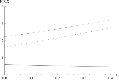
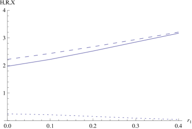
Figure 4: Plot of number entropy $H[m]$ (large-dashed line), phase knowledge $R[\theta]$ (small-dashed line) and entropy excess $X[m,\theta]$ (bold line) for an anharmonic oscillator initially in squeezed Kerr state, with respect system squeezing $r_{1}$ (39). Figure (a) represents the pure state case, while Figure (b) represents the system subjected to QND interaction with a squeezed thermal bath with temperature $T=1$ and evolution time $t=1$. The parameters used are $\omega=1$, $\omega_{c}=100$, $\gamma_{0}=0.1$, $\psi=\pi/4$, $|\alpha|^{2}=5$, $\theta_{0}=0$, $\chi=0.02$, $\lambda=0.02$, and with bath squeezing parameters $r=0.1$, $a=0$.

Using ${\cal P}(\theta)$ (42) in Eq. (9) to get the phase knowledge, $p(m)$ (43) to get the number entropy and using these in Eq. (11) we get the entropy excess which are plotted in Figures 4. In Figure 4 (a), depicting unitary evolution, it is seen that phase knowledge almost exactly compensates for the growth of ignorance of number, as a functions of $r_{1}$, whereas , in Figure 4 (b), phase knowledge is rapidly lost, depicting clearly the influence of the environment. The principle of entropy excess, Eq. (11), is clearly seen to be satisfied for unitary evolution as well as when the anharmonic system is interacting with its environment.

IV.2 Dissipative system-bath interaction

Here the system-reservoir interaction is such that $[H_{S},H_{SR}]\neq 0$ resulting in decoherence along with dissipation.

(A). System of harmonic oscillator interacting with a thermal bath resulting in a Lindblad evolution:

The initial state of the system is a superposition of coherent states which are $180^{\circ}$ out of phase with respect to each other mb92 .

$$|\psi\rangle=A^{1/2}(|\alpha\rangle+e^{i\phi}|-\alpha\rangle),$$ (44)

where $\alpha=|\alpha|e^{i\phi_{0}}$ and

$$A=\frac{1}{2}[1+\cos(\phi)e^{-2|\alpha|^{2}}]^{-1}.$$ (45)

The state $|\psi\rangle$ for $\phi=0$ would be an even coherent state and for $\phi=\pi$ would be an odd coherent state. The reduced density matrix can be shown to have the following form vb93 :

$$\rho(t)=\sum\limits_{n,m=0}^{\infty}\rho_{n,m}(t)|n\rangle\langle m|,$$ (46)

where

$$\rho_{n,m}(t) = \frac{A}{N(t)+1}\left(\frac{e^{-\gamma_{0}t/2}}{N(t)+1}\right)^{m+n}Q_{n}Q_{m}e^{i(n-m)\phi_{0}}$$ (47)

$$\times \sum\limits_{l=0}^{\infty}\left(1-\frac{e^{-\gamma_{0}t/2}}{N(t)+1}\right)^{l}\frac{|\alpha|^{2l}}{l!}\left(1+(-1)^{n+m}+(-1)^{l}[(-1)^{n}e^{i\phi}+(-1)^{m}e^{-i\phi}]\right)$$

$$\times F^{2}_{1}\left[-m,-n;l+1;4N(t)(N(t)+1)(\sinh(\gamma_{0}t/2))^{2}\right].$$

Here $F^{2}_{1}$ is the Gauss hypergeometric function ETBM , $\gamma_{0}$ is a parameter which depends upon the system-reservoir coupling strength,

$$Q_{n}=\frac{|\alpha|^{n}}{\sqrt{n!}}e^{-\frac{|\alpha|^{2}}{2}},$$ (48)

and,

$$N(t)=N_{th}(1-e^{-\gamma_{0}t}),~{}N_{th}=\left(e^{\frac{\hbar\omega}{k_{B}T}}-1\right)^{-1}.$$ (49)

The phase distribution is given by

$${\cal P}(\theta)={1\over 2\pi}\sum\limits_{m,n=0}^{\infty}\rho_{m,n}e^{i(n-m)\theta},$$ (50)

where $\rho_{m,n}$ can be obtained from Eq. (47).

The corresponding complementary number distribution is obtained, using Eq. (4), as

$$p(m)=\rho_{m,m}(t),$$ (51)

where $\rho_{m,m}$ is as in Eq. (47).

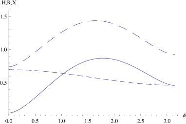
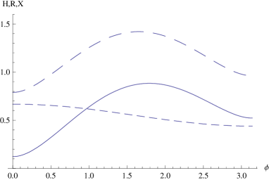
Figure 5: Plot of number entropy $H[m]$ (large-dashed line), phase knowledge $R[\theta]$ (small-dashed line) and entropy excess $X[m,\theta]$ (bold line) for a harmonic oscillator, initially in a coherent state superposition (44), as a function of the state parameter $\phi$ (44). Figure (a) pertains to the pure state case. Figure (b) represents the system subjected to a dissipative interaction with the environment for an evolution time $t=0.1$ and temperature $T=2$. The parameters used are $\omega=1$, $\gamma_{0}=0.025$, $|\alpha|^{2}=2$, $\phi_{0}$ (44) $=0$.

Using ${\cal P}(\theta)$ (50) in Eq. (9) to get the phase knowledge, $p(m)$ (51) to get the number entropy and using these in Eq. (11) we get the entropy excess which are plotted in Figures 5. From Figure 5 (a), pertaining to unitary evolution, we note that in the even cat (coherent) state ($\phi=0$), ignorance of number approximately equals phase knowledge, whereas in the odd cat (coherent) state ($\phi=\pi$) the former significantly outweighs the latter. This thus provides a complementaristic characterization of the even and odd cat states. The Figure 5 (b) shows that the effect of the dissipative environment causes phase to become randomized, leading to an increased entropy excess at all $\phi$ (44). The principle of entropy excess, Eq. (11), is clearly seen to be satisfied, for both unitary as well as dissipative evolution.

(B). System of anharmonic oscillator weakly interacting with a thermal bath:

The total Hamiltonian depicting a third-order non-linear oscillator coupled to a reservoir of oscillators jp84 , assumed to be initially in a thermal state, is

$$H=\hbar\left[\omega(a^{\dagger}a+\frac{1}{2})+\kappa a^{\dagger 2}a^{2}+\sum\limits_{j}\omega_{j}(b^{\dagger}_{j}b_{j}+\frac{1}{2})+\sum\limits_{j}(\kappa_{j}b_{j}a^{\dagger}+\kappa^{*}_{j}b^{\dagger}_{j}a)\right].$$ (52)

The reduced density matrix of the anharmonic oscillator, starting from the initial coherent state $|\xi(0)\rangle$ $=$ $||\xi(0)|e^{i\phi_{0}}\rangle$, can be solved and made use of to obtain the phase distribution

$${\cal P}(\theta) = {1\over 2\pi}\sum\limits_{m,n=0}^{\infty}\rho_{m,n}e^{i(n-m)\theta}$$ (53)

$$= \frac{1}{2}\sum\limits_{m,n=0}^{\infty}(m!n!)^{1/2}f_{n,m}(t)e^{i(n-m)\theta}.$$

Here

$$f_{m,n}(t) = \exp\left([-2i\kappa(m-n)+\frac{\gamma_{0}}{2}]t\right)\left(E_{m-n}(t)\right)^{m+n+1}\sum\limits_{l=0}^{\infty}\frac{1}{l!}\left[\frac{N_{th}+1}{N_{th}}g_{m-n}(t)\right]^{l}\frac{(m+l)!(n+l)!}{m!n!}$$ (54)

$$\times f_{m+l,n+l}(0)F^{2}_{1}\left[-m,-n;l+1;\frac{4N_{th}(N_{th}+1)}{\Delta^{2}}(\sinh(\gamma_{0}\Delta t/2))^{2}\right].$$

In the above equation, $f_{m+l,n+l}(0)$ contains information about the initial state of the system and for the initial coherent state $|\xi(0)\rangle$ $=$ $||\xi(0)|e^{i\phi_{0}}\rangle$ is given by

$$f_{m,n}(0)=\frac{1}{\pi}\frac{\xi^{m*}(0)}{m!}\frac{\xi^{n}}{n!}.$$ (55)

$F^{2}_{1}$ is the Gauss hypergeometric function ETBM , $\gamma_{0}$ is a parameter which depends upon the system-reservoir coupling strength and $N_{th}$ is as defined above. Also

$$E_{m-n}(t)=\frac{\Delta}{\Omega\sinh(\gamma_{0}\Delta t/2)+\Delta\cosh(\gamma_{0}\Delta t/2)},$$ (56)

$$g_{m-n}(t)=\frac{2N_{th}}{\Omega+\Delta\coth(\gamma_{0}\Delta t/2)},$$ (57)

$$\Omega\equiv\Omega_{m-n}=1+2N_{th}-i\frac{2\kappa}{\gamma_{0}}(m-n),$$ (58)

and

$$\Delta\equiv\Delta_{m-n}=\left[\Omega^{2}-4N_{th}(N_{th}+1)\right]^{1/2}.$$ (59)

The corresponding complementary number distribution is obtained, using Eq. (4), as

$$p(m)=\pi n!f_{m,m}(t),$$ (60)

where $f_{m,m}$ can be obtained from Eq. (54).

Figure 6: Phase distribution ${\cal P}(\theta)$ as a function of $\theta$ for the dissipative anharmonic oscillator initially in a coherent state. The bold curve represents unitary evolution while the other curves represent temperature $T=0$ and evolution times $t=1,5$ and $10$ for the dotted, large-dashed and dot-dashed curves, respectively. The parameters used are $\omega=1$, $|\xi(0)|^{2}=2$, $\phi_{0}=0$ ($|\xi(0)|$, $\phi_{0}$ are the initial state parameters), $\gamma_{0}=0.01$ and $\kappa=0.05$ (52).

Figure 7: Number entropy $H[m]$ (large-dashed line), phase knowledge $R[\theta]$ (small-dashed line) and entropy excess $X[m,\theta]$ (bold line) for an anharmonic oscillator system, initially in a coherent state, with respect to initial state parameter $|\xi_{0}|$ ($=|\xi(0)|$), subjected to a dissipative interaction where the parameters are as in the above figure. The figures depict an evolution time $t=2$ and temperature $T=0$. It can be shown that, in contrast to the corresponding harmonic oscillator case (Fig. 1(a)), increase in average number ($|\xi_{0}|$) is not accompanied by a corresponding increase in phase knowledge.

The phase distribution ${\cal P}(\theta)$ (53) is plotted in Figure 6 from which we see that with increase in time, phase gets randomized resulting in phase diffusion. Using this ${\cal P}(\theta)$ (53) in Eq. (9) to get the phase knowledge, $p(m)$ (60) to get the number entropy and using these in Eq. (11) we get the entropy excess which are plotted in Figure 7. The effect of the dissipative interaction is seen to manifest in the increased phase randomization and entropy excess with increase in the state parameter $|\xi_{0}|$. The principle of entropy excess, Eq. (11), is, again, clearly seen to be satisfied.

V Atomic System

Here we study entropy excess (11) for number-phase complementarity in (finite-level) atomic systems, briefly revisiting results obtained from the perspective of an upper bound on the knowledge-sum of complementary variables in Ref. rs07 . An interesting generalization of the knowledge-sum of complementary variables could be made, in the context of quantum communication, using the information exclusion relations developed in mh95 . As pointed out earlier, the knowledge-sum approach cannot be applied to infinite dimensional systems, whereas the principle of entropy excess can be applied to finite as well as infinite dimensional systems, making it a more flexible tool for studying number-phase complementarity in a host of systems.

As an application of the principle, it is appropriate to study the effect of noise. This we do for noise from both non-dissipative as well as dissipative interactions of the atomic system $S$ with its environment, which is modelled as a bath of harmonic oscillators starting in a squeezed thermal state bg06 ; gp ; sqgen . In Section V.2 we consider the effect of the phase damping channel, which is the information theoretic analogue of the non-dissipative open system effect bg06 ; gp , while in Section V.3 we consider the effect of the squeezed generalized amplitude damping channel which is the information theoretic analogue of the dissipative open system effect gp ; sqgen .

V.1 The principle of entropy excess in atomic systems

For a (noiseless) two-level (spin-1/2) system, the plot of entropy $H[m]$ for all atomic coherent states is given by the large-dashed curve in Figure 8(a). The equatorial states on the Bloch sphere, corresponding to $\alpha^{\prime}=\pi/2$, are the maximum knowledge state (MXK) states of $\phi$, and are precisely equivalent to the minimum knowledge state (MNK) states of $m$ (characterized by $H[m]=1$), as can be seen from comparing the large-dashed and small-dashed curves in the Figure. Thus number and phase share with MUBs the reciprocal property that maximum knowledge of one of them is simultaneous with minimal knowledge of the other, but differs from MUBs in that the maximum possible knowledge of $\phi$ is less than $\log(d)=1$ bit, essentially on account of its POVM nature.

Two variables form a quasi-MUB if any MXK state of either variable is an MNK state of the other, where the knowledge of the MXK state may be less than $\log d$ bits. Thus, $J_{z}$ and $\phi$ are quasi-MUB’s (but not MUB’s).

From the dot-dashed curve in the Figures (8), we numerically find an expression of the uncertainty principle to be

$$X[m,\phi]\equiv H[m]-R[\phi]\geq 0$$ (61)

for all pure states in ${\bf C}^{2}$, in conformity with Eq. (6) and hence also in agreement with the principle of entropy excess (11). As $\phi$ is a POVM but $m$ represents a regular Hermitian observable, in general $X[m,\phi]\neq X[\phi,m]$. The inequality is saturated only for the Wigner-Dicke states (as seen from the dot-dashed curve in the Figure), when $H[m]$ and $R[\phi]$ identically vanish.

As an expression of the uncertainty principle, the relation (61) still leaves some room for improvement. First, it is not a tight bound. In particular, for equatorial states it permits $R[\phi]$ to be as high as 1, whereas as seen from the small-dashed curve in Figure 8, the maximum value of $R[\phi]$, which is $r_{\phi}\approx 0.245$.

Following Ref. rs07 , one way to address this problem is to modify (61) to the inequality

$$X^{\mu}[m,\phi]\equiv H[m]-\mu R[\phi]\geq 0$$ (62)

for all pure states in ${\bf C}^{2}$, where parameter $\mu$ $(>0)$ is chosen to be the largest value such that inequality (62) is satified over all state space. Through a numerical search, we found that $\mu\approx 4.085$ for dimension $d=2$ and $\mu\approx 1.973$ for $d=4$. From the concavity of $H[m]$ and the convexity of $R[\phi]$, it follows that Eq. (62) holds for any mixed state. The small-dashed and dotted curves are, respectively, $R[\phi]$ and $\mu R[\phi]$. Comparing their corresponding curves in the Figure, we note the tighter bound imposed by $X_{\mu}[m,\phi]$ than $X[m,\phi]$.

V.2 Application to the phase damping channel

The ‘number’ and phase distributions for a qubit, $H_{S}=\frac{\hbar\omega}{2}\sigma_{z}$, starting from an atomic coherent state $|\alpha^{\prime},\beta^{\prime}\rangle$, and subjected to a phase damping channel due to its interaction with a squeezed thermal bath, are sb06 ; bg06

$$p(m) = \left(\begin{array}[]{c}2j\\ j+m\end{array}\right)(\sin(\alpha^{\prime}/2))^{2(j+m)}(\cos(\alpha^{\prime}/2))^{2(j-m)}$$ (65)

$${\cal P}(\phi) = {1\over 2\pi}\left[1+{\pi\over 4}\sin(\alpha^{\prime})\cos(\beta^{\prime}+\omega t-\phi)e^{-(\hbar\omega)^{2}\gamma(t)}\right].$$ (66)

Figure 8: Entropy excess of a two level system subjected to QND interaction starting in an atomic coherent state $|\alpha^{\prime},\beta^{\prime}\rangle$, as a function of $\alpha^{\prime}$, with $\beta^{\prime}=0.0$. The large-dashed (resp., small-dashed) line represents $H[m]$ (resp., $R[\phi]$). The dotted-curve represents $\mu R[\phi]$ (where $\mu=4.085$). The solid (resp., dot-dashed) curve represents the entropy excess $X_{\mu}$ (resp. $X$); (a) depicts the noiseless case . There is no $\beta$-dependence; (b) depicts the case of QND interaction. The parameters used are $\omega=1.0$, $\omega_{c}=100$, $\gamma_{0}$ (69) $=0.025$, bath squeezing parameters (73) $r=0.5$ and $a=0$. The plots in the figure (b) are for a temperature $T=10$ and an evolution time $t=1$. We note the symmetry in the figure about $\alpha^{\prime}=\pi/2$. In (a), the points where $X_{\mu}=0$, namely the polar and the equatorial states, represent the coherent state. If complementarity is expressed in terms of knowledge sum rs07 , these states correspond to maximum knowledge states.

For completeness, the function $\gamma(t)$ appearing in the above equation is given in Appendix A. We note the symmetry preserved in Figures (8) (a) and (b), about $\alpha^{\prime}=\pi/2$, the equatorial states. In the case of $R[\phi]$, this is because of symmetry of $\sin(\alpha^{\prime})$, as in Eq. (66) for ${\cal P}(\phi)$ about $\pi/2$, whereas in the case of $H[m]$, the symmetry comes about because the $\cos(\cdot)$ and $\sin(\cdot)$ functions, in Eq. (66) for $p(m)$, appear only as an even power. For QND interaction $p(m)$ is time-invariant, whereas ${\cal P}(\phi)$ evolves in a way that does not affect this symmetry.

Figure 8(b) depicts the effect of phase damping noise on the number entropy $H[m]$ (obtained by using the number distribution $p(m)$ (66)), phase knowledge $R[\phi]$ (obtained by using the phase distribution ${\cal P}(\phi)$ (66)) , $\mu R[\phi]$, $X[m,\phi]$ (by using Eq. (11)) and $X_{\mu}[m,\phi]$. Comparing it with the noiseless case, as in Figure 8(a), we find that $H[m]$ remains invariant because $p(m)$ is not affected when a system undergoes a QND interaction, but there is an increase in $X_{\mu}$ because of phase randomization with time.

V.3 Application to the squeezed generalized amplitude damping channel

The ‘number’ and phase distributions for a qubit starting from an atomic coherent state $|\alpha^{\prime},\beta^{\prime}\rangle$, and subjected to a squeezed generalized amplitude damping channel sqgen due to its interaction with a squeezed thermal bath, are sr07 ,

$$p(m=1/2,t)=\frac{1}{2}\left[\left(1-\frac{\gamma_{0}}{\gamma^{\beta}}\right)+\left(1+\frac{\gamma_{0}}{\gamma^{\beta}}\right)e^{-\gamma^{\beta}t}\right]\sin^{2}(\alpha^{\prime}/2)+\frac{\gamma_{-}}{\gamma^{\beta}}\left(1-e^{-\gamma^{\beta}t}\right)\cos^{2}(\alpha^{\prime}/2),$$ (67)

and

$${\cal P}(\phi) = \frac{1}{2\pi}\left[1+\frac{\pi}{4\alpha}\sin(\alpha^{\prime})\Big{\{}\alpha\cosh(\alpha t)\cos(\phi-\beta^{\prime})+\omega\sinh(\alpha t)\sin(\phi-\beta^{\prime})\right.$$ (68)

$$\left.-\gamma_{0}\chi\sinh(\alpha t)\cos(\Phi+\beta^{\prime}+\phi)\Big{\}}e^{-\frac{\gamma^{\beta}t}{2}}\right].$$

A derivation of Eqs. (67) and (68) can be found in Ref. sr07 . For completeness, the parameters appearing in these equations are given in Appendix B.

Figures 9(a) and (b) depict the effect of squeezed generalized amplitude damping noise on the functions depicted in the noiseless case of Figure 8(a), without and with bath squeezing, respectively. Comparing them with the noiseless case, we find as expected that noise impairs both number and phase knowledge. If the dependence on $\beta^{\prime}$ is taken into consideration (cf. Ref. sr07 ), it can be shown that squeezing has the beneficial effect of relatively improving phase knowledge for certain regimes of the parameter space, and impairing them in others. This property can be shown to improve the classical channel capacity sqgen . Further, bath squeezing can be shown to render $R[\phi]$ dependent on $\beta^{\prime}$. On the other hand, it follows from Eq. (67) that $R[m]$ is independent of $\beta^{\prime}$, so that $X[m,\phi]$ is dependent on $\beta^{\prime}$. This stands in contrast to that of the phase damping channel, where inspite of squeezing, $X[m,\phi]$ remains independent of $\beta^{\prime}$ and, furthermore, squeezing impairs knowledge of $\phi$ in all regimes of the parameter space.

Figure 9: Entropy excess of a two level system subjected to a dissipative interaction starting in an atomic coherent state $|\alpha^{\prime},\beta^{\prime}\rangle$, as a function of $\alpha^{\prime}$, with $\beta^{\prime}=0.0$. The large-dashed (resp., small-dashed) line represents $H[m]$ (resp., $R[\phi]$). The dotted-curve represents $\mu R[\phi]$. The solid (resp., dot-dashed) curve represents the entropy excess $X_{\mu}$ (resp. $X$). Here $\omega=1.0$, $\omega_{c}=100$, $\Phi$ (78)$=\pi/8$, $\gamma_{0}=0.025$, with the evolution time $t=1$ and temperature $T=10$: (a) bath squeezing parameter $r$ (78)=$0$; (b) $r=1$. Comparison of (b) with (a) shows that squeezing impairs both number and phase knowledge, leading to an increase in the entropy excess $X_{\mu}$ (and $X$).

VI Discussions and Conclusions

In this paper, we have recast the number-phase complementarity for finite dimensional atomic as well as infinite dimensional oscillator, discrete (Hermitian) as well as continuous (positive operator) valued, systems as a lower bound on an entropic measure called the entropy excess. For maximally complementary systems, the bound is 0, independent of the system dimension. This is in contrast to the conventional entropy sum principle, which has a lower bound of $\log d$. To tighten the constraint imposed by the bound on $R[\phi]$, we replace this quantity by $\mu R[\phi]$, where $\mu$ is a positive number with values (approximately) 4, 2 and 1 for two-, four- and infinite-dimensional systems. Thus dimensional dependence of the inequality enters indirectly through the form $\mu=\mu(d)$. Encouraged by the above numerical-analytical pattern, we conjecture that as the system dimension increases from two to infinity, $\mu$ falls monotonically from about 4 to 1.

In this work, we have made precise the sense in which the variables $p(m)$ and $P(\phi)$ may be thought of as or differ from conventional complementary variables as96 . There are two main differences as follows. First: whereas states of maximum number knowledge (the eigenstates of the number operator) have the maximum knowledge of $\log d$ bits, the maximum phase knowledge states have less than $\log d$ bits, phase being a POVM. This was the motivation for introducing the weight quantity $\mu$. Second: even more remarkably, states of maximum phase knowledge do not correspond to equal amplitude superpositions of number states. In other words, the unbiasedness is not mutual, but one-way, a situation we characterize as one-way unbiased bases rs07 .

In the second aspect of our work, the above analysis is applied to physically relevant initial conditions of the system for unitary as well as non-unitary evolution, due to the interaction of the system with its environment. The system-reservoir interactions are chosen such that both dephasing (decoherence without dissipation) as well as dissipative (decoherence with dissipation) effects on the system evolution are studied.

Some interesting features seen were, for e.g., a harmonic oscillator starting out from an initial superposition of coherent (cat) states. The entropy excess principle was seen to provide an interesting complementaristic characterization of the even and the odd cat states, in that the excess is almost zero for the even state, indicating that ignorance of number approximately equals phase knowledge while in the odd state, the entropy excess is finite indicating that there the ignorance of number significantly outweighs knowledge of phase.

Our entropy-based formalism can modify current approaches to number-phase complementarity: e.g., one can study complementarity in conjunction with such phenomena as nonlinearity induced coherences and atomic squeezing in an effectively finite-level atomic system. In the conventional approach, complementarity can be graphically demonstrated by the constrasting behavior of the number and phase distributions (eg., Figs 1 and 2 of Ref. as96 ).

As a concrete application to a finite dimensional system in an experimental scenario, we consider the energy manifold of the four levels of (for instance) ${}^{85}Rb$ atom. This is first mapped to a pseudo-spin system of spin 3/2 while the effect of selection rules of atomic transitions in ${}^{85}Rb$ is preserved arch . Complementarity can then be studied using (entropic) knowledge of the number and phase variables as a function of laser detuning and vis-à-vis atomic phenomena like coherent population trapping (CPT) or electromagnetically induced transparency (EIT). For example, simulations indicate an increase in phase knowledge accompanying the formation of the CPT state. Noting that $\langle\theta,\phi|J_{-}|\theta,\phi\rangle=j\sin\theta e^{i\phi}$, where $J_{-}\equiv J_{x}-J_{y}$, one can detect $\phi$ in a practical, interferometric set-up by applying $J_{-}$ to one of the two interferometric arms implemented in an atom-laser system. With appropriate adjustments, $\phi$ will then manifest as a phase shift in the interference pattern.

Appendix A Some expressions pertaining to the phase damping channel

For the case of an Ohmic bath with spectral density

$$I(\omega)={\gamma_{0}\over\pi}\omega e^{-\omega/\omega_{c}},$$ (69)

where $\gamma_{0}$ and $\omega_{c}$ are two bath parameters characterizing the quantum noise, it can shown that using Eq. (69) one can obtain bg06

$$\eta(t)=-{\gamma_{0}\over\pi}\tan^{-1}(\omega_{c}t),$$ (70)

and

$$\gamma(t)={\gamma_{0}\over 2\pi}\cosh(2r)\ln(1+\omega^{2}_{c}t^{2})-{\gamma_{0}\over 4\pi}\sinh(2r)\ln\left[{\left(1+4\omega^{2}_{c}(t-a)^{2}\right)\over\left(1+\omega^{2}_{c}(t-2a)^{2}\right)^{2}}\right]-{\gamma_{0}\over 4\pi}\sinh(2r)\ln(1+4a^{2}\omega^{2}_{c}),$$ (71)

in the $T=0$ limit, where the resulting integrals are defined only for $t>2a$. In the high $T$ limit, $\gamma(t)$ can be shown to be sb06

$$\gamma(t) = {\gamma_{0}k_{B}T\over\pi\hbar\omega_{c}}\cosh(2r)\left[2\omega_{c}t\tan^{-1}(\omega_{c}t)+\ln\left({1\over 1+\omega^{2}_{c}t^{2}}\right)\right]-{\gamma_{0}k_{B}T\over 2\pi\hbar\omega_{c}}\sinh(2r)\Bigg{[}4\omega_{c}(t-a)\tan^{-1}\left(2\omega_{c}(t-a)\right)$$ (72)

$$- 4\omega_{c}(t-2a)\tan^{-1}\left(\omega_{c}(t-2a)\right)+4a\omega_{c}\tan^{-1}\left(2a\omega_{c}\right)+\ln\left({\left[1+\omega^{2}_{c}(t-2a)^{2}\right]^{2}\over\left[1+4\omega^{2}_{c}(t-a)^{2}\right]}\right)+\ln\left({1\over 1+4a^{2}\omega^{2}_{c}}\right)\Bigg{]},$$

where, again, the resulting integrals are defined for $t>2a$. Here we have for simplicity taken the squeezed bath parameters as

$$\cosh\left(2r(\omega)\right) = \cosh(2r),~{}~{}\sinh\left(2r(\omega)\right)=\sinh(2r),$$

$$\Phi(\omega) = a\omega,$$ (73)

where $a$ is a constant depending upon the squeezed bath. The results pertaining to a thermal bath can be obtained from the above equations by setting the squeezing parameters $r$ and $\Phi$ to zero.

Appendix B Some expressions pertaining to the squeezed generalized amplitude damping channel

Here the reduced dynamics of the two level atomic system interacting with a squeezed thermal bath under a weak Born-Markov and rotating wave approximation is studied. This implies that here the system interacts with its environment via a non-QND interaction, i.e., $[H_{S},H_{SR}]\neq 0$ such that along with a loss in phase information, energy dissipation also takes place.

The parameter $\alpha$ (Eq. (68)) is given by

$$\alpha=\sqrt{\gamma^{2}_{0}|M|^{2}-\omega^{2}}.$$ (74)

Further

$$\gamma^{\beta}=\gamma_{0}(2N+1),$$ (75)

and

$$\gamma_{-}=\gamma_{0}N,$$ (76)

where

$$N=N_{\rm th}(\cosh^{2}(r)+\sinh^{2}(r))+\sinh^{2}(r),$$ (77)

$$M=-\frac{1}{2}\sinh(2r)e^{i\Phi}(2N_{\rm th}+1)\equiv\chi e^{i\Phi},$$ (78)

and

$$N_{\rm th}={1\over e^{{\hbar\omega\over k_{B}T}}-1}.$$ (79)

Here $N_{\rm th}$ is the Planck distribution giving the number of thermal photons at the frequency $\omega$ and $r$, $\Phi$ are squeezing parameters. The analogous case of a thermal bath without squeezing can be obtained from the above expressions by setting these squeezing parameters to zero. $\gamma_{0}$ is a constant typically denoting the system-environment coupling strength.

References

- (1) H. Maassen and J. B. M. Uffink, Phys. Rev. Lett. 60, 1103 (1988).
- (2) M. Nielsen and I. Chuang, Quantum Computation and Quantum Information (Cambridge 2000).
- (3) A. Galindo, M.A. Martin-Delgado, Rev. Mod. Phys. 74, 347 (2000).
- (4) M. Ohya and D. Petz, Quantum Entropy and Its Use (Springer-Verlag, New York, 1993).
- (5) K. Kraus, Phys. Rev. D 35, 3070 (1987).
- (6) D. Deutsch, Phys. Rev. Lett. 50, 631 (1983).
- (7) H. Partovi, Phys. Rev. Lett. 50, 1883 (1983).
- (8) D. T. Pegg and S. M. Barnett, J. Mod. Opt. 36, 7 (1989); Phys. Rev. A 39, 1665 (1989).
- (9) I. D. Ivanovic, J. Phys. A 14, 3241 (1981).
- (10) T. Durt, J. Phys. A: Math. Gen. 38, 5267 (2005).
- (11) S. Abe, Phys. Lett. A 166, 163 (1992).
- (12) S. Wehner and A. Winter, eprint arXiv:0710.1185.
- (13) D. Petz, Reports on Mathematical Physics: 59, 209 (2007).
- (14) R. Srikanth and S. Banerjee, Euro Phys. J. D. 53, 217 (2009); eprint arXiv:0711.0875.
- (15) S. Kullback and R. A. Leibler, Ann. of Math. Stat. 22, 79 (1951).
- (16) P. Hayden, R. Jozsa, D. Petz and A. Winter, eprint arXiv:quant-ph/0304007.
- (17) W. H. Louisell, Quantum Statistical Properties of Radiation (John Wiley and Sons, 1973).
- (18) S. Banerjee and R. Ghosh, J. Phys. A: Math. Theo. 40, 13735 (2007); eprint quant-ph/0703054.
- (19) V. Perinova, A. Luks and J. Perina, Phase in Optics (World Scientific, Singapore, 1998).
- (20) P. A. M. Dirac, Proc. R. Soc. Lond. A 114, 243 (1927).
- (21) L. Susskind and J. Glogower, Physics 1, 49 (1964).
- (22) P. Carruthers and M. M. Nieto, Rev. Mod. Phys. 40, 411 (1968).
- (23) J. H. Shapiro, S. R. Shepard and N. C. Wong, Phys. Rev. Lett. 62, 2377 (1989).
- (24) W. P. Schleich and S. M. Barnett (eds.), Quantum Phase and Phase Dependent Measurements, Physica Scripta Special issue T48 (1993).
- (25) J. H. Shapiro and S. R. Shepard, Phys. Rev. A 43, 3795 (1991).
- (26) M. J. W. Hall, Quantum Opt. 3, 7 (1991).
- (27) G. S. Agarwal, S. Chaturvedi, K. Tara and V. Srinivasan, Phys. Rev. A 45, 4904 (1992).
- (28) S. Banerjee, J. Ghosh and R. Ghosh, Phys. Rev. A 75, 062106 (2007).
- (29) S. Banerjee and R. Srikanth, Phys. Rev. A 76, 062109 (2007).
- (30) G. S. Agarwal and R. P. Singh, Phys. Lett. A 217, 215 (1996).
- (31) M. A. Rashid, J. Math. Phys. 19, 1391 (1978).
- (32) G. S. Agarwal and R. R. Puri, Phys. Rev. A 41, 3782 (1990).
- (33) F. T. Arecchi, E. Courtens, R. Gilmore and H. Thomas, Phys. Rev. A 6, 2211 (1972).
- (34) R. H. Dicke, Phys. Rev. 93, 99 (1954).
- (35) J. M. Radcliffe, J. Phys. A: Gen. Phys. 4, 313 (1971).
- (36) S. Massar, eprint quant-ph/0703036.
- (37) A. S. Holevo, Probabilistic and Statistical Aspects of Quantum Theory (North Holland 1982).
- (38) I. Bialynicki-Birula and J. Mycielski, Comm. Math. Phys. 44, 129 (1975).
- (39) W. Beckner, Ann. Math. 102, 159–182 (1975).
- (40) M. J. W. Hall, Journal of Modern Optics 40, 809 (1993).
- (41) M. J. W. Hall, Phys. Rev. Lett. 74, 3307 (1995); Phys. Rev. A 55, 100 (1997).
- (42) C. M. Caves and B. L. Schumaker, Phys. Rev. A 31, 3068 (1985); B. L. Schumaker and C. M. Caves, Phys. Rev. A 31, 3093 (1985).
- (43) M. O. Scully and M. S. Zubairy, Quantum Optics (Cambridge University Press, Cambridge, 1997).
- (44) C. C. Gerry and R. Grobe, Phys. Rev. A 49, 2033 (1994).
- (45) M. V. Satyanarayana, Phys. Rev. D 32, 400 (1985); P. Marian, Phys. Rev. A 44, 3325 (1991).
- (46) A. Erdelyi, W. Magnus, F. Oberhettinger and F. G. Tricomi, Higher Transcendental Functions, Vol. I (McGraw-Hill, New York, 1953).
- (47) M. Brune,S. Haroche, J. M. Raimond, L. Davidovich and N. Zagury, Phys. Rev. A 45, 5193 (1992).
- (48) V. Buzek, Ts. Gantsog and M. S. Kim, Physica Scripta Special issue T48, 131 (1993).
- (49) J. Perina, Quantum Statistics of Linear and Nonlinear Optical Phenomena (Reide, Dordrecht, 1984).
- (50) S. Banerjee and R. Srikanth, Euro. Phys. Jr. D 46, 335 (2008); eprint quant-ph/0611161.
- (51) R. Srikanth and S. Banerjee, Phys. Rev. A 77, 012318 (2007); arXiv:0707.0059.
- (52) A. Sharma, R. Srikanth, S. Banerjee and H. Ramachandran, in preparation.