Universal protection of unitary evolution from slow noise: dynamical control pushed to the extreme

Abstract

We propose a technique that allows to simultaneously perform universal control of the evolution operator and compensate for the first order contribution of an arbitrary Hermitian constant noise. We show that, at least, a three-valued Hamiltonian is needed in order to protect the system against any such noise. This technique is illystrated by an explicit algorithm for a control sequence that is applied to numerically design a safe two-qubit gate.

I Introduction

Within the last decades, quantum control has emerged as one the most fruitful fields in both theoretical and experimental physics BS90 ; DA08 . In particular, it is of crucial importance in quantum computation NC00 . To process the information stored in the computer state, one must indeed be able to generate any prescribed unitary evolution operator on the computer — or, at least a universal set of such operators, unaffected by quantum errors arising from the interaction with the environment.

Different strategies have been developed to control the evolution of closed quantum systems, including optimal control approaches PDR88 ; PK02 ; SGL99 ; OKF98 ; SR90 and algebraic methods RFRO00 ; RSDRP95 ; SGRR02 ; ZR99 . To deal with open quantum systems, schemes have been designed to correct/avoid the undesired effects due to the environment. Quantum error-correcting codes (QEC) S95 ; NC00 ; KL97 ; G96 ; CS96 and approaches based on the quantum Zeno effect BAC05 ; BHK04 use redundancy of encoding as a way to recover information after the errors occur. Topological protection IFIITB02 takes advantage of the symmetries of the system to safely store information in so-called Decoherence Free Subspaces LBKW01 ; LBKW01b ; KBLW01 . An alternative to QEC that is substantially less resource-intensive is dynamical decoupling (DD) VZKTDD ; KL05 ; Uhrig07 . In DD one applies a succession of short and strong pulses to the system, designed to stroboscopically decouple it from the environment. Similar in spirit to DD, but more general, is the method we term here “dynamical control by modulation” (DCM), wherein one may apply to the system a sequence of arbitrarily-shaped pulses whose duration may vary anywhere from the stroboscopic limit to that of continuous dynamical modulation BAC05 ; KK05 ; Agarwal99 ; Alicki04 ; Facchi05 ; GKK06 . In the DCM approach, the decoherence rate is governed by a universal expression, in the form of an overlap between the bath-response and modulation spectra. In such methods, it is however not clear a priori whether one can, at the same time, protect the system from noise and perform universal control of its evolution operator.

In this paper we investigate this question by asking whether it is possible to perform any arbitrarily chosen evolution of a quantum system while compensating for all Hermitian static noises. To be more specific, our goal here is to show how to design a time-dependent control Hamiltonian which can, at the same time, impose a chosen evolution to the system and eliminate the first order action of any Hermitian static noise. We show that, contrary to strict evolution control problems, this objective cannot be achieved with only two-valued Hamiltonians but requires the use of at least three control operators. We go on to show that even a null third operator, causing the system to evolve under the action of noise only, is enough. Inspired by a previous result HA99 , we propose a new algorithm able to compute the appropriate control sequence for any given desired evolution. As an application, this algorithm was run to design a safe $CNOT$ gate.

The paper is structured as follows. We first set the problem to solve and give the explicit conditions the evolution matrix must fulfill. Then we show that these conditions are impossible to meet by a two-valued control Hamiltonian. Slightly modifying the two-stage procedure by allowing for extra steps during which the control Hamiltonian is set to zero, we describe an algorithm able to compute an appropriate protected control sequence. An application to a two-qubit gate is finally proposed.

II Conditions for first-order noise elimination

Let us consider an $N$-level quantum system whose Hamiltonian consists of a controllable part, denoted by $H_{c}\left(t\right)$, and an unknown but static noise contribution, which can be written as a linear combination $\mathcal{N}=\sum_{i}\hbar\varepsilon_{i}G_{i}$ of the Hermitian traceless generators $\left\{G_{i},i=1,\ldots,N^{2}-1\right\}$ of $su(N)$. The evolution matrix satisfies the dynamical equation

$$\imath\hbar\frac{\partial U\left(t\right)}{\partial t} = \left(H_{c}\left(t\right)+\mathcal{N}\right)U\left(t\right)$$ (1)

$$U\left(0\right) = I.$$ (2)

Upon transforming to the interaction picture relative to $H_{c}$, one isolates the evolution $\widetilde{U}\left(t\right)$ due to the noise only: defining

$$U_{c}\left(t\right)\equiv T\exp\left\{\frac{1}{\imath\hbar}\int_{0}^{t}H_{c}\left(s\right)ds\right\}$$ (3)

the evolution induced by the control Hamiltonian alone, where $T$ denotes the chronological product, one sets $\widetilde{U}\left(t\right)\equiv U_{c}^{\dagger}\left(t\right)U\left(t\right)$, which satisfies

$$\imath\hbar\frac{\partial\widetilde{U}}{\partial t} = \left[U_{c}^{\dagger}\left(t\right)\mathcal{N}U_{c}\left(t\right)\right]\widetilde{U}\left(t\right)$$ (4)

$$= \left[\sum_{i}\hbar\varepsilon_{i}U_{c}^{\dagger}\left(t\right)G_{i}U_{c}\left(t\right)\right]\widetilde{U}\left(t\right)$$ (5)

$$\widetilde{U}\left(0\right) = I.$$ (6)

The first order contribution of the noise to the evolution is thus given by the second term in the Dyson expansion of $\widetilde{U}\left(t\right)$ for the accumulated action, that is

$$\widetilde{U}^{\left(1\right)}\left(t\right)=\sum_{i}\varepsilon_{i}\int_{0}^{t}U_{c}^{\dagger}\left(s\right)G_{i}U_{c}\left(s\right)ds.$$ (7)

Our goal is to design a control Hamiltonian $H_{c}\left(t\right)$, such that, at the end of the control sequence, say at time $T_{c}$, the evolution operator takes an arbitrarily prescribed value $U_{d}\in SU\left(N\right)$ while the first order contribution of any constant noise vanishes. We thus require

$$U_{c}\left(T_{c}\right) = U_{d}$$ (8)

and, for any set of constants $\left\{\varepsilon_{i}\right\}$,

$$\widetilde{U}^{\left(1\right)}\left(T_{c}\right)=\sum_{i}\varepsilon_{i}\int_{0}^{T_{c}}U_{c}^{\dagger}\left(s\right)G_{i}U_{c}\left(s\right)ds=0,$$ (9)

that is

$$\forall i,\quad\int_{0}^{T_{c}}U_{c}^{\dagger}(s)G_{i}U_{c}(s)ds=0.$$ (10)

III Alternating two-valued operator sequence

Let us now focus on the two-valued alternating perturbation approach. Namely, the control Hamiltonian $H_{c}\left(t\right)$ alternates between two values $A$ and $B$ for adjustable timings which play the role of control parameters. Formally, $H_{c}\left(t\right)$ then assumes the bilinear form $H_{c}\left(t\right)=\hbar\alpha\left(t\right)A+\hbar\beta\left(t\right)B$, where $\alpha\left(t\right)$ and $\beta\left(t\right)$ are two piecewise constant functions taking the values $0,1$ and adding up to $1$. In the sudden approximation, the overall evolution operator induced by such a $K$-step control sequence has the pulsed form

$$U_{c}\left(T_{c}\right)=e^{-\imath T_{K}H_{K}}\times\ldots\times e^{-\imath T_{2}H_{2}}\times e^{-\imath T_{1}H_{1}},$$ (11)

where $H_{k}\equiv A$ when $k$ is even, $B$ when $k$ is odd, and $\sum_{k=1}^{K}T_{k}=T_{c}$.

Provided that $A$, $B$ together with their all-order commutators span $su(N)$ (the bracket generation condition), it can be shown HA99 that it is possible to design $K\propto N^{2}$ such control timings $\left\{T_{1},\ldots,T_{K}\right\}$ for which eq.(8) is met, i.e. such that

$$e^{-\imath T_{K}H_{K}}\times\ldots\times e^{-\imath T_{2}A}\times e^{-\imath T_{1}B}=U_{d}.$$ (12)

It turns out, however, that, except for the particular case $U_{d}=I$, eq.(10) cannot be satisfied for all noises. As we shall now show, there indeed always exists a $D$-dimensional uncorrectable subspace $\left(1\leq D\leq N-1\right)$ spanned by the noise operators $C_{n\in N}\equiv\frac{1}{2}\left[A+B,\left(B-A\right)^{n}\right]$. To prove this, let us first introduce the operators

$$U_{0}\equiv I,\quad U_{K\geq i\geq 1}\equiv e^{-\imath T_{i}H_{i}}\times\ldots\times e^{-\imath T_{2}A}\times e^{-\imath T_{1}B}$$ (13)

which allow us to write

$$U_{c}\left(t\right) = e^{-\imath\left(t-\sum_{k=1}^{i}T_{k}\right)H_{i+1}}U_{i}$$ (15)

$$(\text{for }{\textstyle\sum_{1}^{i}T_{k}\leq t<\sum_{1}^{i+1}T_{k}}).$$

Let us further define the superoperators $\hat{\mathcal{H}}_{i}$, whose action is given, on any operator $X$, by $\hat{\mathcal{H}}_{i}X\equiv\left[H_{i},X\right]$. We can thus write $e^{+\varepsilon H_{i}}Xe^{-\varepsilon H_{i}}=\sum_{k=0}^{\infty}\frac{\varepsilon^{k}}{k!}\hat{\mathcal{H}}_{i}^{k}X$. Since $\left[A,(B-A)^{n}\right]=\left[B,(B-A)^{n}\right]=\left[H_{i},(B-A)^{n}\right]$ for every $i$, we can set $C_{n}=\hat{\mathcal{H}}_{i}(B-A)^{n}$.

Let us now evaluate the first order effect of $C_{n}$ according to eq.(10):

$$\int_{0}^{T_{c}} U_{c}^{\dagger}(s)C_{n}U_{c}(s)ds$$ (16)

$$= \sum_{i}\int_{0}^{T_{i}}dsU_{i}^{\dagger}e^{\imath sH_{i}}\hat{\mathcal{H}}_{i}(B-A)^{n}e^{-\imath sH_{i}}U_{i}$$ (17)

$$= \sum_{i}U_{i}^{\dagger}\int_{0}^{T_{i}}ds\sum_{k=0}^{\infty}\frac{(-\imath s)^{k}}{k!}\hat{\mathcal{H}}_{i}^{k+1}(B-A)^{n}U_{i}$$ (18)

$$= \imath\sum_{i}U_{i}^{\dagger}\left[e^{\imath T_{i}H_{i}}(B-A)^{n}e^{-\imath T_{i}H_{i}}-(B-A)^{n}\right]U_{i}$$ (19)

$$= \imath\sum_{i}U_{i+1}^{\dagger}(B-A)^{n}U_{i+1}-\imath\sum_{i}U_{i}^{\dagger}(B-A)^{n}U_{i}$$ (20)

$$= \imath U^{\dagger}(T_{c})(B-A)^{n}U(T_{c})-\imath(B-A)^{n}.$$ (21)

The first order contribution we have just obtained does not depend on the specific timing parameters $T_{i}$’s but only on the final operation $U(T_{c})$; it is moreover nonzero for any $U_{d}\neq I$. Finally, according to the Cayley-Hamilton theorem, the matrix $(B-A)$ cancels its characteristic polynomial, which implies that $1\leq\dim\left[\mathrm{Span}\left(\left\{(B-A)^{n},n\in N\right\}\right)\right]\leq N-1$. As a consequence the dimension $D\equiv\dim\left[\mathrm{Span}\left(\left\{C_{n},n\in N\right\}\right)\right]$ of the uncorrectable subspace satisfies $1\leq D\leq N-1$.

Let us now examine how the two-operator Hamiltonian scheme can be modified so that both conditions eq.(8,10) are met. Suppose we have a sequence of timings $\{t_{1},\dots,t_{K}\}$. Now $U_{0}$ and $U_{n\geq 1}$ are the evolution operator at the end of the $n^{th}$ step of the control sequence as defined in eq.(13), while $U_{c}(t)$ is the evolution operator at time $t$ as defined in eq.(15). Following the method described in HA99 , the last $N^{2}-1$ timings $\{t_{K-N^{2}+2},\dots,T_{K}\}$ can be chosen such that they achieve the evolution $U_{d}\cdot U_{K-N^{2}+1}^{\dagger}$, thus satisfying the condition of eq.(8). The first order contribution of any noise $G_{i}$ can be explicitly expressed by the accumulated action

$$\mathcal{G}_{i}\equiv\sum_{n=1}^{K}U_{n}^{\dagger}g_{i,n}U_{n},$$ (22)

where $g_{i,n}\equiv\int_{0}^{T_{n}}e^{-\imath sH_{n}}G_{i}e^{+\imath sH_{n}}ds$.

Let us, at each commutation between A and B, allow for the waiting time $\tau_{l=1,\dots,K}$ during which no perturbation is applied. This amounts to adding a third value $C=0$ to the control Hamiltonian $H_{c}(t)$. We see that the overall evolution operator remains unchanged, while the first order contribution of any noise $G_{i}$ is added the term $\sum_{n=1}^{K}\tau_{n}U_{n}^{\dagger}G_{i}U_{n}$, which is a linear function of the waiting times.

Let us choose the timings $\{t_{1},\dots,t_{K-N^{2}+1}\}$ such that the coefficients of the waiting times span the entire $N^{2}\cdot(N^{2}-1)$ space. Generally this can be achieved by randomly choosing the timings. Thus, by solving a simple set of $N^{2}\cdot(N^{2}-1)$ linear equations of the form $\mathcal{G}_{i}+\sum_{n=1}^{K}\tau_{n}\mathcal{F}_{i,n}=0$ ($\mathcal{F}_{i,n}\equiv U_{n}^{\dagger}G_{i}U_{n}$) to find the waiting times $\tau_{1},\dots,\tau_{K}$, one can eliminate the first order contribution of all the noises $G_{i}$ added during the $A$, $B$ control sequences. In practice, since the waiting times $\tau_{i}$ must be positive, this requires a slightly larger $K$ and the use of linear programming methods or other minimization techniques.

IV Algorithm for a four-state system

This algorithm was applied to a model four-state system, represented in Fig. 1, which can be used to store and process two qubits of information. The four states correspond to two different angular momenta $l=0,1$: $\left|0\right\rangle\equiv\left|l=0,m_{l}=0\right\rangle$, $\left|1\right\rangle\equiv\left|l=1,m_{l}=-1\right\rangle$, $\left|2\right\rangle\equiv\left|l=1,m_{l}=0\right\rangle$ and $\left|3\right\rangle\equiv\left|l=1,m_{l}=1\right\rangle$.

This system is subject to a resonant electric and a static magnetic fields: the $\pi$-component of the electric field couples $\left|0\right\rangle$ to $\left|2\right\rangle$ while the $\sigma_{+,-}$-components couple $\left|0\right\rangle$ to $\left|1\right\rangle$, and $\left|0\right\rangle$ to $\left|3\right\rangle$, respectively; the $x,y$-component of the magnetic field couples $\left|1\right\rangle$ to $\left|2\right\rangle$ and $\left|2\right\rangle$ to $\left|3\right\rangle$ while its $z$-component shifts $\left|1\right\rangle$ and $\left|3\right\rangle$ out of resonance. Finally, in the rotating wave approximation (RWA), the total Hamiltonian of the system assumes the form

$$H_{c}= e_{-}\sigma_{-}+e_{0}\sigma_{0}+e_{+}\sigma_{+}+b_{\perp}\Lambda_{\perp}+b_{z}\Lambda_{z}$$ (23)

$$\sigma_{-}\equiv \left|1\right\rangle\left\langle 0\right|+\left|0\right\rangle\left\langle 1\right|$$ (24)

$$\sigma_{0}\equiv \left|2\right\rangle\left\langle 0\right|+\left|0\right\rangle\left\langle 2\right|$$ (25)

$$\sigma_{+}\equiv \left|3\right\rangle\left\langle 0\right|+\left|0\right\rangle\left\langle 3\right|$$ (26)

$$\Lambda_{\perp}\equiv \left|1\right\rangle\left\langle 2\right|+\left|2\right\rangle\left\langle 3\right|+\left|2\right\rangle\left\langle 1\right|+\left|3\right\rangle\left\langle 2\right|$$ (27)

$$\Lambda_{z}\equiv \left|3\right\rangle\left\langle 3\right|-\left|1\right\rangle\left\langle 1\right|$$ (28)

where $e_{-,0,+}$ and $b_{\perp,z}$ are five independent parameters, proportional to the electric and magnetic field amplitudes, respectively. By choosing two different sets $\left\{e_{-,0,+}^{A},b_{\perp,z}^{A}\right\}$ and $\left\{e_{-,0,+}^{B},b_{\perp,z}^{B}\right\}$ of such parameters, we can define two values for the Hamiltonian $H_{c}=A,B$ which may be used as our alternating perturbations.

After verifying that $A$ and $B$ satisfy the bracket generation condition, we first calculate the $K=N^{2}=16$ timings $\left\{t_{k=1,\ldots,K}^{\left(0\right)}\right\}$ which realize the identity matrix, by the method described in HA99 , based on statistical properties of the roots of the identity. By the Newton iterative method, we then compute the $K=16$ timings $\left\{t_{k=1,\ldots,K}\right\}$ which perform the transformation $CNOT^{\frac{1}{N^{2}-1}}=CNOT^{\frac{1}{15}}$, where $CNOT\equiv\left(\begin{array}[]{cccc}1&0&0&0\\ 0&1&0&0\\ 0&0&0&1\\ 0&0&1&0\end{array}\right)$.

Finally, we look for the $K\left(N^{2}-1\right)=240$ waiting times $\tau_{l=1,\ldots,K\left(N^{2}-1\right)}$ which minimize all $15$ possible noise operators to zero. By applying the complete $480$-step control sequence, consisting of the $\left(N^{2}-1\right)=15$ repetitions of the sequence $\left\{t_{k=1,\ldots,K=16}\right\}$ plus the $K\left(N^{2}-1\right)=240$ waiting periods $\left\{\tau_{l}\right\}$ with zero control after each step, we can thus impose a safe $CNOT$ gate on the system in the presence of any noise that varies slower than the control sequence.

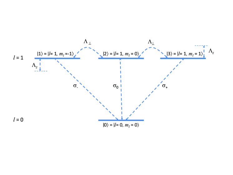
Figure 1: The two-level atomic system ($l=0,1$). The arrows show the different couplings due to the resonant electric field (operators $\sigma_{-,0,+}$) and the static magnetic field (operators $\Lambda_{\perp,z}$).

V Discussion

It is plausible that the conditions eq.(8,10) can be satisfied by an arbitrary three-valued Hamiltonian, with $C\neq 0$. We have looked for an appropriate sequence of timings with such a Hamiltonian by direct optimization of a cycle of $KN^{2}$ operations and found satisfactory numerical solutions up to $N=16$. This approach is however slower than the scheme described above.

There are several open issues regarding the universal control method proposed here. First, it is important to treat higher orders in the perturbation expansion of the noise and, in particular, explore the feasibility of a control Hamiltonian canceling the second order contribution of the noise, $i.e.$ the integrals

$$\int_{0}^{T_{c}}dt\int_{0}^{t}dsU_{c}^{\dagger}(t)G_{m}U_{c}(t)U_{c}^{\dagger}(s)G_{n}U_{c}(s)$$ (29)

for any $\left(m,n\right)$. Second, the issue of time-dependent noises is important. The present method holds for noise that slowly varies with time, compared to the control sequence. The approach must change altogether if fast noises affect the system. Finally, it is imperative to establish whether redundancy can be combined with dynamic control techniques to safely process the information, as, for example, in an ensemble of identical systems.

To conclude, we have raised the question whether universal control of evolution may be performed while compensating for the first order contribution of arbitrary constant Hermitian noise, by means of an alternating perturbation procedure. We have demonstrated that this can not be achieved by a two-valued control Hamiltonian: in that case there always exists a subspace of uncorrectable noises. If, however, we allow for waiting times, during which the system is only subject to noise, our objective becomes feasible. This has been demonstrated by an explicit algorithm that yields the appropriate control sequence, as tested on the case $N=4$. The total waiting time is of the order of half the control period. More generally, we numerically checked that a three-valued Hamiltonian can control the evolution operator and protect it against any static Hermitian noise.

G.K. acknowledges the support of the EC (SCALA and MIDAS), GIF and ISF.

References

- (1) Butkovskiy A. G. and Yu. I. Samoilenko, Control of Quantum-Mechanical Processes and Systems, Kluwer Academic Publishers, Dordrecht (Netherlands), 1990.
- (2) D’Alessandro D., Introduction to Quantum Control and Dynamics, Chapman & Hall/CRC, 2008.
- (3) Nielsen M. A. and Chuang I. L., Quantum Computation and Quantum Infomation, Cambridge University Press, Cambridge, 2000.
- (4) Peirce A. P. , Dahleh M. A. and Rabitz H., Phys. Rev. A 37 4959 (1988).
- (5) Palao J. and Kosloff R., Phys. Rev. Lett. 89 188301 (2002) .
- (6) Schirmer S. G., Girardeau M. D., Leahy J. V., Phys. Rev. A 61 012101 (1999).
- (7) Ohtsuki Y., Kono H. and Fujimura Y., J. Chem. Phys. 109 9318 (1998).
- (8) Shi S. and Rabitz H., J. Chem. Phys. 92 364 (1990).
- (9) Ramakrishna V., Flores K. L., Rabitz H. and Ober R. J., Phys. Rev. A 62 053409 (2000).
- (10) Ramakrishna V., Salapaka M. V., Dahleh M., Rabitz H. and Peirce A., Phys. Rev. A 51 960 (1995).
- (11) Schirmer S. G., Greentree A. D., Ramakrishna V. and Rabitz H., J. Phys. A: Math. Gen. 35 8315 (2002).
- (12) Zanardi P. and Rasetti M., Physics Letters A 264 94 (1999).
- (13) Shor P. W., Phys. Rev. A 52 R2493 (1995).
- (14) Knill E. and Laflamme R., Phys. Rev. A 55 900 (1997.
- (15) Gottesman D., Phys. Rev. A 54 1862 (1996).
- (16) Calderbank A. R. and Shor P. W., Phys. Rev. A 54 1098 (1996).
- (17) Brion E., Harel G., Kebaili N., Akulin V. M. and Dumer I., Europhys. Lett. 66 157 (2004).
- (18) Brion E., Akulin V. M., Comparat D., Dumer I., Harel G., Kébaili N., Kurizki G., Mazets I., and Pillet P., Phys. Rev. A 71 052311 (2005).
- (19) Ioffe L. B., Feigelman M. V., Ioselevich A., Ivanov D., Troyer M. and Blatter G., Nature 415 503 (2002).
- (20) Lidar D. A., Bacon D., Kempe J., and Whaley K. B., Phys. Rev. A 63 022306 (2001).
- (21) Lidar D. A., Bacon D., Kempe J., and Whaley K. B., Phys. Rev. A 63 022307 (2001).
- (22) Kempe J., Bacon D., Lidar D. A., and Whaley K. B., Phys. Rev. A 63 042307 (2001).
- (23) Viola L. and LloydS., Phys. Rev. A 58 2733 (1998); Zanardi P., Phys. Lett. A 258 77 (1999); Viola L., Knill E., and Lloyd S., Phys. Rev. Lett. 82 2417 (1999); Vitali D. and Tombesy D., Phys. Rev. A 59 4178 (1999); Vitali D. and Tombesy D., Phys. Rev. A 65 012305 (2001).
- (24) Khodjasteh K. and Lidar D. A., Phys. Rev. Lett. 95 180501 (2005).
- (25) Uhrig G. S., Phys. Rev. Lett. 98 100504 (2007).
- (26) Kofman A. G. and Kurizki G., Phys. Rev. Lett. 87 270405 (2001); Kofman A. G. and Kurizki G., Phys. Rev. Lett. 93 130406 (2004); Kofman A. G. and Kurizki G., IEEE Trans. Nanotechnology 4 116 (2005) .
- (27) Agarwal G. S., Phys. Rev. A 61 013809 (1999).
- (28) Alicki R. et al., Phys. Rev. A 70 010501 (2004).
- (29) Facchi P. et al., Phys. Rev. A 71 022302 (2005) .
- (30) Gordon G., Kurizki G. and Kofman A. G., Opt. Comm. 264 398 (2006) ; Gordon G. and Kurizki G., Phys. Rev. A 76 042310 (2007) ; Gordon G., Erez N and Kurizki G., J. Phys. B 40 S75 (2007)
- (31) Harel G. and Akulin V.M., Phys. Rev. Lett. 82 1, 1999.